Blade root moment sensor failure detection based on multibeam LIDAR for fault-tolerant individual pitch control of wind turbines

Abstract

Detection of blade root moment sensor failures is an important problem for fault-tolerant individual pitch control, which plays a key role in reduction of uneven blade loads of large wind turbines. A new method for detection of blade root moment sensor failures which is based on variations induced by a vertical wind shear is described in this paper. The detection is associated with monitoring of statistical properties of the difference between amplitudes of the first harmonic of the blade load, which is calculated in two different ways. The first method is based on processing of the load sensor signal, which contains a number of harmonics. The first harmonic is recovered via least squares estimation of the blade load signal with harmonic regressor and strictly diagonally dominant (SDD) information matrix. The second method is a model-based method of estimation of the first harmonic, which relies on the blade load model and upwind speed measurements provided by multibeam Light Detection and Ranging (LIDAR). This is a new application for future LIDAR-enabled wind turbine technologies. Moreover, adaptation of the load model in a uniform wind field is proposed. This adaptation improves accuracy of the load estimation and hence the performance of the blade load sensor failure detection method.

Motivation and Description of the Detection Method

Individual pitch control and unreliable blade load measurements

Individual pitch control (IPC) is the only suitable tool for mitigation of uneven blade loads [1-9]. IPC reduces maintenance costs and increases efficiency and lifetime of the turbine components through significant contribution to load reduction. IPC is based on the blade load measurements provided by strain gauge resistors, where the resistance changes in the case of loading. The lifetime of the strain gauge is normally not very long and the main sources of the errors are the following: (1) sensitivity to temperature variations which results in a zero load drift, temperature distribution over the material and thermal stresses; (2) transverse sensitivity; (3) humidity which results in variation in stiffness of the composite materials; (4) strain cycling which introduces a zero shift; (5) fatigue of the material which results in a zero shift, change in gauge factor, and possible gauge failure in fatigue; (6) cable effects that might change the resistance, capacitance, insulation, and screening.

The factors listed above together with many other factors are the reasons for the high failure rates of blade load sensors. The failure rates are especially high for off-shore wind turbines due to severe environmental conditions. An average failure rate is one failure per year. For wind turbines with three blades, the failure rate is approximately three failures per year [10].

Performance improvement of the blade load sensor failure detection mechanism is a challenge in the IPC system, which plays a key role in reduction of uneven blade loads of large wind turbines. On the other hand, new laser sensor Light Detection and Ranging (LIDAR) technologies which are capable of measuring wind speed at a distance in front of the turbine will be widely used in future in a number of turbine control loops aiming to performance improvement via integration of proactive capabilities. This will result in LIDAR-assisted proactive turbine speed control, collective pitch angle control as well as yaw and individual pitch control, see [11-14] for details. Preview information, provided by the LIDAR usually results in a feedforward part which is properly integrated into the existing feedback controller. Information provided by the LIDAR might also be used for fault detection purposes (so far it was used for control only). LIDAR sensors are traditionally configured with a single beam. New generation of LIDAR sensors are equipped with many beams at different angles providing new opportunities for accurate estimation of incoming wind field [15, 16]. In particular, LIDAR-enabled blade load estimation may result in a new class of blade load fault detection methods with improved detection capabilities. This is a new application for future wind turbine technologies based on multibeam LIDAR.

Notice that the load model driven by upwind speed measurements is suitable for estimation of the first harmonic only, whereas load sensor signal contains a number of harmonics. Therefore, a reduction of uneven loads is more efficient for IPC, which is driven by the load sensor signal, provided that a pitch actuator is fast enough to counteract higher harmonics [8]. IPC which is based on LIDAR measurements [9] is used in the system in the case of blade load sensor failure. Information provided by LIDAR ensures fault tolerance of IPC as an ability of the system to maintain control objectives, despite the occurrence of a failure in the blade root moment sensor.

Detection method based on turbine cycle variations

A new method for detection of blade root moment sensor failures which is based on a vertical wind shear estimation is described in this paper. Wind shear is almost always present in the wind speed distribution (see Fig. 2 in [9]), which illustrates a vertical wind shear. Traditional detection methods are usually based on monitoring of a change in mean value of the sensor signal (see [10] for example), whereas turbine cycle variations act as a disturbance, leading to deterioration of the detection performance and misdetection. This detection method is based on monitoring of the turbine cycle variations and captures information, which was previously ignored. Assessment of turbine cycle variations provides the basis for fast detection methods with respect to the methods, which are based on monitoring of the mean value. Fast detection is especially efficient in the case of drifting sensor failures.

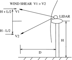
The method is based on monitoring of the evolution of the first harmonic of the signal in the turbine cycle loading, which appears due to the wind shear. Amplitude of the first harmonic is estimated in two ways, which are described as follows: (1)The first harmonic can be extracted from the blade root moment sensor signal, which contains a number of harmonics and a measurement noise. A number of algorithms can be used for estimation of the first harmonic, taking into account a property of persistence of excitation of the blade root moment sensor signal in the presence of the wind shear. This method is associated with processing of the blade load signal using least-squares algorithm with harmonic regressor [17-21] for estimation of amplitude of the first harmonic. (2) LIDAR-enabled blade load estimation opens new opportunities for the model-based blade load sensor fault detection. The first harmonic of the turbine cycle loading can be estimated using upwind speed measurements in multibeam configuration which is illustrated in Figure 1. This method is referred as a model-based blade load estimation method, driven by upwind speed measurements.

Figure 1. Multibeam LIDAR measurements of two wind speeds V1 and V2 (located at the heights which are equal to the hub height H with the half of the blade length L added/subtracted) at a distance D in front of the turbine. A periodic loading appears on the blades with the rotation of the turbine rotor in the presence of a vertical wind shear, which is associated with a change (increase) in wind speed with height, V1 > V2. This periodic loading has a number of harmonics and a first harmonic is associated with the rotational frequency.

Estimation of the first harmonic described above is based on two sensors with different measurement principles, and therefore can be combined for a high performance failure detection. The detection is associated with monitoring of statistical properties of the difference between amplitudes of the first harmonic calculated in two different ways.

Notice that load sensors (strain gauges), located on the fixed part of the nacelle, which measure tilt and yaw nacelle moments, could also be used for estimation of the blade loads via inverse Coleman transformation as is described in [10]. The same measurement principle associated with estimated and measured blade loads together with inaccuracies in Coleman transformation (see [22] for details) result in poor detection performance in this case.

The fault detection method proposed in this paper is associated with a change detection, where the change in parameters of distribution of the difference between amplitudes of the first harmonic identifies the fault.

Three types of faults can be detected: (1) abrupt jump faults with a step-like behavior, where the signal changes abruptly from the nominal value to a faulty value; (2) incipient faults with a drift-like behavior, where the signal gradually changes from the nominal value to a faulty value; (3) intermittent faults, where the signal changes from the nominal value to a faulty value, and returns to the nominal value after some time. All three types of faults can be identified via detection of the changes in the parameters of distribution of the difference between the amplitudes.

Notice that this paper does not cover all types of faults which may appear in a wind turbine. Additional fault scenarios together with a benchmark wind turbine model are presented in [23].

New Detection Method of the Blade Load Sensor Failures

Model of the flapwise bending moment: accounting for higher harmonics

Two wind speeds, measured at different heights, see Figure 1, are the input to the turbine load model. The periodic individual blade wind speeds V_i , i = 1, 2, 3, defined at the center of each blade in rotating frame can be calculated using these two wind speeds (as boundary conditions), which together with the turbine rotor speed ω_r are associated with the individual blade tip-speed ratio λ_i as follows:

${\lambda }_{i}=\omega {\overline {\vee R_{ri}}}$

(1)

where R is the rotor radius. Individual blade wind speeds have a fundamental frequency associated with a turbine rotational speed. The individual blade wind speed together with the pitch angle and rotor speed define the individual blade flapwise bending moment M_f,i , which can be presented as an average value and a periodic component induced by wind shear. This component contains the first harmonic of the turbine rotational frequency and high order harmonics and can be described as follows:

$M_{f,i}=A_{0}+\sum _{h=1}^{d}A_{h,i}cos\left(h{\omega }_{r}t\right)$

(2)

where A₀ = A₀(V, ω_r , β_c ) is the average value of the flapwise bending moment, and A_h,i  = A_h,i (V₁, V₂, ω_r, β_c ) is the amplitude of the harmonic h, where d is a total number of harmonics. The average value of the flapwise bending moment depends on the hub wind speed V, turbine speed ω_r and collective pitch angle β_c . The amplitudes depend on two wind speeds V₁ and V₂, which characterize wind shear, see Figure 1, turbine speed and collective pitch angle.

Notice that wind shear consists of vertical and horizontal components. A vertical component is accounted only in this model as the most pronounced component of the wind shear. A horizontal component, which is not accounted in this model is treated as stochastic variations of the amplitudes.

Processing of persistently exciting blade root moment sensor signal: amplitude estimation

Discrete-time measurements of individual blade flapwise bending moment M_fk (where index i is dropped for simplicity) with d harmonics can be written as follows:

$M_{fk}=\sum _{h=1}^{d}A_{hk}cos\left(h{\omega }_{rk}k\right)+$${\xi }_{k}={\phi }^{T}{\theta }_{{_{\ast }}k}+{\xi }_{k}k$

(3)

where ${\textstyle \varphi }$_k is the harmonic regressor and θ_*k is the vector of unknown parameters defined as follows:

${\begin{array}{rl}{\phi }^{T}&=[cos\left({\omega }_{rk}k\right)cos{\left(2{\omega }_{rk}k\right)}_{k}\\&cos\left(3{\omega }_{rk}k\right)\ldots cos\left(d{\omega }_{rk}k\right)]\end{array}}$

(4)

${\theta }_{k{_{\ast }}}^{T}\left[A_{1k}A_{2k}A_{3k}\ldots A_{2k}\right]$

(5)

where ω_rk is a discretized turbine speed, ξ_k is a zero mean white Gaussian measurement noise, k = 1, 2, … is the step number. Notice that the average value of the flapwise bending moment can be easily estimated using a low-pass filter and subtracted from the individual blade flapwise bending moment signals. Therefore, signal (3) contains the periodic component only. Least-squares estimate:

${\theta }_{k}^{T}=\left[A_{1k}A_{2k}A_{3k}\ldots A_{dk}\right]$

(6)

of unknown parameter vector θ_*k in a window of a size N, which is moving in time, can be written as follows [19]:

${\theta }_{k}={\left[\sum _{j=k-N+1}^{k},{\phi }_{j},{\phi }^{T}\right]}^{-1j}\sum _{j=k-N+1}^{k}{\phi }_{j}M_{f}$

(7)

and the first harmonic M_ffk is recovered according to the relation:

$M_{ffk}=A1_{k}cos\left({\omega }_{k}k\right)$

(8)

where A1k is estimated of the first harmonic.

The matrix ${\textstyle \sum _{j=k-N+1}^{k}{\varphi }_{j}{\varphi }_{j}^{T}}$ is called as information matrix and it is an SDD matrix for a sufficiently large window size [20]. The SDD matrix can easily be inverted making algorithm computationally efficient and implementable. Moreover, estimated parameters can also be rapidly and accurately calculated without matrix inversion [21].

Estimation problem stated above is a challenging estimation problem due to time-varying amplitudes and rotational speed. The accuracy of estimation can be improved via reduction of the window size for fast varying parameters. The properties of the information matrix based on harmonic regressor have not been studied for a sufficiently small window size N. The case, where the window size is not large enough for information matrix to be an SDD matrix is considered in the Appendix. A positive definiteness of the information matrix based on harmonic regressor with four components is shown in this Appendix using the partitioning method.

A measurement noise together with non-stationary nature of estimated parameters and turbine rotational speed are the main obstacles to high performance estimation of the first harmonic of the flapwise bending moment in real-time.

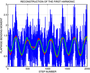
Post-processing estimation, where all the signals are saved in the buffer and future values of the measured signal are available shows significant improvement with respect to real-time estimation (see Fig. 2).

Figure 2. Reconstruction of the first harmonic from a noisy blade load signal in post processing. Measured signal of the flapwise bending moment, which contains four harmonics is plotted with a blue line. The first harmonic is plotted with a green line, and estimate of this harmonic is plotted with a red line. The flapwise bending moment is presented in normalized unit.

Model-based estimation of the amplitude of the first harmonic

Two wind speeds which are measured at a distance in front of the turbine (see Fig. 1) are used for model-based estimation of the amplitude of the first harmonic of blade load. The wind speeds which are expected to arrive to the turbine site after some time can be calculated using a classical frozen turbulence assumption [24]. Expected periodic individual blade wind speeds V_ie , i = 1, 2, 3 defined at the center of each blade in rotating frame can be calculated using two expected wind speeds. Expected periodic individual blade wind speeds together with turbine speed and pitch angle are the inputs to the look-up table, which estimate individual blade flapwise bending moments as follows:

$M_{fm,i}=f\left(V_{ie}\cdot {\omega }_{i}{\beta }_{c}\right)$

(9)

This model is suitable for estimation of first harmonic of turbine rotational frequency only. This harmonic appears in the load in the presence of the wind shear. Amplitude of this harmonic ${\textstyle {\overset {\mbox{ˆ}}{A}}_{1mk}}$ is estimated using least squares method. Notice that two techniques of estimation of the first harmonic described above are based on sensors with different measurement principles and therefore can be combined for high performance failure detection.

Monitoring of the amplitude of the first harmonic: outlier detection

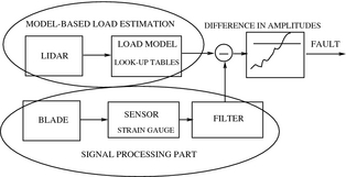
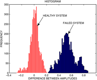
Blade load sensor failure detection mechanism is driven by two sensors: (1) LIDAR, which measures two wind speeds at a distance in front of the turbine, and (2) blade strain gauges, which measure a flapwise bending moment. A chart of the detection mechanism is presented in Figure 3. Two amplitudes of the first harmonic of rotational frequency are estimated and compared. A difference between the amplitudes ${\textstyle \Delta A_{k}={\overset {\mbox{ˆ}}{A}}_{1mk}-{\overset {\mbox{ˆ}}{A}}_{1k}}$ , which is calculated in two ways is normally distributed with a zero mean value for healthy system. The parameters of such distribution can be identified using a sufficiently large number of measured points in the case of a healthy system. The fault detection is associated with a change detection, where the change of the parameters of this distribution identifies the fault.

Figure 3. Detection of blade load sensor faults.

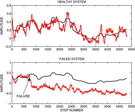
A slow drift of the amplitude of the first harmonic of the strain gauge signal is shown as an example in Figure 4 with corresponding distributions plotted in Figure 5. Such a drift may appear due to the fatigue of the material in the cycle loading or humidity change, which results in a change of gauge factor (see section 'Individual pitch control and unreliable blade load measurements' for all types of faults).

Figure 4. A time chart of the amplitudes of the first harmonic of the healthy system (the first subplot) and a failed system (the second subplot). Amplitudes of the first harmonic calculated using load model and sensor signal are plotted with black and red lines, respectively. Incipient fault associated with a slow drift occurs in step number 700. Histograms of healthy and failed systems are plotted in Figure 5.

Figure 5. Histogram of the difference between the amplitudes of the first harmonic for a healthy system (plotted with red color) and for a failed system, plotted with blue color.

Each sample of the difference between amplitudes should belong to a parent distribution, associated with a healthy system. The fault is detected if the sample is identified as an outlier (outlier is an observation point which is distant from other observations).

An outlier is detected via a two sample t-test, where a hypothesis that a mean value of the distribution that describes a healthy system is equal to the suspected outlier, which is treated as a mean value of a virtual distribution [25], is taken as a null hypothesis. This hypothesis is tested against an alternative hypothesis that the observation point does not belong to the parent distribution that describes the healthy system. The failure is detected if the null hypothesis is rejected in favor of an alternative hypothesis.

A slow drift can also be detected via monitoring of the fluctuations of the mean value of the difference between the amplitudes. This monitoring is performed in a window of a certain size, which is moving in time. Notice that the difference in mean values should be statistically significant for reliable detection of the fault. This can be verified using the two sample t-test, where a significance level represents trade-off between fastness and detection performance.

Adaptation of the Load Model

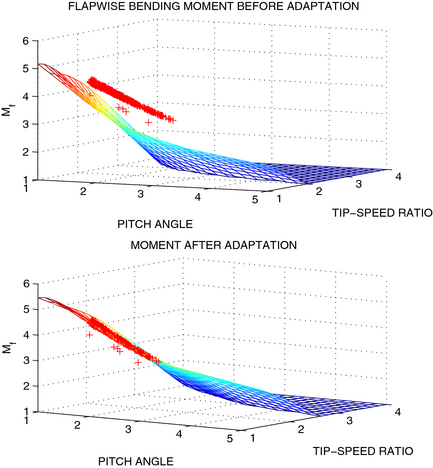
The performance of the detection mechanism, described above, depends on the performance of the load model, which is a mean value model that describes the flapwise blade root bending moment (see Fig. 3). The model of the flapwise bending moment is presented in the form of look-up tables (the surfaces in three-dimensional space) with the tip-speed ratio and blade pitch angle as input variables. The mean value of the bending moment calculated via look-up tables should coincide with the outputs of the blade load sensors in a uniform wind field for the healthy system. Deviations between the load sensor measurements and output of the model necessitate adaptation of the model, provided that the wind field is uniform. The uniformity of the wind speed across the rotor swept area is detected by comparison of the blade load sensor signals of all three blades and/or by LIDAR measurements. Average values of the load calculated using blade load sensors in a number of working points are memorized for adaptation of look-up tables. The data should be acquired over a relatively large time segment to ensure statistical consistency. Notice that additional requirements may be imposed on input data to avoid erroneous adaptation. If new data are available in a certain operating region only (e.g., at low wind speeds and for small pitch angles), then the part of the surface parameters is adapted (e.g., gradient in pitch angle direction). Adaptation of the look-up table is associated with a motion of the surface in three dimensional space (see Fig. 6). The position and orientation of the surface in three-dimensional space change only after adaptation, which in turn allows for a prediction of the bending moment for a wide range of operating variables. This adaptation method was developed first in automotive applications [25] and was successfully applied to turbine model validation with fusion of simulation and measurement data on Big Glenn wind turbine, located outside Gothenburg, Sweden [26].

Figure 6. The flapwise bending moment is presented as a surface with tip-speed ratio and pitch angle as input variables for a certain turbine speed [14]. Mean values of measured flapwise bending moment are plotted with plus signs of a red color. The surface is adapted against measured data, minimizing deviations between the surface and measured points. All variables are presented in normalized units.

Conclusion

Increasing demands on operational reliability, safety, and power output of wind turbines necessitate the development of new high-performance fault detection techniques. High-performance fault detection is directly associated with predictive maintenance [27], where a component is replaced before the system breaks down, which implies significant savings as well as increases power output. Moreover, high performance fault detection methods are the basis for novel fault-tolerant turbine control strategies, where a fault is predictively detected, and the turbine is switched to a safe operation mode to prevent damages, until a maintenance crew arrives at the turbine site. This extends the turbine operation time and increases the power output. Fault tolerance is associated with an ability of the turbine control system to maintain control objectives, despite the occurrence of a fault [28-30]. New blade load sensor fault detection technique proposed in this paper is the basis for high performance fault-tolerant IPC. This is also a new application for future multibeam LIDAR technology, which is utilized now in the preview-based control only. New detection algorithms can be easily integrated into existing IPC functionality aiming for improvement of uneven load reduction for large turbines.

Acknowledgments

This work was supported by ÅF. The author is grateful to WindVector AB and Albert Santiago from Avent Lidar Technology for interesting discussions about multibeam LIDAR technologies.

Conflict of Interest

None declared.

Appendix

Positive Definiteness of Information Matrix for Insufficiently Large Window Size: Partitioning Method for the Case of Four Harmonics

Consider the following harmonic regressor:

${\phi }^{T}={\left[cos\left(\omega k\right)cos\left(2\omega k\right)cos\left(3\omega k\right)cos\left(4\omega k\right)\right]}_{k}$

(A1)

where ω is a constant rotational frequency and hω with h = 2, 3, 4 are higher harmonics, k = 1, 2, … is the step number. Consider the following information matrix calculated over the window of a size N:

$G=G^{T}=\sum _{k=1}^{N}{\phi }_{k}{\phi }_{k}^{T}=\left[{\begin{array}{cccc}g_{11}&g_{12}&g_{13}&g_{14}\\g_{12}&g_{22}&g_{23}&g_{24}\\g_{14}&g_{24}&g_{34}&g_{44}\end{array}}\right]$

Elements of the matrix G can be evaluated explicitly using the following relation:

$\sum _{k=1}^{N}cos\left(h\omega k\right)={\frac {cos(N+1b\omega )}{2}}sin{\frac {\left(Nh\omega \right)}{2}}sin\left({\frac {hw}{2}}\right)$

(A2)

where h = 1, …, 4. The first two elements of the first row of this matrix are presented below:

$g_{11}=\sum _{k=1}^{N}{cos}^{2}\left(\omega k\right)={\underset {average\quad part}{\underbrace {\frac {N}{2}} }}+$${\underset {periodic\quad part}{\underbrace {\frac {sin(N\omega )cos((N+1)\omega )}{2sin\omega }} }}$

${\begin{array}{rl}g_{12}&=\sum _{k=1}^{N}cos\left(\omega k\right)cos\left(2\omega k\right)\\&={\frac {1}{2}}cos\left({\frac {3(N+1)}{2}}\right)\omega sin\left({\frac {3N\omega }{2}}\right)sin\left({\frac {3\omega }{2}}\right)\\&={\frac {1}{2}}cos\left({\frac {N+1}{2\omega }}\right)sin\left({\frac {3\omega N}{2\omega }}\right)sin\left({\frac {\omega }{2}}\right)\end{array}}$

(A3)

All other elements of this matrix can be evaluated using similar arguments.

Partitioning of Matrix G

Symmetric matrix G can be partitioned as follows:

${\begin{array}{c}\left[A,B\right]\\G=B^{T}C\end{array}}$

where

$A=\left[{\begin{array}{cc}g_{11}&g_{12}\\g_{21}&g_{22}\end{array}}\right]\quad B=\left[{\begin{array}{cc}g_{33}&g_{34}\\g_{34}&g_{44}\end{array}}\right]$

$C=\left[{\begin{array}{cc}g_{13}&g_{14}\\g_{23}&g_{24}\end{array}}\right]$

Notice that the diagonal elements of the matrices A and C have periodic part and average part N/2, whereas all other elements of matrices A, B and C have periodic parts only. Matrix G becomes an SDD matrix for a sufficiently large window size N. Suppose that the window size N is large enough for matrices A and C to be SDD matrices, but it is not sufficiently large for matrix G to be an SDD matrix. The matrix G is positive definite if and only if the matrices A and C − B^TA⁻¹B are positive definite matrices (see theorem 7.7.6 in [31]). Inverse of the matrix A can be approximated as ${\textstyle A^{-1}\approx D={\frac {2}{N}}I}$ , when neglecting periodic part in matrix A, where I is the identity matrix. The matrix ${\textstyle B^{T}B}$ also has an average part that is proportional to the window size N. This part is canceled by the diagonal elements of matrix D in the term B^TA⁻¹B. Therefore there exists a large enough window size N such that the matrix C − B^TA⁻¹B is an SDD matrix. Hence the matrix G is a positive definite matrix, since matrix A is also an SDD and positive definite matrix. Notice that the matrix G is not an SDD matrix.

This technique of determination of positive definiteness of information matrix is illustrated via numerical example in the next Section.

Numerical example

Consider the following information matrix G based on the regressor equation (A1) with ω = 0.0228 and the window size N = 83:

$G=\left[{\begin{array}{cccc}34.4747&16.2691&-1.9465&-4.8693\\16.2691&46.5787&19.8127&-10.6043\\-1.9465&19.8127&37.9209&22.3866\\-4.8693&-10.6043&22.3866&42.5117\end{array}}\right]$

This matrix G is not an SDD matrix since the diagonal elements in the second and the third rows are not larger than the sum of the magnitudes of all the other (non-diagonal) entries in the second and third rows. Nevertheless, the matrices ${\textstyle A=\left[{\begin{array}{cc}34.4747&16.2691\\16.2691&46.5787\end{array}}\right]}$ and ${\textstyle C-B^{T}A^{-1}B=\left[{\begin{array}{cc}26.7629&26.5384\\26.5384&40.0503\end{array}}\right]}$ are positive definite and SDD matrices. Therefore the matrix G is a positive definite matrix. Notice that the matrices A and C−B^TA⁻¹B are still positive definite (but not SDD) matrices even for a sufficiently small window size N.

References

1. Bossanyi, E. 2003. Individual blade pitch control for load reduction. Wind Energy6: 119–128.
2. Larsen, T., H. Madsen, and K. Thomsen. 2005. Active load reduction using individual pitch, based on local blade flow measurements. Wind Energy8:67–80.
3. Stol, K., W. Zhao, and A. Wright. 2006. Individual blade pitch control for the Controls Advanced Research Turbine (CART). J. Sol. Energy Eng.128:498–505.
4. Selvam, K., S. Kanev, J. van Wingerden, T. van Engelen, and M. Verhaegen. 2009. Feedback-feedforward individual pitch control for wind turbine load reduction. Int. J. Robust Nonlinear Control19:72–91.
5. Lackner, M., and G. van Kuik. 2010. A comparison of smart rotor control approaches using trailing edge flaps and individual pitch control. Wind Energy13:117–134.
6. Jelavic, M., V. Petrovic, and N. Peric. 2010. Estimation based individual pitch control of wind turbine. Automatika51:181–192.
7. Bossanyi, E., P. Fleming, and A. Wright. 2013. Validation of individual pitch control by field tests on two- and three-bladed wind turbine. IEEE Trans. Control Syst. Technol.21:1067–1078.
8. Petrovic, V., and F. Campagnolo. 2013. Pp. 472–477inExperimental validation of wind turbine higher harmonic control using shaft loads measurements. European Control Conference (ECC), Zurich, Switzerland, 17–19 July 2013.
9. Stotsky, A., and B. Egardt. 2013. Individual pitch control of wind turbines: model-based approach. Proc. Inst. Mech. Eng. Part I: J. Syst. Control Eng.227:602–609.
10. Wei, X., M. Verhaegen, and T. van Engelen. 2008. Sensor fault diagnosis of wind turbines for fault tolerant. Pp. 3222–3227 in Proceedings of the 17th World Congress, The International Federation of Automatic Control, Seoul, Korea, 6–11 July 2008.
11. Johnson, K., L. Pao, M. Balas, and L. Fingersh. 2006. Control of variable-speed wind turbines: standard and adaptive techniques for maximizing energy capture. IEEE Control Syst. Mag.26:70–81.
12. Laks, J., L. Pao, A. Wright, N. Kelley, and B. Jonkman. 2011. The use of preview wind measurements for blade pitch control. Mechatronics21:668–681.
13. Wang, N., K. Johnson, and A. Wright. 2012. FX-RLS-based feedforward control for LIDAR-enabled wind turbine load mitigation. IEEE Trans. Control Syst. Technol.20:1212–1222.
14. Stotsky, A., B. Egardt, and O. Carlson. 2013. An overview of proactive wind turbine control. Energy Sci. Eng.1:1–10.
15. Wagenaar, J., S. Davoust, A. Medawar, G. Coubard-Millet, and K. Boorsma. 2014. Turbine performance validation: the application of Nacelle LIDAR, EWEA, Barcelona, Spain, 10–13 March 2014.
16. Klasen, L. 2014. Lidar systems for wind energy applications. Pp. 97–100in Proceeding of Swedish Society of Automated Image Analysis, Symposium on Image Analysis, Luleå, 11–12 March 2014.
17. Ioannou, P., and J. Sun. 1996. Robust adaptive control. Prentice-Hall, Englewood Cliffs, NJ.
18. Bayard, D.2000. A general theory of linear time-invariant adaptive feedforward systems with harmonic regressors. IEEE Trans. Autom. Control45:1983–1996.
19. Ljung, L.1999. System identification: theory for the user. Prentice-Hall, Upper Saddle River, NJ.
20. Stotsky, A.2010. Recursive trigonometric interpolation algorithms. Proc. Inst. Mech. Eng. Part I: J. Syst. Control Eng.224:65–77.
21. Stotsky, A. 2013. Robust least-squares estimation with harmonic regressor: high order algorithms. Pp. 6516–6521in 52nd IEEE Conference on Decision and Control, Florence, Italy, 10–13 December 2013.
22. Bir, G. 2008. Multiblade coordinate transformation and its application to wind turbine analysis, Preprint NREL/CP-500-42553 January 2008.
23. Odgaard, P., J. Stoustrup, and M. Kinnaert. 2013. Fault-tolerant control of wind turbines: a benchmark model. IEEE Trans. Control Syst. Technol.21:1168–1182.
24. Taylor, G.1938. The spectrum of turbulence. Proc. R. Soc. Lond.164:476–490.
25. Stotsky, A.2009. Automotive engines: control, estimation, statistical detection. Springer, Berlin, Heidelberg.
26. Stotsky, A. Wind turbine model validation: fusion of simulation and measurement data, 19-th IFAC World Congress, Capetown, South Africa, 22–29 August 2014 (forthcoming).
27. Bertling, L. 2002. Reliability centred maintenance for electric power distribution systems. Doctoral Thesis KTH, Stockholm, Sweden, ISBN 91-7283-345-9.
28. Esbensen, T., and C. Sloth. 2009. Fault diagnosis and fault-tolerant control of wind turbines. Technical Report, Faculty of Engineering, Science and Medicine, Department of Electronic Systems, Section for Automation and Control, Aalborg University, Denmark.
29. Pourmohammad, S., and A. Fekih. 2011. Fault-tolerant control of wind turbine systems – a review, Proceeding of Green Technologies Conference (IEEE-Green), 2011 IEEE, Baton Rouge, LA, 14–15 April 2011.
30. Rezaei, V., and K. Johnson. 2013. Robust fault tolerant pitch control of wind turbines. Pp. 391–396in 52nd IEEE Conference on Decision and Control, Florence, Italy, 10–13 December 2013.
31. Horn, R., and C. Johnson. 1985. Matrix analysis, Cambridge Univ. Press, Cambridge, U.K.

References

1. Bennion, B., and S. Bachu. 2008. Drainage and imbibition relative permeability relationships for supercritical CO₂/Brine and H₂S/Brine systems in intergranular sandstone, carbonate, shale and anhydrite rocks. SPE Res. Eval. & Eng.11:487–496. Available at http://dx.doi.org/10.2118/99326-PA.
2. Bennion, B., and S. Bachu. 2005. Relative permeability characteristics for supercritical CO₂ displacing water in variety of potential sequestration zones in the western Canada sedimentary basin. SPE 95547, SPE annual technical conference, Dallas, Texas, US, Available at http://dx.doi.org/10.2118/95547-MS.
3. IPCC. 2005. Special report on carbone dioxide capture and storage, published for the intergovernmental panel on the climate change. Cambridge University Press, Printed in Canada.
4. Krause, M., J. C. Perrin, and S. M. Benson. 2011. Recent progress in predicting permeability distribution for history matching core flooding experiments. Energy Procedia4:4354–4361. Available at http://dx.doi.org/10.1016/j.egypro.2011.02.387.
5. Pini, R., S. C. M. Krevor, and S. M. Benson. 2012. Capillary pressure and heterogeneity for the CO₂-brine system in sandstone rocks at reservoir conditions. Adv. Water Res.38:48–59. Available at http://dx.doi.org/10.1016/j.advwatres.2011.12.007.
6. Soroush, M., D. Wessel-Berg, O. Torsaeter, and J. Kleppe. 2013. Investigating impact of flow rate and wettability on residual trapping in CO₂ storage in brine through relative permeability experiments. Energy Environ. Res. J.3:53–72. Available at http://dx.doi.org/10.5539/jgg.v3n2p53.
7. Chang, Y. B., M. T. Lim, G. A. Pope, and K. Sepehrnoori. 1994. CO₂ flow patterns under multiphase flow: heterogeneous flied scale conditions. SPE Reservoir Eng.9:208–216. Available at http://dx.doi.org/10.2118/22654-PA.
8. Sasaki, K., S. Akibayashi, N. Yazawa, Q. T. Doan, and S. M. Farouq Ali. 2001. Experimental modeling of the SAGD process - enhancing SAGD performance with periodic simulation of the horizontal producer. SPE J.6:89–97. SPE-69742-PA, Available at http://dx.doi.org/10.2118/69742-PA.
9. Cinar, Y., K. Jessen, R. Berenblyum, R. Juanes, and F. M. Jr Orr. 2006. An experimental and numerical investigation of crossflow effects in two phase displacement. SPE J.11:216–226, SPE-90568-PA, Available at http://dx.doi.org/10.2118/90568-PA.
10. Lenormand, R., E. Touboul, and C. Zarcone. 1988. Numerical models and experiments on immiscible displacement in porous media. J. Fluid Mech.189:165–187. Available at http://dx.doi.org/10.1017/S0022112088000953.
11. Cinar, Y., A. Riaz, and H. A. Tchelepi. 2009. Experimental study of CO₂ injection into saline formations. SPE J.14:588–594. SPE-110628-PA, Available at http://dx.doi.org/10.2118/110628-PA.
12. Polak, S., Y. Cinar, T. Holt, and O. Torsaeter. 2009. An experimental investigation of the balance between capillary, viscous and gravitational forces during CO₂ injection into the saline aquifers. Energy Procedia4:4395–4402. Available at http://dx.doi.org/10.1016/j.egypro.2011.02.392.
13. Gonzalez, C. R., E. R. Woods, and L. S. Eddins. 2009. Digital image processing using MATLAB, 2 ed. Gatemark Publishing. ISBN:978-0-9820854-0-0. Available at: www.gatesmark.com
14. Young, T. I., J. J. Gerbrands, and J. L. Van Vliet. 1998. Fundamentals of image processing. Delft University of Technology Publishing, Netherland, ISBN: 90-75691-01-7.
15. Soroush, M., D. Wessel-Berg, and J. Kleppe. 2013. Effects of wetting behaviour on residual trapping in CO₂-brine systems. SPE-165334-MS, SPE Western Regional & AAPG Pacific Section Meeting, Joint Technical Conference, Monterey, CA. Available at http://dx.doi.org/10.2118/165334-MS.
16. Gupta, S. P., and S. P. Trushenski. 1979. Micellar flooding of compositional effects on oil displacement. Soc. Pet. Eng. J.19:116–28. Available at http://dx.doi.org/10.2118/7063-PA.
17. Iffly, R., D. C. Rousselet, and J. L. Vermeulen. 1972. Fundamental study of imbibition in fissured oil fields. SPE 4102. 47th Annual technical Conference of SPE, San Antonio, TX. Available at http://dx.doi.org/10.2118/4102-MS.
18. Soroush, M., D. Wessel-Berg, and J. Kleppe. 2013. Investigating residual trapping mechanism in CO₂ storage in the brine through analytical and numerical simulation methods. SPE-164804-MS, EAGE Annual Conference & Exhibition incorporating SPE Europec held in London, United Kingdom. Available at http://dx.doi.org/10.2118/164808-MS.
19. Land, C. S. 1971. Comparison of calculated with experimental imbibition relative permeability. SPE J.11:419–425. Available at http://dx.doi.org/10.2118/3360-PA.
20. Killough, J. E. 1976. Reservoir simulation with history-dependent saturation functions. SPE J.16:37–48. Available at http://dx.doi.org/10.2118/5106-PA.
21. Kleppe, J., P. Delaplace, R. Lenormand, G. Hamon, and E. Chaput. 1997. Representation of the capillary pressure hysteresis in reservoir simulation. SPE 38899, presented at SPE annual conference and exhibition, San Antonio, US, Available at http://dx.doi.org/10.2118/38899-MS.
22. Carlson, F. M. 1981. Simulation of relative permeability hysteresis to the non-wetting phase. SPE10157, SPE Annual Technical Conference and Exhibition, San Antonio, Texas, Available at http://dx.doi.org/10.2118/10157-MS.
23. Schlumberger eclipse technical description. 2012. Schlumberger eclipse technical description. Available at http://www.slb.com, Visited in summer 2013.
24. Hebach, A., A. Oberhof, N. Dahmen, A. Kogel, H. Ederer, and E. Dinjus. 2002. Interfacial tension at elevated pressures, measurements and correlations in water+carbon dioxide system. J. Chem. Eng.47:1540–1546. Available at http://dx.doi.org/10.1021/je025569p.
25. Chequet, P., J. L. Daridon, D. Broseta, and S. Thibeau. 2007. CO₂/water interfacial tensions under pressure and temperature conditions of CO₂ geological storage. Energy Convers. Manage.48:736–744. Available at http://dx.doi.org/10.1016/j.enconman.2006.09.011.
26. Silin, D., T. Patzek, and S. M. Benson. 2009. A model of buoyancy-driven two-phase countercurrent fluid flow. Transp. Porous Media76:449–469. Available at http://dx.doi.org/10.1007/s11242-008-9257-1.
27. Bentsen, R. G., and J. Anli. 1977. Using parameter estimation techniques to convert centrifuge data into a capillary pressure curve. SPE J.17:57–64. Available at http://dx.doi.org/10.2118/5026-PA.
28. Spencer, D. A. 1973. P. 574inThe focal dictionary of photographic technologies. Focal Press, Prentice-Hall, University of Michigan, Ann Arbor, MI. ISBN 9780133227192.
29. Nordbotten, J. M., M. A. Celia, and S. Bachu. 2005. Injection and storage of CO₂ in deep saline aquifers: analytical solution for CO₂ plume evolution during injection. Transp. Porous. Med.58:339–360. Available at http://dx.doi.org/10.1007/s11242-004-0670-9.
30. Micheal, K., G. Allinson, A. Golab, S. Sharma, and V. Shulakova. 2009. CO₂ storage in saline aquifers II, experience from existing storage operations. Energy Procedia1:1973–1980. Available at http://dx.doi.org/10.1016/j.egypro.2009.01.257.
31. Kopp, A., H. Class, and R. Helmig. 2009. Investigations on CO₂ storage capacity in saline aquifers part 1. Dimensional analyses of flow processes and reservoir characteristics. Int. J. Greenhouse Gas Control3:263–276. Available at http://dx.doi.org/10.1016/j.ijggc.2008.10.002.
32. Singh, V., A. Cavanaghm, H. Hansen, B. Nazarian, M. Iding, and P. Ringrose. 2010. Reservoir modeling of CO₂ plume behavior calibrated against monitoring data from Sleipner, Norway, SPE 134891, and Presented at SPE annual conference and exhibition held in Florence, Italy, Available at http://dx.doi.org/10.2118/134891-MS.
33. Rumpf, H., and A. R. Gupte. 1975. The influence of porosity and grain size distribution on the permeability equation of porous flow. Chemie Ing. Techn. (Weinheim)43:367–375.