
Section: Earth and Space Science
Performers:
Candidate of Physical and Mathematical Sciences, Department of FTT and NF of Al-Farabi KazNU.Dr. Alimgazinova N.Sh.
1.1 Solar flares 5
1.2 Energy release during solar flares 6
1.3 The impact of Solar Activity on Earth 6
2.1 Information entropy 8
2.2 Two-dimensional shape factor 8
3.1 Solar flare and sunspot data 8
3.1.5 Solar flares in sunspot group #3186 8
3.2 Information-entropy analysis of solar flare signals 8
ANNOTATION
Scientific research project consists of 15 pages, including 17 pictures, 8 tables and the list of 11 literature references.
The key words: Solar flares, information, entropy, X-Rays, two-dimensional shape factor.
The goal of the research project – to apply information-entropy analysis to study and identify the features of the Sun's X-ray radiation signals in different periods of solar activity.
The task of the research – to study the second fluxes of X-ray radiation according to the GOES-16 spacecraft data in different periods of solar activity.
The objects of the research – the solar X-ray fluxes for events that took place from 2017 to 2023.
The methods of the research – the information-entropy analysis.
Steps of analysis:
- 1. The literature review for Sun and Solar activities
- 2. Analysis of Solar flare’s data and creation of the researched events’ list to be studied.
- 3. Getting familiar with variety of application software packages for the research.
- 4. Development of programs for constructing time diagrams of solar radiation signals and for calculating nonlinear characteristics.
- 5. Schematic diagrams construction and calculation of nonlinear characteristics. Analyzing the obtained results.
Degree of independency – performed independently.
The results – During the research 10 solar flares events has been analyzed. The deep analysis of the sunspots group, where the solar activity has happened, was performed for each solar flare event. The Shannon information entropy and two-dimensional shape factor were calculated, which showed the features of the signals at different time periods.
INTRODUCTION
The Sun is the center of the Solar System, which is a sphere of hot, electrically charged gas, plasma. It plays a huge role in the life of all living things. The Sun's rays travel the distance to Earth in 8 minutes, making anomalies easy to spot, even feel. This proximity makes the Sun the only star we see not as a point but as a disc. All these facts speak to the importance of studying the Sun.
Observations of the Sun provide a large amount of valuable information and numerical data, which in the future may be useful in predicting various anomalies and then preparing to prevent their effects. The largest processes occurring at the surface of the solar atmosphere are solar flares. Flares are sudden and brief bursts of activity on the Sun, accompanied by the release of enormous amounts of energy, the scale of which is equivalent to the explosion of a million hydrogen bombs. These bright and dynamic events have significant consequences for our planet and the surrounding cosmic space. In this research paper, we focus on the study of the patterns of solar flares and their impact on the environment [1].
CHAPTER 1. SOLAR ACTIVITY
1.1 Solar flares
A solar flare is an explosion of plasma that causes the release of a large amount of energy in the chromosphere (the lower part of the Sun's corona), a region with unstable magnetic fields. The magnetic field causes a strong compression of the solar plasma, resulting in the formation of a flagellum (plasma streak), which is accompanied by an explosion. Explosions are often accompanied by coronal mass ejections. The released energy of the explosion ranges from 1020 J (weak flares) to 1025 J (strong flares). In the explosion zone, the plasma heats up to 10 million K. The energy of the matter ejected into interplanetary space increases. Streams of charged particles such as electrons and protons are accelerated by the released energy. Radio waves and gamma rays are amplified.
Most solar flares consist of emission lines of hydrogen atoms and ions, neutral helium, ionized helium, and calcium. During a flare, the solar wind intensifies, ejecting a mass of high-energy particles and plasma. Also, magnetic energy is converted into heat and particles that accelerate the energy to form a corpuscular flux.
To distinguish flares, a taxonomy based on a series of homogeneous measurements using engineering space systems (ESS) is used to measure the amplitude of thermal X-ray bursts in the energy range 0.5-10 keV (corresponding to a wavelength range of 0.5-8 angstroms). The classification depends on the intensity of the X-ray peak achieved by the burst [4].
| Class | Peak flux range (W/m2) |
| A | <10−7 |
| B | 10–7 -10–6 |
| C | 10–6–10–5 |
| M | 10–5–10–4 |
| X | >10−4 |
1.2 Energy release during solar flares
A solar flare is the most powerful manifestation of the Sun's activity. The energy released in a large flare is about a hundred times greater than the thermal energy that can be obtained by burning all known oil and coal reserves on Earth. This enormous energy is released in the Sun over a period of a few minutes, corresponding to an average output during a flare of about 1029 erg/s.
The source of the flare energy is the magnetic field in the Sun's atmosphere. It determines the shape and energy of the active region in which the flare occurs. In this region, the energy of the magnetic field greatly exceeds the thermal and kinetic energy of plasma. During a flare, the excess magnetic field energy is rapidly converted into particle energy and changes the properties of the plasma. The physical process responsible for this conversion is called magnetic reconnection.
1.3 The impact of Solar Activity on Earth
Being not so far away, the Sun has a significant impact on the third planet orbiting it every second. It is generally believed that its emissions stimulate cancer and other skin diseases, malfunctions in magnetic and radio devices, fires, and auroras. And this is indeed true, because during solar flares, a huge flow of energy is released, bringing with it the occasional ejection of matter, optical, X-ray, gamma-ray, and radio emissions. However, solar flares should not be confused with another phenomenon we know of, coronal mass ejection. The processes can sometimes occur simultaneously, resulting in a huge cloud of coronal plasma being ejected into space at a speed of millions of kilometers per hour.
Solar flares, bring to Earth particles of different speeds, which reach the atmosphere in 2-4 days, namely alpha particles, beta particles, protons, electrons, neutrons, and positrons. Due to the planet's magnetic field, many of them are stopped in the Earth's upper atmosphere. In addition, the process involves electromagnetic radiation that travels the distance to Earth in 8 minutes and reaches speeds of 300,000 kilometers per second. The effects of individual solar flares can remain for weeks.
In addition to providing oxygen to living beings, the Earth's atmosphere also fulfils a protective function against cosmic radiation. As a result, most of the exposure to radiation is in the upper atmosphere, thereby affecting passengers and personnel in aircraft flying over the polar zone, astronauts in outer space, and radio waves. Thus, powerful X-class flares can disrupt radio communications worldwide, while weaker M-class flares can temporarily disable radio devices, especially in polar regions. Also, when accompanied by coronal ejections, strong magnetic storms occur, leading to disruption of electrical equipment, overloading or disabling power grids, resulting in massive power outages, if technical companies are unprepared.

For example, we can mention the effects of the strongest solar flare in history, leading to a terrifying geomagnetic storm in 1859, known as the Carrington Event. Official sources reported northern lights in every corner of the planet, including Cuba, southern Japan and even the equator. Telegraph lines and power grids were overloaded from the electric current flowing through the wires, causing electric shocks and paper catching fire.
If such a phenomenon were to occur again today, it would lead to a prolonged decrease in total ozone content, causing significant global cooling, for example a temperature drops in Europe of up to five degrees centigrade. Such a storm could have catastrophic consequences for mobile and satellite communications, the Internet, and the global energy system [6].
2 CHAPTER. INFORMATION-ENTROPIC ANALYSIS
The Sun is one of the objects of a nonlinear open system that exchanges energy, matter, and information with the world outside of them, which are included in its radiation streams. The Sun's radio emission provides data on symmetry breaking, structuring and probabilistic behaviour.
In the course of natural structuring, the transition of a system from absolute chaos to order, i.e., self-organisation, is common. This process can be described by two main principles - information and entropy. At the moment there is only one approach to the solution of this issue in science - entropic method, because it is entropy that represents the measure of measuring the chaotic process. There are a number of theses formulated by L. Boltzmann, I. Prigozhin, and J. Klimontovich on the study of entropy evolution. At first, Boltzmann's H-theorem was verbalised, stating that entropy in a closed system can either grow or remain unchanged. With the subsequent development of this branch of science, it was announced in Prigozhin's theorem that in the process of self-organisation entropy generation is minimal. Further, thanks to Klimontovich's S-theorem, it was revealed that entropy in such a case is not generated at all, but on the contrary decreases, which can be seen when comparing the same values of average energy. Nevertheless, these theorems did not provide quantitative indicators of self-organization of complex systems. Just such quantitative information-entropy criteria were first considered in the works of Z.J. Zhanabayev, 1996, the results of which are given below.
2.1 Information entropy
Considering the international terminology, the information Ii obtained at the origin (destruction) of a certain structure with probability Pi is presented at the bottom:
There is also an average of its value, i.e. a measure of uncertainty or information entropy:
In the theory of open systems, information entropy is a priority part, serving as a quantitative value of uncertainty in statistical characterisation, as a value of diversity in the theory of evolution, and as a relative measure of the order of non-equilibrium states in open systems.
One of the remarkable ubiquitous properties of independently persisting systems is the imitation and self-similarity of their hierarchical levels, i.e. a small part of the system contains all its information. Self-similarity or repetition of the same properties on different ranges can be explained as equality of values of some function to its argument. For this reason, for the following calculations of self-similarity criteria, the values of probability P(I) and information entropy S(I) will be taken from fixed points.
Only these fixed points can be called stable, since they are also a mapping of the limit tending to infinity of the function, regardless of the initially taken value of the information:
To describe the ubiquitous natural regularities, were calculated the numbers, which, as mentioned above, are taken from fixed points. To summarise, if the result obtained in the calculations falls within the interval I10≤S≤I1, then the structure can be called self-similar. If the result obtained in the interval I20≤S≤I2, the sought complex structure will be self-organising. The above-mentioned values I10, I20 are the result of the first approximation when decomposing the functions P(I), S(I) into Taylor series:

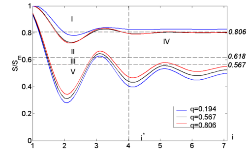

Based on the above figure, depending on the results of calculations of information entropy and two-dimensional shape coefficient, the processes can be divided by type into several groups: processes entering the 12px region can be called noise-like, processes in the 12px region self-similar, in 18px - self-affine, in 18px self-organised and 12px inhomogeneous.
2.2 Two-dimensional shape factor
The two-dimensional shape factor represents the value of the dependence of the change of topological characteristics of entropy, i.e. its continuity, on the change of metric data. Below is written Gelder's integral inequality for random functions , which, due to the use of the generalised metric coefficient, is written as an equality:
This formula will be valid for any integer and fractional values of p, q and is a consequence of the existence of metric characteristics of the values xi(t), xj (t). Based on the topological dimension of the Euclidean surface, the expression, which also corresponds to the Cauchy-Bunyakovsky inequality, should always work.
Thus, given xi = x, xj = 1, p = q = 2, in the calculations we obtain the two-dimensional shape factor of our test signal, which is often used in radio physics.
Provided, xi = x(t), xj = t, we can obtain the affinity features, that is, the heterogeneity of the taken signal. Also, to describe the quantitative qualities of the pattern of dynamic chaos, we can use the mutually established relation between metric features and metric-topological features, that is, between the obtained information-entropic criteria of self-similarity and self-affinity.
CHAPTER 3. RESEARCH RESULTS
Solar flares are divided into five classes depending on the power of X-ray radiation: A, B, C, M, X. The minimum class A (0.0) corresponds to a radiation power in Earth's orbit of ten nanowatts per square meter. As we move to the next letter, the power increases by ten. Therefore, in this study, we selected the most significant long solar flares of M and X classes that have the greatest impact on Earth.
The study used data from ten solar flare events from 2017 to 2023 that differ from the others in energy output (Table 1). Studying the most significant solar flares over the last 5 years on the website [8], we selected the longest flares whose fluctuations will be simpler to track in the graphs.
| № | Classification of Solar Flare | Date | Sunspot Group | Start, UT | Maximum, UT | End, UT |
| 1. | X9,3 | 06.09.2017 | 2673 | 11:53 | 12:02 | 12:10 |
| 2. | Х1.59 | 03.07.2021 | 2838 | 14:18 | 14:29 | 14:34 |
| 3. | X1.1 | 28.10.2021 | 2887 | 15:17 | 15:35 | 15:48 |
| 4. | X2.25 | 20.04.2022 | 2992 | 03:41 | 03:57 | 04:04 |
| 5. | Х1 | 10.01.2023 | 3186 | 22:39 | 22:47 | 22:52 |
| 6. | X1.2 | 29.03.2023 | 3256 | 02:18 | 02:33 | 02:40 |
| 7. | X1.3 | 30.03.2022 | 2975 | 17:21 | 17:37 | 17:46 |
| 8. | M4.4 | 29.11.2020 | 2790 | 12:34 | 13:11 | 13:41 |
| 9. | M1.1 | 29.05.2020 | 2764 | 07:13 | 07:24 | 07:28 |
| 10. | M4.79 | 28.08.2021 | 2860 | 05:39 | 06:11 | 06:23 |
3.1 Solar flare and sunspot data
One method that is used to predict large solar flares is to analyse their sunspots. In the paragraph below we briefly analyse 1 of our 10 selected flares and their sunspots to show the pattern used for predictions.
3.1.5 Solar flares in sunspot group #3186
| Date | Number of sunspots | Size | Sunspot’s Magnitude Classification | Sunspot’s Zürich/Macintosh Classification | Coordinates |
| 10.01.2023 | 5 | 100 | β-δ | DSO | N25E65 |
| 11.01.2023 | 9 | 150 | β-δ | DAI | N24E52 |
| 12.01.2023 | 19 | 320 | β-γ | EKC | N25E38… |
The fifth outburst we are considering, occurred relatively recently, namely on 10 January 2023, having a magnitude of X1, being in spot group 3186 at 11 o'clock at night. This spot group lasted for 13 days, changing its size from 180 million square kilometres to 1522 million square kilometres (in square degree measure 1.2-10.4). The class of spot groups by magnitude class was constantly changing to all kinds of variants, as well as the classification according to the Zürich/Macintosh system (Table 2).
Looking at this date in more detail, the West-North location of the 3186 spot group can be determined at coordinates N25E65, having a size of 304 million square kilometres or 2.1 square degrees (Figure 4)

Although it appears from Figure 3 that the possible effect of radio emissions could have reached the R3 level in strength, this did not happen. The reason lies in the location of the flare, which was at the edge of the spectrum visible to us, due to which also the trajectory of the flare's waste propagation did not pass the Earth, thus not causing any radio storms.
Lastly, judging from the magnetogram in Figure 4 and the information provided in Table 2, the magnetic structure of the 10 January spot group is β-δ, in magnitude class, and DSO according to the Zürich/Macintosh system. Thus, the occurrence of an X-class flare was likely, due to the rather enormous size, the presence of not only a beta magnetic configuration with bipolar spots, but also delta spots.


3.2 Information-entropy analysis of solar flare signals
The time X-ray fluxes were taken from the data archive [5], which contains observational data from the GOES-16 spacecraft.
After storing second-by-second data on X-ray fluxes at time periods that correspond to events of X-class flares that fit our criteria, this information was processed in Spyder (an integrated development environment in the Python programming language used for scientific calculations), using the code given in Appendix 2. Using this programme, we extracted numerical information in the form of tables, i.e. data on XRS-A, XRS-B streams and event timing parameters - TIMES. To clarify, TIMES serves for the temporal characterisation of flashes, while the XRS-A format stores data on radio emission with wavelengths of 0.05-0.4 nm and XRS-B in the range 0.1-0.8 nm. It is the above values that will help to identify the entropy and two-dimensional shape factor, to address the main question of the science project. However, firstly we need to prepare the characterisations for further work.
Figure 5- An example of a graph of solar activity per day
Next, we plotted the time plots for each event in Matlab and highlighted the signals that correspond to the periods of solar flares, as well as the periods before and after solar flares within 5 minutes.
After extraction of the signals, we used a programme that, based on the data entered into it, processes the solar flare data, determines their non-linear characteristics and plots them accordingly.
Table 3 presents the results of the study. As can be seen from the table, during the periods of flares, entropy has values lying in the region of self-organisation and large values of the two-dimensional shape factor. This suggests that this process is regular in its sequence. Each component of the signal is related to the subsequent one, i.e. the realisation of the signal itself depends on the previous development of the event. In the periods 5 minutes before the flashes for the 6 events, the entropy has values greater than in the periods after the flash. The values of the two-dimensional shape coefficient in the periods before and after solar flares are almost identical and have values equal to 1, which indicates that currently simple in shape signals are observed, the changes of which do not differ much from the background radiation of the Sun. During these periods, the signal components do not depend on each other.
| Date | Class | Entropy before | Coefficient of shape before | Entropy of the flare | Coefficient of shape of the flare | Entropy after | Coefficient of shape after | |
| 09.06.2017 | X9.3 | 0.7680 | 1.0012 | 0.7847 | 2.1590 | 0.6818 | 1.0003 | |
| 10.01.2023 | X1 | 0.7555 | 1.0022 | 0.9382 | 1.4184 | 0.7079 | 1.0006 | |
| 29.03.2023 | X1.27 | 0.5228 | 1.0088 | 0.8275 | 2.3760 | 0.6516 | 1.0053 | |
| 30.03.2022 | X1.3 | 0.5310 | 1.0000 | 0.6429 | 2.8271 | 0.5534 | 1.0001 | |
| 03.07.2021 | X1.59 | 0.6799 | 1.0296 | 0.9207 | 1.6535 | 0.7936 | 1.0044 | |
| 20.04.2022 | Х2.25 | 0.7978 | 1.0326 | 0.9476 | 1.6108 | 0.7368 | 1.0020 | |
| 28.10.2021 | Х1.1 | 0.6801 | 1.0003 | 0.7633 | 2.4155 | 0.6731 | 1.0003 | |
| 29.11.2020 | M4.4 | 0.6222 | 1.0002 | 0.7581 | 2.6394 | 0.6421 | 1.0002 | |
| 29.05.2020 | M1.1 | 0.6038 | 1.0052 | 0.68430 | 2.5871 | 0.5027 | 1.0385 | |
| 20.09.2023 | M8.23 | 0.6227 | 1.0001 | 0.7434 | 2.3372 | 0.5141 | 1.0000 | |
Table 3 – Result of Entropy and two-dimensional shape factor
Conclusion
In this research project, solar flares were investigated using X-ray data from the GOES-16 spacecraft.
The following research steps were conducted:
1. Review of Sun and solar activity research.
2. Searching for solar flare data and generating a list of events to be studied.
3. Study of various application software packages for the implementation of the investigation.
4. Development of programmes for plotting time diagrams of solar radiation signals and for calculating nonlinear characteristics.
5. Construction of diagrams and calculation of nonlinear characteristics. Analysis of the obtained results.
In the course of the study, 10 solar flare events were analysed. For each flare, a detailed analysis of the sunspot groups from which the solar flare occurred was conducted. The Shannon information entropy and two-dimensional shape factor were calculated, which showed the features of the signals at different time periods.
References
1. NASA (n.d.). Sun Overview. Solar System Exploration: NASA Science. https://solarsystem.nasa.gov/solar-system/sun/overview/.
2. Sun. (n.d.). Wikipedia. https://ru.wikipedia.org/wiki/%D0%A1%D0%BE%D0%BB%D0%BD%D1%86%D0%B5
3. Uniform Digital Education Resource Collection. (n.d.). Sun. http://files.school-collection.edu.ru/dlrstore/c3fc5146-f2c9-78fe-809b-1e8b6e709867/00119626417526684.htm
4. Solar flare. (n.d.). Wikipedia. https://ru.wikipedia.org/wiki/%D0%A1%D0%BE%D0%BB%D0%BD%D0%B5%D1%87%D0%BD%D0%B0%D1%8F_%D0%B2%D1%81%D0%BF%D1%8B%D1%88%D0%BA%D0%B0
5. Sarsembaeva, A. (2012.). Nuclear Reactions in the Atmosphere of the Sun. https://shorturl.at/eqJY4.
6. Ilyinskikh, N. (n.d.). INFLUENCE OF SOLAR FLARES ON HUMAN GENETICS. http://www.bio.tsu.ru/node/7623.
7. Zhanabaev Z.Z. (n.d.). Nonlinear Physics and Electronics. https://rb.gy/v84cn4
8. National Oceanic and Atmospheric Administration. (n.d.). X-ray Solar Flare Flux Data (XRSF). National Centers for Environmental Information. https://data.ngdc.noaa.gov/platforms/solar-space-observing-satellites/goes/goes16/l2/data/xrsf-l2-flx1s_science/
9. GOES-R. (n.d.). Wikipedia. https://ru.wikipedia.org/wiki/GOES-R
10. Space Weather Live (n.d.). Solar [Flares.https://www.spaceweatherlive.com/en/solar-activity/solar-flares.html Flares.https://www.spaceweatherlive.com/en/solar-activity/solar-flares.html]
Document information

Published on 29/06/24
Submitted on 21/06/24
Licence: CC BY-NC-SA license
