Abstract
To enhance the applicability of discrete element method in 3D slope stability analysis, a BP neural network-based micro parameter calibration method and an energy criterion are proposed by taking MatDEM as an example. Firstly, the relationship between the micro particle parameters and the shear strengths of particle aggregate are represented by using the BP neural network. And then the micro particle parameters are obtained for the given shear strengths by using a correction calibration. Next, the energy conversions are investigated for the stable and instable slope models in MatDEM. From a view of practical application, the abrupt in variation tendency and magnitude of the kinetic energy is selected for indicating the emergence of the limit equilibrium state of a slope. Finally, the effectiveness of the proposed improvements is testified by taking Baijiabao landslide as an example. Results verify that the calibration method established in this study is applicable to provide the micro particle parameters when the shear strength is constantly reduced, and the factor of safety determined by the kinetic energy criterion reflects the landslide stability at the global level.
Keywords: 3D slope stability analysis, MatDEM, strength reduction method, micro parameters, failure criterion
1. Introduction
Slope stability analysis is a classic problem in geotechnical engineering. Three dimensional (3D) analyses has some significant advantages over two dimensional (2D) analyses in the slope stability analysis that the geometry structure, boundary conditions and spatial variations of a slope is fully took into account. The limit equilibrium method (LEM) mainly developed in the last century is still the most popular methodology among engineers. A considerable amount of research has developed 3D LEM from different point of views such as the method of columns, rigorous solutions [1] or utilizing lower bound theorems [2]. The progress in the development of 3D LEM theory till 2021 has been sumarized by Firincioglu [3]. To achieve an accurate result by 3D LEM, slope and slip surface geometry including geological structures must be precisely determined in the model, which is not always possible in natural instabilities with complex geology.
With the advances of computers, numerical analysis methods have become affordable to engineers, such as the finite element method (FEM) [4-5], discrete element method (DEM) [6-7] and others [8-15]. These numerical methods fall into two categories, continuum-based and discontinuum-based numerical methods. The latter kind of methods, e.g. DEM, overcome the limitation of the assumption of macro-continuity in the former kind of methods, and are capable of simulating the generation and development process of the slip surface. Due to these advantages, DEM is becoming increasing popular for slope stability analysis in situation where the continuum-based numerical model is inapplicable [16-18].
When analyzing the slope stability using numerical methods, the strength reduction method (SRM) [19] is a commonly used strategy for determining the factor of safety (FOS) of a slope. The SRM was initially proposed for FEM analysis of slope stability [20]. SRM continuously reduces the shear strength of soil and rock until a slope reaches a limit equilibrium, and then the reduction factor is considered as the FOS of a slope. Theoretically, SRM can be apllied in DEM similarity to the application of SRM in FEM. But, two critical issues are expected to be addressed when analyzing the slope stability by applying SRM in DEM.
The first critical issue is how to reduce the shear strength of soil and rock in the DEM modeling. DEM simulates the mechanical properties of soil and rock from the micro point of view, and the relationship between the macro parameters of soil and rock and the micro parameters of particles is complicated. Theoretical and numerical approaches were used to reveal this relationship for soil and rock simulated by different models, e.g. the bonded particle model [21-22], the flat jointed model [23], the close-packed lattice model [24], and the coarse grained particle model [25]. But, a rigid theory is still not available to ensure the magnitude of the relationship between macro parameters and micro parameters [16]. The trial-and-error calibration remains the usual approach to obtain the micro parameters of particles corresponding to the macro parameters [26], even if it exhibits high computing costs. In slope stability analysis by using SRM in DEM, the shear strength is constantly reduced, which means that the micro parameters are necessary to be adjusted correspondingly. To avoid the cumbersome calibration on the micro parameters, the shear strength reduction is usually simplified as the reduction of several micro parameters [27-28] based on the regression analysis of the effect of micro parameter on macro property. The simplification may results in the FOS deviating from its original definition, in view of the complicated relationship between the shear strength and the micro parameters.
With the rapid development of neural network technology, recently many researchers attempted to establish an intelligent method to represent the relationship between macro and micro parameters for DEM simulation. Albeit some sophisticated algorithms have been employed for accomplishing this object, e.g. the improved simulated annealing algorithm [29], a sequential quasi-Monte Carlo filter [30] and the non-dominated sorting genetic algorithm [31], the backpropagation (BP) neural network is still the most commonly used algorithm in the previous attempts [32-35] due to its simplicity and widely available software. However, BP neural network is possible to obtain a result with a low precision when the output layer has more neurons than the input layer, even if a considerable amount of samples are collected [35]. Therefore, BP neural network has potential to be used in the reduction of the shear strength in the DEM modeling, while a reliable way is to be developed.
The second critical issue is how to determine the FOS when applying SRM in DEM to analyze the slope stability. The target is to establish an appropriate criterion to indicate that a slope is in the limit equilibrium state. When analyzing the slope stability by using SRM in FEM, whether the slope is in the limit equilibrium state is usually evaluated by using three criteria: (1) penetration of the plastic zone in the slope, (2) convergence of the unbalance force, and (3) an abrupt change in the displacements of selected characteristic points. These criteria cannot be simply duplicated into the slope stability analysis by using SRM in DEM. In many DEM modelings, the particles are treated as rigid bodies, and thus there will be no plastic zone, which induces that it is impossible to employ the first criterion for the DEM analysis of the slope stability. In case some particles fall or a small region of the slope is deformed, the unbalance forces in the DEM modeling will not convergence, while actually the slope is still stable overall. Thus, it is unreasonable to judge whether the slope is unstable based on the second criterion [36]. Similarly, in views of the fact that the displacement characteristic of some selected points cannot reflect the overall behavior of the entire slope, it is improper to determine whether the entire slope is unstable based on the third criterion [37]. To avoid the limitations of the traditional criteria, the abrupt change in the vector graphic of global displacements [38], the variation coefficient of global displacements [36], and the slope failure extent [16] have been used as the failure criterion in the slope stability analysis by using SRM in DEM. These criteria are capable to represent the slope stability at the global level, but they are inapplicable in some cases. For example, the vector graphic of global displacements may be quite disordered for a complex slope, and it is difficult to evaluate significant changes. Thus, a reasonable criterion is expected to determine the FOS when analyzing the slope stability by using SRM in DEM.
The fast GPU matrix computing discrete element method (MatDEM) [39] is a newly developed code based on the DEM theory and MATLAB, which has been verified as an effective numerical simulations by many examples [40-43]. Since matrix operations and high-performance GPU calculations are used in the code, its computational efficiency is significantly improved. By taking MatDEM as an example, two improvements are proposed in this study to address the aforementioned two issues. Firstly, to precisely represent the reduction of the shear strengths of the geological material in the MatDEM modeling, the relationship between the macro shear strengths and the micro particle parameters is represented by an overdetermined BP neural network, and a correction calibration is developed to obtain the micro particle parameters corresponding to the original and reduced shear strengths. Then, to reasonably determine the FOS of a slope at the global level, the energy conversion and heat generation during the failure of a slope are fully investigated, and thus an energy criterion is developed for the application of SRM in MatDEM to evaluate the slope stability. Finally, the validity of the proposed strategies is testified by taking Baijiabao landslide situated in Zigui County, Hubei Province of China as a case study.
2. Fundamental principles of the MatDEM
2.1 Contact model of particles
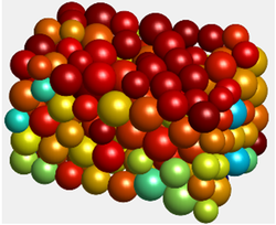
The basic model of the MatDEM code is a series of 3D close-packed elastic particles as shown in Figure 1a, and these particles interact through the spring forces (Figure 1b).
| ||||
| Figure 1. The contact model of particles in MatDEM |
The normal force and the normal relative displacement between two adjacent particles are simulated by a normal spring:
|
|
(1) |
where is the stiffness of the normal spring, and is the breaking displacement. Initially, the particles are interconnected with their adjacent particles and subjected to tensile or compressive spring forces as Eq. (1a). In case of between the particle pair exceeding , the spring breaks and the tensile force ceases to exist between them (Eq. (1b)). However, the compressive force may act between them when they return to a compressive status (Eq. (1c)). It is noticed that the tensile force is positive, and the compressive force is negative in Eq. (1).
The shear force and the tangential relative displacement between two particles are simulated by a tangential spring:
|
|
(2) |
where is the stiffness of the tangential spring. The tangential spring also has a fracture criterion based on the Mohr-Coulomb yield criterion:
|
|
(3) |
where is the inter-particle shear resistance, is the initial inter-particle shear resistance when no normal force exists, and is the inter-particle coefficient of friction. When the tangential force exceeds in Eq. (3a), the tangential spring will break, whereupon the shear force is limited to be less than or equal to the inter-particle shear resistance of the broken spring. If the tangential spring is broken and the magnitude of external shear force exceeds the limit in Eq. (3b), two particles begin slipping, and the slipping friction between them is in Eq. (3b).
2.2 Energy system of the MatDEM modeling
The MatDEM modeling follows the law of energy conversation and Newton’s law of motion. The energies of a model fall into two categories, mechanical energy and heat. A brief introduction of their compositions is given as follows.
(1) The mechanical energy in the system consists of elastic potential energy, gravitational potential energy and kinetic energy. The elastic potential energy is the sum of the strain energy of normal and tangential springs between particles:
|
|
(4) |
The gravitational potential energy of a particle is:
|
|
(5) |
where is the particle mass, denotes the gravity acceleration, and represents the height above the reference level. The kinetic energy of a particle is computed as:
|
|
(6) |
in which is the scalar of particle velocity.
(2) The heat in the system comes from the viscous damping, the spring breaking and the friction. Damping is used in the MatDEM to weaken the elastic wave energy of the model and dissipate the kinetic energy in the system. The damping force is given by
|
|
(7) |
where is the damping coefficient and is the vector of particle velocity. Because the time step of the simulation is very small, the particle velocity is assumed to be constant in a step. Viscous heat generated by viscous damping is calculated by
|
|
(8) |
in which denotes the particle displacement in the current time step.
When an intact spring breaks, the spring force reduces, and the elastic potential energy of the inter-particle normal spring and/or tangential spring will dissipate into heat. Thus, breaking heat is equal to the reduction of the elastic potential energy . The calculation of breaking heat is based on the status of the inter-particle normal force. If the inter-particle normal force is tensile, both the normal and tangential spring forces will reduce to zero, and thus the breaking heat is the sum of elastic potential energy of both normal and tangential springs:
|
|
(9) |
If the normal force is compressive, the normal spring force will not be changed, and the tangential spring force reduced from in Eq. (3a) to in Eq. (3b). The breaking heat is the reduction of the elastic potential energy of the tangential spring, which can be calculated by
|
|
(10) |
Friction heat generated during the sliding process is defined as the product of the average sliding friction and the effective sliding distance:
|
|
(11) |
in which and are the sliding friction forces at respectively the beginning and the end of the current time step, and denotes the effective sliding distance. More details about Eq. (11) can be found in [39].
The total energy of a MatDEM model is the sum of all mechanical energy and heat:
|
|
(12) |
where represents the sum of viscous heat , breaking heat and friction heat :
|
|
(13) |
Based on the law of energy conversation, the total energy of an isolated system is constant. If the system deforms under external force, the increment of the total energy must be equal to the work done by the external force.
3. A BP neural network-based micro particle parameters calibration
3.1 The structure of the BP neural network to predict the shear strength
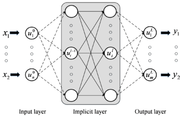
In this study, the BP neural network is used to establish the relationship between the shear strength and micro parameters for MatDEM modeling. BP neural network is a multilayer feed-forward neural network which consists of an input layer, implicit layer and output layer as shown in Figure 2 .
| |
| Figure 2. Typical structure of BP neural network |
When the value of neurons in the input layer is given, neurons in the implicit layer and the output layer are calculated according to the following forward propagation:
|
|
(14) |
where is the number of layers in the implicit layer, denotes the -th neuron in the -th layer, is the activation function, is the number of neurons in the -th layer, is the weight and is the deviation. The training of BP neural network indicates constantly adjusting the weights and deviations to minimize the differences between the output value and the true value.
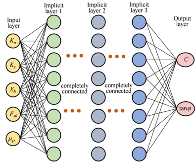
The structure of the BP neural network prediction model for the shear strength is plotted in Figure 3. The micro parameters are placed in the input layer and the shear strengths are placed in the output layer. It is noticed that only the micro parameters in terms of the particle contact model is involved in the BP neural network. Although some other micro parameters, e.g. the particle radius and the particle density, and the particle packing pattern have been verified to influence the macro mechanical properties of geotechnical materials in the numerical model [31], their effect is ignored in this study. The reason is that the particle radius and the particle density will be constant when the numerical model of the slope has been established, and all particles are prescribed to be close-packed in MatDEM.
| |
| Figure 3. BP neural network prediction model for the shear strength |
Considering that an ultimate aim of this study is to acquire the micro parameters corresponding to the original and reduced shear strength, the established BP neural network seems unfavorable. The reasons are explained as follows. If placing the micro parameters in the output layer and the shear strengths in the input layer, the output layer have more neurons than the input layer, which forms an underdetermined mathematical problem. In this situation, the BP neural network is possible to result in a result of low precision. For example, to calibrate micro particle parameters for Particle Flow Code (PFC) modeling, a BP neural network was built by placing three macro geotechnical mechanical parameters in the input layer and four micro parameters in the output layer [35]. Although the BP neural network database consists of four hundred samples, results of some testing samples were still unsatisfactory. Thus, the micro parameters and the shear strengths are placed in the input layer and the output layer respectively, to promise the validity of the BP neural network. Base on the BP neural network predict model of the shear strength, a calibration of the micro particle parameters will be developed similar to the work in [34].
3.2 Virtual 3D direct shear tests to measure the shear strength
The direct shear test and the triaxial compression test are two commonly used tests to measure the shear strength of geotechnical materials in laboratory, and their virtual counterparts have been established in DEM simulation by researchers [30,44]. Under the same micro parameter conditions, the two virtual tests are possible to result in different values of the shear strength [44]. Considering that the shear strength of geotechnical materials in the latter case study is obtained by using direct shear test, virtual 3D direct shear test is used to measure the shear strength in this study.
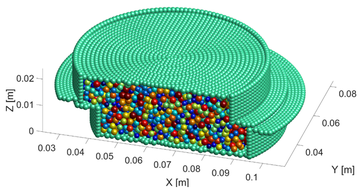
As shows in Figure 4, the virtual 3D direct shear test model consists of two parts, the specimen and the shear box. The specimen is composed of 7636 spherical particles, whose radiuses vary from 0.83 mm to 1.20 mm. The radius of the specimen is 30 mm and the height is 20 mm. The shear box consists of 7374 walls. To simulate the shearing process, the imposed boundary conditions are the horizontal velocity of the lower box and the normal pressure on the top wall. By prescribing the horizontal displacement of the lower box in each time step to be 0.05 mm, the shear stress was recorded until the specimen was finally damaged.
|
| Figure 4. Virtual 3D direct shear test model for measuring the shear strength of particle aggregate |
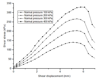
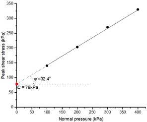
Given the micro particle parameters as N/mm, N/mm, m, Pa and , four normal pressures, 100 kPa, 200kPa, 300kPa and 400 kPa, are applied on the top wall to perform the virtual 3D direct shear test. The shear stress−shear displacement curves under the four normal pressures are plotted in Figure 5a. The trend of the four curves is consistent with each other. The increasing of the imposed normal pressures induces a higher peak value of the shear stress, and the shear displacement where the shear stress reaches its peak value increases slightly, which is similar to the result of the previous virtual direct shear test [44]. The Coulomb formula
|
|
(15) |
is employed to determine the shear strength of the particle aggregate as shown in Figure 5b. Finally, the friction angle is 32.4°, and the cohesion is 76 kPa.
| ||||
| Figure 5. Virtual 3D direct shear test model for the shear strength measurement |
3.3 A correction calibration of micro particle parameters based on the BP neural network
Based on the previous studies on the influence of the micro particle parameters in MatDEM on the mechanical properties of the particle aggregate [39], four levels are considered for and , and three levels are considered for , and when establishing the BP neural network database. Table 1 lists the level values of micro particle parameters. By using the full orthogonal combination, 432 combinations of micro particle parameters are generated. And then, the virtual 3D direct shear test is executed to obtain their corresponding shear strengths. Finally, the BP neural network database is composed by 432 groups of micro particle parameters and the corresponding shear strengths.
| (N/m) | (N/m) | (Pa) | (m) | |
|---|---|---|---|---|
| , , | , , | , , , | , , |
The training of the BP neural network actually successfully establishes the mapping relationship between the micro particle parameters in the input layer and the shear strengths in the output layer, which can be denoted as the following formula.
|
|
(16) |
Assuming that the shear strengths (outputs) are continuous in the micro particle parameter space, the micro particle parameters (inputs) corresponding to the target shear strengths could be resolved similarly to the resolution of the nonlinear equations, because the gradient at any given input could be computed in the BP neural network. In the first place, an objective function is defined as
|
|
(17) |
where and are the target cohesion and the target friction angle, respectively. And then, the gradient descent method is used to adjust the inputs until the objective function have a value smaller than the prescribed threshold value. For a simplicity expression, the input (, , , , ) is denoted by , the output (, ) is denoted by , and thus Eq. (16) can be written as . The resolution process is explained as follows:
(1) Determine the initial exploration input by using the K-means clustering analysis [45]. K-means clustering is a vector quantization method originally from signal processing and can partition observations into clusters where each observation belongs to the cluster with the nearest mean. The samples in the neural network database are partitioned into clusters by using K-means clustering analysis. K is takens as 15 in this study. Distances between the cluster centers and the target are computed by Eq. (17), and the nearest cluster center is selected as .
(2) Calculate the response outputs for the exploration point of at step , and then invoke the objective function. When the objective function has a value smaller than the threshold value, the resolution is terminated and takes the value of . If not, continue to perform step (3).
(3) Calculate the gradient of the objective function at , and update along the descent direction of the objective function. The formulation to update is
|
|
(18) |
in which is the increment used to update and is the step length. is obtained by multiplying the negative gradient of the objective function by . On account of the nonlinearity of forward propagation rule, is introduced for performing a step search approximation along the error gradient descent direction.
(4) Let and return to step (2).
Forward propagation of the established BP neural network can be regarded as a substitution of the virtual 3D direct shear test. The samples in the neural network database are always finite, which indicates that the substitution is certain to be approximate. Therefore, the inputs obtained from the mathematical resolution may have a low accuracy. An additional step called as “verifying test” is used to determine whether the inputs are acceptable. The verifying test performs virtual 3D direct shear test by using the inputs obtained from the mathematical resolution, and calculates the error between the resulted shear strength and the target by using Eq. (17). If the objective function has a value smaller than the threshold value, the inputs are acceptable. Otherwise, a correction should be introduced for obtain a more reasonable input.
The failure of the verifying test indicates that the current BP neural network is still not accurate enough to obtain a fine mathematical resolution. A feasible strategy to improve the precision of BP neural network is adding some new samples to the database. Although the current BP neural network is not accurate enough, it provides a rough search direction for the resolution and the inputs resulted by the last round of the mathematical resolution must be a bit closer to the optimal solution than the initial inputs. Considering that, a new sample consisting of the resulted inputs in the last round and the corresponding shear strength is added to the database, and then the neural network is retrained. After the retraining of the BP neural network, the mapping relationship in Eq. (16) has been replaced by a new relationship. Then, the mathematical resolution is executed again by selecting the resulted inputs in the last round as the initial exploration input, and the verifying test is performed again. The “mathematical resolution−verifying test−neural network correction” flow is repeated till the objective function has a value smaller than the threshold value in verifying test. The entire flow of the correction method to calibrate the micro particle parameters is plotted in Figure 6 .
| |
| Figure 6. The entire flow of the correction method to calibrate the micro particle parameters |
3.5 Validity of the proposed correction calibration
To verify the validity of the proposed calibration method, four different target shear strengths are given, and the optimal micro particle parameters are searched by prescribing the threshold value as for Eq. (17). After three or four rounds of mathematical resolution, the resulted micro particle parameters passed the verifying test. Table 2 lists the micro parameters provided by the mathematical resolution and the shear strengths provided by the verifying test in each round.
| Target shear strength | Round | (N/m) | (N/m) | (m) | (Pa) | (kPa) | ||
|---|---|---|---|---|---|---|---|---|
| kPa |
1 | |||||||
| kPa |
||||||||
| kPa |
||||||||
| kPa |
||||||||
Results in Table 2 shows that in Eq. (17) decreases whith the mathematical resolution round increasing, which implies that the target shear strengths are approximated gradually. Taking the case =30.0 kPa, as an example, the relative errors of the resulted shear strengths are respectively 27.7% and 63.5% for the cohesion and the friction coefficient in the first round, by using the target shear strengths as the reference. In the second round, they decrease to 5.3% and 18.1% for the cohesion and the friction coefficient, respectively. Ultimately, they decrease to 0.7% and 0.2% in the fourth round for the cohesion and the friction coefficient, respectively. Thus, the proposed method has the ability to obtain the micro particle parameters that well reflects the shear strengths of particle assembly.
When performing the slope stability analysis by applying SRM in MatDEM, the shear strengths of the geological material in the MatDEM modeling are constantly adjusted. Once a new value of the shear strengths is given, a new combination of micro particle parameters is to be searched. At the moment, the established neural network database will provide a new initial exploration input by using the K-means clustering analysis, and then the proposed method is performed to obtain the micro particle parameters.
4. An energy criterion to evaluate the slope stability
As mentioned in Section 2.2, the MatDEM modeling follows the law of energy conversation and Newton’s law of motion. When slope instability happens, the displacements of soil and rock will induce the conversion between various kinds of energies. Consequently, the energy conversion of an instable slope in MatDEM must be different with that of a stable slope. In this section, a simple 2D slope is taken as an example to investigate the energy conversion difference between the stable and instable slope. And then, an energy criterion is established to evaluate the slope stability.
4.1 Investigation on the energy conversion difference between the stable and instable slope
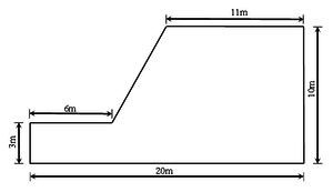
As shows in Figure 7, the slope is 7 m height and the ratio of slope is 7: 3. And, the slope is assumed to be homogeneous and composed by one kind of geotechnical material for simplicity. The MatDEM model of the slope contains 6305 particles. The radius of particles varies from 0.064 m to 0.096 m. The density is taken as 2.04×10³ kg/m3, and the gravity acceleration m/s2. All particles at the left, right and bottom boundaries are fixed as the boundary conditions of the model.
|
| Figure 7. A simple homogeneous slope 2D model |
In the numerical simulation of the slope model, three groups of micro particle parameters listed in Table 3 are selected, which are denoted as Case 1, 2 and 3 respectively. Considering that the chief purpose here is to reveal the energy conversion difference between the stable and instable slope, the shear strengths are not measured for the three groups of micro particle parameters by using the virtual numerical test.
| Parameter | (N/m) | (N/m) | (m) | (Pa) | |
|---|---|---|---|---|---|
| Case 1 | |||||
| Case 2 | |||||
| Case 3 |
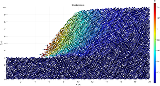
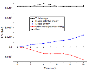
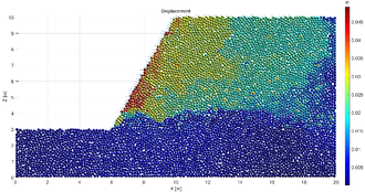
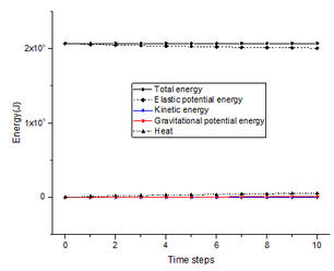
After 10 time steps of the computation, the slope is verified to be instable in Case 1 but stable in Case 2 and 3. It is noticed that one time step in MatDEM consists of a number of sub-time steps, and the value of a sub-time step is self-determined by the software. In the computation of the slope model, one time step is composed of 63 sub-time steps, and a sub-time step takes 0.0001, 0.00015 and 0.0002 for Case 1, Case 2 and Case 3, respectively. The displacement cloud charts are plotted in Figure 8a and Figure 9a for Case 1 and Case 2, respectively. The displacement cloud chart of Case 3 is not provided because the displacement difference between Case 2 and Case 3 is not noticeable. Figure 8b and Figure 9b illustrate the variations of the total energy, elastic potential energy, kinetic energy, gravitational potential energy and heat with the time steps for Case 1 and Case 2, respectively. Some interesting phenomena are observed in the energy-time steps curves, and a further investigation is valuable for the establishment of an energy criterion to evaluate the slope stability.
| ||||
| Figure 8. Displacements and the energy conversion for the slope in Case 1 |
| ||||
| Figure 9. Displacements and the energy conversion for the slope in Case 2 |
Firstly, the conclusion that MatDEM follows the law of energy conversation is confirmed again by the energy-time steps curves. For both two cases, the total energies are almost constant during the computation, no matter whether the slope is stable or not. However, the total energy of Case 2 has a larger value than that of Case 1, which can be explained as follows. In the MatDEM modeling, the gravitational potential energy is evaluated by the relative vertical displacement of particles. It is initialized to be zero for a particle, and becomes negative when the particle falls while positive when the particle rises. The kinetic energy is zero for a particle unless the motion of the particle happens. The heat induced by the viscous damping, the spring breaking and the friction is zero in the initial state. Therefore, the total energy should be equal to the elastic potential energy initially. Since the elastic potential energy is computed as Eq. (4), and dominate the value of the elastic potential energy. Because the values of and in Case 2 is greater than that in Case 1, the total energy of Case 2 has a larger value than that of Case 1.
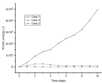
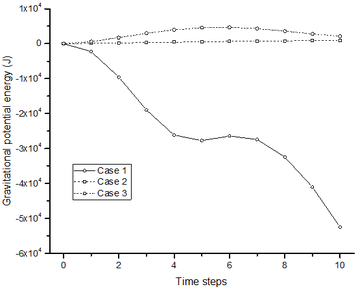
Secondly, the variations of the kinetic energy and the gravitational potential energy in Figure 8b and Figure 9b are apparently different. With the time step increasing, the kinetic energy increases but the gravitational potential energy decreases in Figure 8b. But, the gravitational potential energy and the kinetic energy are nearly constant in Figure 9b. Figure 10 plots the variations of the kinetic energy and the gravitational potential energy with time steps for all three cases.
| ||||
| Figure 10. Variations of the kinetic energy and the gravitational potential energy with time steps for all three cases |
For Case 3, the kinetic energy is observed, and the gravitational potential energy is positive. That may be caused by the slope deformation. The kinetic energy and the gravitational potential energy caused by the deformation can be easily distinguished from that caused by the failure. Above all, the magnitude of the energy induced by the deformation is tiny compared to that induced by the failure. For Case 3, the kinetic energy and the gravitational potential energy have peak values of 2800 J and 4700 J, respectively. For Case 2, they have peak values of 116 J and 945 J, respectively. Next, when the two energies are caused by deformation, their variations show the convergent trend. But, when the two energies are induced by the failure, their variations show the divergent trend. Since the clear difference in the variation of the kinetic energy and the gravitational potential energy can be observed between a stable slope and an instable slope, they have the potential to be used in the evaluation of the slope stability.
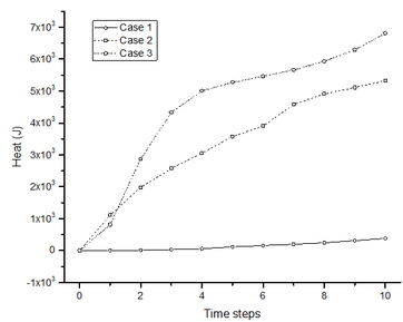
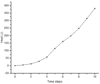
Finally, the heat is investigated. The variations of heat are illegible in Figure 8b and Figure 9b because the magnitude of heat is too small. Figure 11a plots the variations of the heat with time steps for all three cases. Obviously, the heats in Case 2 and Case 3 are much greater than that in Case 1. But it is incorrect to have a conclusion that the heat in a stable MatDEM slope model is more than that in an instable MatDEM slope model. The heat in the system is composed of the contributions of the viscous damping, the spring breaking and the friction force, in which the latter two sources are calculated based on the micro particle parameters. In Figure 11a, the heat curve for Case 1 is situated in the lowest position, which maybe resulted by the micro particle parameters in Table 3. Thus, the magnitude of the heat is unreasonable to be chosen as a reference in the slope stability assessment. But, the shapes of the three heat curves are quite different. For a better demonstration, the heat curve is repainted for Case 1 in Figure 11b. The heat curves of Case 2 and Case 3 are roughly convex, but the heat curve of Case 1 is concave. If the slope is stable, the position change of the particles induced by the deformation will stop rapidly, which promises the heat to be stable after several time steps. If the slope is sliding, the positions of the particles are still continuously changed, which results in the on-going increasing of the heat. Therefore, the shape of the heat curve may be effective in the evaluation of the slope stability.
| ||||
| Figure 11. Variations of the heat with time steps [68] |
4.2 A criterion based on the kinetic energy of the MatDEM model
As mentioned in the Section 4.1, the variation of the kinetic energy and the gravitational potential energy and the shape of the heat curve are verified to be different between a stable slope and an instable slope when performing the simulation by MatDEM. Their validities are compared in this section from a view of practical application.
When performing the slope stability analysis by using SRM in MatDEM, the micro parameters of the particles will be modified according to the reduction factor. Both the gravitational potential energy and the kinetic energy are independent of the micro particle parameters. However, the heat is calculated based on the micro particle parameters. When the energy variations resulted by using different micro particle parameters are collected together, it is more suitable to compare the results of the gravitational potential energy and the kinetic energy than that of the heat. Additionally, the number of the time steps has a great influence on the reliability of the conclusion if estimating the stable state of a slope by using the shape of the heat curves. As shows in Figure 11a, the overall trend of the heat curve is convergent for Case 2, while a slight turning happens at the sixth time step. A large number of time steps seem to be feasible to overcome the effect of the local abnormality, but it will cause another issue. In fact, the heat curve must be convergent ultimately no matter whether the slope is stable or not. In case of an instable slope, the position of the particles will be relocated finally when the sliding is terminated, and thus the heat will be also stable. Therefore, an incorrect conclusion may be drawn based on the shape of the heat curve when the number of time steps is inappropriate. In short, the gravitational potential energy and the kinetic energy are more suitable to be compared than the heat when estimating the stable state of a slope.
There is an essential association between the gravitational potential energy and the kinetic energy. The motion of the particles results in the change of their positions, so the kinetic energy always emerges before the gravitational potential energy in MatDEM. This deduction can be verified by the variations of the kinetic energy and the gravitational potential energy for Case 3. As shown in Figure 10 , for Case 3 it is the fourth time step that the kinetic energy begins to decrease, while it is the seventh time step that the gravitational potential energy begins to decrease. This phenomenon indicates that the convergence of the kinetic energy should be earlier than that of the gravitational potential energy for a stable slope. Moreover, the variation of the gravitational potential energy is noticed to be small when the time step ranges from four to seven for Case 1. The reason is that the motion of the particles in the model maybe temporarily dominated by the horizontal motion during the failure, but only the vertical motion of the particles induces the variation of the gravitational potential energy. Thus, the gravitational potential energy may have a more complicated curve than the kinetic energy. Based on the above analysis, the kinetic energy is taken as the main reference to estimate the stable state of a slope.
When performing the slope stability analysis by using SRM in MatDEM, the variations of the kinetic energy are collected under different reduction factors. Then, the variation tendencies and the magnitude of the kinetic energies are compared. The abrupt in the variation tendencies and the magnitude is considered as a sign for the emergence of the critical point, and the safe factor of the slope is determined finally. At this point, a criterion has been proposed to evaluate the slope stability based on the kinetic energy.
5. Case study: Baijiabao landslide
5.1 Geological background
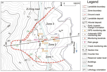
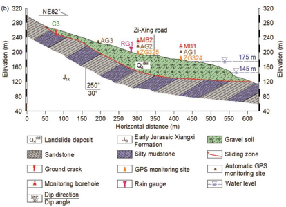
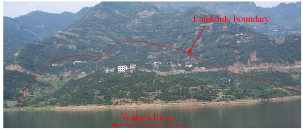
Baijiabao landslide is situated in Guizhou village of Zigui County, Hubei Province of China on the right bank of the Xiangxi River (30o58′59.9′′N, 110o45′33.4′′E). A photograph of the landslide that was taken from the opposite bank of the Xiangxi River is shown in Figure 12. The elevation of the landslide ranges from 125 m to 265 m above MSL, and the slope of the landslide ranges from 10o to 20o. The upper boundary of the landslide is defined by the interface between the bedrock and the soil. The left and right boundaries are defined by two natural gullies that contain many surface cracks. The toe of the landslide varies in elevation between 125 m to 135 m. The primary sliding direction of Baijiabao landslide varies between 75o and 85o (SW-NE). This landslide is 550 m long and 400 m wide, covers an area of 20 ha, and has an estimated volume of nearly 1 million m3. The landslide mass is primarily composed of loose Quaternary deposits. Its sliding zone is mainly silty clay. And the underlying bedrock contains quartz sandstone and argillaceous siltstone of the Early Jurassic Xiangxi Formation, which dips into the hill at an angle of 30o to 40o (Figure 13).
|
| Figure 12. A photograph of Baijiabao landslide, taken from the opposite bank of the Xiangxi River |
| ||||
| Figure 13. Geological background of Baijiabao landslide [46] |
Baijiabao landslide poses significant threats to public safety. The Zi-Xing road crosses the central part of the landslide mass as Figure 13a shows. Before Three Gorges Reservoir (TGR) impoundment, 165 residents lived in the landslide area, while only 20 residents live there today. The deformation rate of the landslide was observed to increase significantly after TGR impoundment. Monitoring system installed in October 2006 consists of four GPS monitoring sites, which are noted as ZG323, ZG324, ZG325 and ZG326 in Figure 13a. The detailed deformation history of Baijiabao landslide can be referred to the related literatures [46-48].
5.2 Landslide model in the MatDEM modeling
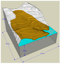
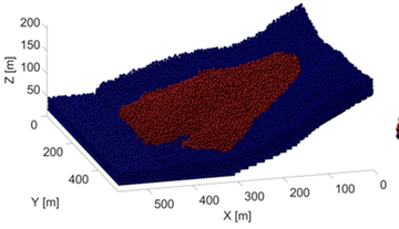
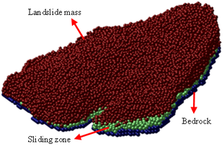
This subsection describes the establishment of the 3D MatDEM model for the stability analysis of Baijiabao landslide. Firstly, the geomorphy of the landslide is simulated by using ArcGIS software based on the contour line measured in 2006 (Figure 14a). Then, a 3D model of Baijiabao landslide is built in MatDEM. The model is 564 m long, 497 m wide and 186 m height, covering the whole landslide mass (Figure 14b). Next, geotechnical materials are allocated according to the engineering geologic investigation data. The sliding zone in the model (Figure 14c) is positioned by using the interpolation of locations where the sliding zone is encountered in the drilling exploration. The landslide mass has a thickness varying between 20 m to 30 m in the front area, and has a thickness varying between 10 m to 40 m in the trailing area.
| ||||||
| Figure 14. 3D MatDEM model for the stability analysis of Baijiabao landslide |
Finally, the 3D MatDEM model of Baijiabao landslide is composed by 1,207,985 particles, in which the landslide mass and the sliding zone are represented by 733,104 removable particles, and the bedrock is represented by 474,881 fixed particles. The radius of particles varies between 0.55 m and 0.83 m. In Figure 14c, the landslide mass, the sliding zone and the bedrock are presented as brown particles, green particles and blue particles, respectively.
5.3 Mechanical parameters and micro particle parameters
According to the report of engineering geological exploration, the unit weight and shear strengths are listed in Table 4 for the geotechnical materials in the landslide mass, the sliding zone and the bedrock, respectively. All parameters are measured in the native state, and taken their statistical mean value. It is noticed that the stability of Baijiabao landslide is actually affected by the rainfall and the reservoir water fluctuation. In view that the main purpose of this study is to improve the ability of MatDEM in 3D slope stability evaluation, the rainfall and the reservoir water fluctuation are ignored temporarily.
| Region | Unit weight (kN/m3) | (kPa) | (o) |
|---|---|---|---|
| Landslide mass | 18.0 | 17.1 | 20.2 |
| Sliding zone | 20.5 | 24.6 | 15.2 |
| Bedrock | 26.0 | 1,200 | 32.1 |
Using the BP neural network-based calibration method established in Section 3, micro parameters of particles representing various geotechnical materials are obtained and listed in Table 5. Because the particles have a much larger radius than the particles used in Section 3, the size of the virtual 3D direct shear test model is adjusted. Previous studies [21,49] verified the effect of the particle size on the macro properties in DEM modeling, and declared that the ratio / is a critical variable to be carefully selected when performing virtual strength test. Here is the size of the strength test model, and denotes the average radius of particles. According to Su’s suggestion [49], / should be more than 200 to avoid the effect of the particle size on the macro properties of the particle assembly in DEM. Finally, the specimen to be used in virtual 3D direct shear test has a radius of 21 m and a height of 14 m.
| Region | (N/m) | (N/m) | (m) | (Pa) | (kPa) | (o) | |
|---|---|---|---|---|---|---|---|
| Landslide mass | |||||||
| Sliding zone | |||||||
| Bedrock |
With respect to the bedrock, the micro particle parameters in Table 5 resulted in the shear strengths different to the actual shear strengths in Table 4. The reason is that it is hard to represent the three geotechnical materials by using micro parameters of the same order of magnitude. The cohesion of the bedrock is nearly 100 times that of the landslide mass and the sliding zone. Because all the particles representing the bedrock are fixed in the model, the difference between the cohesion of the bedrock in Table 4 and that in Table 5 will have little influence on the computation. Moreover, to reduce the workload, the micro particle parameters of the bedrock will not be changed when the stability of the landslide is evaluated by using SRM.
5.4 Computational results
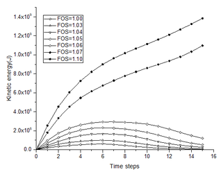
As concluded in Section 4, the abrupt in the variation tendencies and the magnitude of the kinetic energy can be utilized to determine the FOS when estimating the slope stability by using SRM in MatDEM. Under different reduction factors, the variations of the kinetic energy with time steps are recorded for the landslide model and plotted in Figure 15. The kinetic energy curve resulted by a greater reduction factor always has a higher situation in Figure 15. But, if the reduction factor is less than 1.06, the difference in the magnitude of the kinetic energy between different reduction factors is relatively small at each time step. When the reduction factor is increasing from 1.06 to 1.07, the magnitude difference has a dramatically increasing. Meanwhile, the kinetic energy curves present a convergent trend when the reduction factor is less than 1.06, but present a divergent trend when the reduction factor arrives at 1.07. Thus, the FOS of Baijiabao landslide is considered as 1.06.
|
| Figure 15. Variation of kinetic energy with time steps under different reduction factors |
By using the proposed BP neural network-based calibration method, the micro particle parameters are constantly adjusted during the computation. Table 6 lists the micro particle parameters and the shear strengths under different reduction factors.
| Region | FOS | (N/m) | (N/m) | (m) | (Pa) | (kPa) | (o) | |
|---|---|---|---|---|---|---|---|---|
| Landslide mass | ||||||||
| Sliding zone | ||||||||
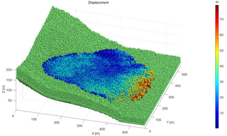
Figure 16 illustrates the final displacement of Baijiabao landslide model when the reduction factor is taken as 1.06. Some particles in the front area of the model have the displacements of nearly 60 m, and most particles have the displacements less than 10 m. Thus, the FOS determined by the abrupt in the variation tendencies and the kinetic energy magnitude in fact reveals the landslide stability at the global level. The displacements when the landslide is close to its limit equilibrium state may be valuable in the landslide failure prediction. The field data [46] verified that at the monitoring period from January 2007 to December 2019, the ZG326 site (Figure 13a) in the middle area of Baijiabao landslide recorded the max cumulative displacement of 1.8 m. Its displacements are still observed when the reservoir water level changes and the rainfall happen, while Baijiabao landslide hasn’t slipped entirely till now. Therefore, the surface movements before its failure are uncertain. In views that this study aims to establish a micro particle parameter calibration method and a criterion for the application of SRM in MatDEM to analysis 3D slope stability, the influence of the reservoir water and the rainfall on the stability of Baijiabao landslide is left out of consideration. Hence, the displacements in the limit equilibrium state obtained in this study are not suitable for the failure prediction for Baijiabao landslide.
|
| Figure 16. The displacement of Baijiabao landslide model with the reduction factor 1.06 |
6. Conclusions
By taking MatDEM as an example, a calibration method based on BP neural network is proposed to acquire the micro particle parameters corresponding to the given shear strengths in this paper, and an energy criterion is proposed for determining the FOS of the slope when applying SRM in DEM. And the proposed enhancements are applied in the 3D stability analysis of Baijiabao landslide. The following conclusions can be made:
(1) BP neural network can well represent the complicated relationship between the micro particle parameters and the shear strengths of the particle aggregate in MatDEM. And the proposed BP neural network-based micro particle parameters calibration method is applicable to provide the micro particle parameters when the shear strength is constantly reduced.
(2) The variations of the kinetic energy, the gravitational potential energy and the heat are noticed to be quite different between the stable and instable slope. However, the abrupt in the variation tendency and the magnitude of the kinetic energy is more suitable for determining the FOS of the slope.
(3) When determining the FOS by using the kinetic energy criterion, the displacements of particles in the slope model are permitted, so the FOS actually reveals the slope stability at the global level.
Acknowledgments
The work is supported by the Open Research Programme of the Hubei Key Laboratory of Disaster Prevention and Mitigation (China Three Gorges University) (no. 2022KJZ07), the Open Research Fund of Key Laboratory of Geological Hazards on Three Gorges Reservoir Area of Ministry of Education (2020KDZ10), National Natural Science Funds (Project No. 52079070), and the Open Research Fund of State Key Laboratory of Simulation and Regulation of Water Cycle in River Basin (China Institute of Water Resources and Hydropower Research), Grant NO:IWHR-SKL-202020.
References
[1] Sun G., Jiang W., Cheng S., Zheng H. Optimization model for determining safety factor and thrust line in landslide assessments. International Journal of Geomechanics, 17(4):04016091, 2017.
[2] Deng D.P., Li L., Zhao L.H. LEM for stability analysis of 3D slopes with general-shaped slip surfaces. International Journal of Geomechanics, 17(10):06017017, 2017.
[3] Firincioglu B.S., Ercanoglu M. Insights and perspectives into the limit equilibrium method from 2D and 3D analyses. Engineering Geology, 281:105968, 2021.
[4] Lv Q., Liu Y., Yang Q. Stability analysis of earthquake-induced rock slope based on back analysis of shear strength parameters of rock mass. Engineering Geology, 228:39-49, 2017.
[5] Zheng H., Sun G., Liu D. A practical procedure for searching critical slip surfaces of slopes based on the strength reduction technique. Computers and Geotechnics, 36(1-2):1-5, 2009.
[6] Espada M., Muralha J., Lemos J.V., Jiang Q., Feng X.-T., Fan Q., Fan Y. Safety analysis of the left bank excavation slopes of Baihetan arch dam foundation using a discrete element model. Rock Mechanics and Rock Engineering, 51(8):2597-2615, 2018.
[7] Lu, Y., Tan, Y. and Li, X. Stability analyses on slopes of clay-rock mixtures using discrete element method. Engineering Geology, 244: 116-124, 2018.
[8] Nie Z., Zhang Z., Zheng H., Lin S. Stability analysis of landslides using BEM and variational inequality based contact model. Computers and Geotechnics, 123:103575, 2020.
[9] Sun G., Lin S., Zheng H., Tan Y., Sui T. The virtual element method strength reduction technique for the stability analysis of stony soil slopes. Computers and Geotechnics, 119:103349, 2020.
[10] Xu D., Wu A., Yang Y., Lu B., Liu F., Zheng H. A new contact potential based three-dimensional discontinuous deformation analysis method. International Journal of Rock Mechanics and Mining Sciences, 127:104206, 2020.
[11] Yang Y., Xia Y., Zheng H., Liu Z. Investigation of rock slope stability using a 3D nonlinear strength-reduction numerical manifold method. Engineering Geology, 292:106285, 2021.
[12] Wang B., Vardon P.J., Hicks M.A. Rainfall-induced slope collapse with coupled material point method. Engineering Geology, 239:1-12, 2018.
[13] Bui H.H., Fukagawa R., Sako K., Wells J.C. Slope stability analysis and discontinuous slope failure simulation by elasto-plastic smoothed particle hydrodynamics (SPH). Géotechnique, 61(7):565-574, 2011.
[14] He L., Tian Q., Zhao Z., Zhao X., Zhang Q., Zhao J. Rock Slope stability and stabilization analysis using the coupled DDA and FEM method: NDDA approach. International Journal of Geomechanics, 18(6):04018044, 2018.
[15] Sun L., Liu Q., Abdelaziz A., Tang X., Grasselli G. Simulating the entire progressive failure process of rock slopes using the combined finite-discrete element method. Computers and Geotechnics, 141:104557, 2022.
[16] Bao Y., Sun X., Chen J., Zhang W., Han X., Zhan J. Stability assessment and dynamic analysis of a large iron mine waste dump in Panzhihua, Sichuan, China. Environmental Earth Sciences, 78(2):48, 2019.
[17] Jiang M., Niu M., Zhang F., Wang H., Liao Z. Instability analysis of jointed rock slope subject to rainfall using DEM strength reduction technique. European Journal of Environmental and Civil Engineering, 26(10):4664-4686, 2021.
[18] Shi C., Yang B., Zhang Y., Yang J. Application of discrete-element numerical simulation for calculating the stability of dangerous rock mass: A case study. International Journal of Geomechanics, 20(12):04020231, 2020.
[19] Zienkiewicz O.C., Humpheson C., Lewis R.W. Associated and non-associated visco-plasticity and plasticity in soil mechanics. Geotechnique, 25(4):671-689, 1975.
[20] Griffiths D.V., Lane P.A. Slope stability analysis by finite elements. Géotechnique, 49(3):387-403, 1999.
[21] Yang B., Jiao Y., Lei S. A study on the effects of microparameters on macroproperties for specimens created by bonded particles. Engineering Computations, 23(6):607-631, 2006.
[22] Zhou Z.H., Wang H.N., Jiang M.J. Macro- and micro-mechanical relationship of the anisotropic behaviour of a bonded ellipsoidal particle assembly in the elastic stage. Acta Geotechnica, 16(12):3899-3921, 2021.
[23] Cheng Y., Wong L.N.Y. A study on mechanical properties and fracturing behavior of Carrara marble with the flat‐jointed model. International Journal for Numerical and Analytical Methods in Geomechanics, 44(6):803-822, 2020.
[24] Liu C., Pollard D.D., Shi B. Analytical solutions and numerical tests of elastic and failure behaviors of close-packed lattice for brittle rocks and crystals. Journal of Geophysical Research: Solid Earth, 118(1):71-82, 2013.
[25] Rackl M., Hanley K.J. A methodical calibration procedure for discrete element models. Powder Technology, 307:73-83, 2017.
[26] Hou J., Zhang M., Chen Q., Wang D., Javadi A., Zhang S. Failure-mode analysis of loose deposit slope in Ya’an-Kangding Expressway under seismic loading using particle flow code. Granular Matter, 21(1):8, 2019.
[27] Su H., Fu Z., Gao A., Wen Z. Numerical simulation of soil levee slope instability using particle-flow code method. Natural Hazards Review, 20(2):04019001, 2019.
[28] Xu G.J., Zhong K.Z., Fan J.W., Zhu Y.J., Zhang Y.Q. Stability analysis of cohesive soil embankment slope based on discrete element method. Journal of Central South University, 27(7):1981-1991, 2020.
[29] Wang M., Cao P. Calibrating the micromechanical parameters of the PFC2D (3D) models using the improved simulated annealing algorithm. Mathematical Problems in Engineering, 2017:6401835, 2017.
[30] Cheng H., Shuku T., Thoeni K., Yamamoto H. Probabilistic calibration of discrete element simulations using the sequential quasi-Monte Carlo filter. Granular Matter, 20(1):11, 2018.
[31] Do H.Q., Aragón A.M., Schott D.L. A calibration framework for discrete element model parameters using genetic algorithms. Advanced Powder Technology, 29(6):1393-1403, 2018.
[32] Benvenuti L., Kloss C., Pirker S. Identification of DEM simulation parameters by Artificial Neural Networks and bulk experiments. Powder Technology, 291:456-465, 2016.
[33] He P., Fan Y., Pan B., Zhu Y., Liu J., Zhu D. Calibration and verification of dynamic particle flow parameters by the back-propagation neural network based on the genetic algorithm: recycled polyurethane powder. Materials, 12(20):3350, 2019.
[34] Ye F., Wheeler C., Chen B., Hu J., Chen K., Chen W. Calibration and verification of DEM parameters for dynamic particle flow conditions using a backpropagation neural network. Advanced Powder Technology, 30(2):292-301, 2019.
[35] Zhou, Y., Wu S., Jiao J., Zhang X. Research on mesomechanical parameters of rock and soil mass based on BP neural network. Rock Soil Mech, 32(12):3821-3826, 2011.
[36] Wang H., Zhang B., Mei G., Xu N. A statistics-based discrete element modeling method coupled with the strength reduction method for the stability analysis of jointed rock slopes. Engineering Geology, 264:105247, 2020.
[37] Deluzarche R., Cambou B. Discrete numerical modelling of rockfill dams. International Journal for Numerical and Analytical Methods in Geomechanics, 30(11):1075-1096, 2006.
[38] Shen H., Abbas S.M. Rock slope reliability analysis based on distinct element method and random set theory. International Journal of Rock Mechanics and Mining Sciences, 61:15-22, 2013.
[39] Liu C., Xu Q., Shi B., Deng S., Zhu H. Mechanical properties and energy conversion of 3D close-packed lattice model for brittle rocks. Computers & Geosciences, 103:12-20, 2017.
[40] Liu Y., Zhang D., Wang G.-y., Liu C., Zhang Y. Discrete element method-based prediction of areas prone to buried hill-controlled earth fissures. Journal of Zhejiang University-SCIENCE A, 20(10):794-803, 2019.
[41] Luo H., Xing A., Jin K., Xu S., Zhuang Y. Discrete element modeling of the Nayong rock avalanche, Guizhou, China constrained by dynamic parameters from seismic signal inversion. Rock Mechanics and Rock Engineering, 54(4):1629-1645, 2021.
[42] Scaringi G., Fan X., Xu Q., Liu C., Ouyang C., Domènech G., Yang F., Dai L. Some considerations on the use of numerical methods to simulate past landslides and possible new failures: the case of the recent Xinmo landslide (Sichuan, China). Landslides, 15(7):1359-1375, 2018.
[43] Zhan Q., Wang S., Wang L., Guo F., Zhao D., Yan J. Analysis of failure models and deformation evolution process of geological hazards in Ganzhou city, China. Frontiers in Earth Science, 9:731447, 2021.
[44] Graziani A., Rossini C., Rotonda T. Characterization and DEM modeling of shear zones at a large dam foundation. International Journal of Geomechanics, 12(6):648-664, 2012.
[45] Peña J.M., Lozano J.A., Larrañaga P. An empirical comparison of four initialization methods for the K-Means algorithm. Pattern Recognition Letters, 20(10):1027-1040, 1999.
[46] Yao W.M., Li C.D., Guo Y.C., Criss R.E., Zuo Q.J., Zhan H.B. Short-term deformation characteristics, displacement prediction, and kinematic mechanism of Baijiabao landslide based on updated monitoring data. Bulletin of Engineering Geology and the Environment, 81(9):393, 2022.
[47] Xu S.L., Niu R.Q. Displacement prediction of Baijiabao landslide based on empirical mode decomposition and long short-term memory neural network in Three Gorges area, China. Computers & Geosciences, 111:87-96, 2018.
[48] Yao W.M., Li C.D., Zuo Q.J., Zhan H.B., Criss R.E. Spatiotemporal deformation characteristics and triggering factors of Baijiabao landslide in Three Gorges Reservoir region, China. Geomorphology, 343:34-47, 2019.
[49] Su, H., Yang J., Hu B., Gao X., Ma H. Study of particle size effect of rock model based on particle discrete element method. Rock and Soil Mechanics, 39(12):4642-4650, 2018.Document information
Published on 19/01/23
Accepted on 13/01/23
Submitted on 03/12/22
Volume 39, Issue 1, 2023
DOI: 10.23967/j.rimni.2023.01.003
Licence: CC BY-NC-SA license
Share this document
Keywords
claim authorship
Are you one of the authors of this document?
