Real options valuation with changing volatility

Summary

This paper aims at the valuation of real options with changing volatility. Volatility change is a typical feature of real investment projects, where the riskiness of cash flow generated by the project can change significantly during the project life span. In this paper, there is explained how the problem of changing volatility can be considered if binomial lattice and replication strategy is used for real option valuation. There are recombining and non-recombining lattice used and constant and increasing volatility are analysed and results compared. In situation when volatility is changing, two approaches overcoming this problem are employed and compared.

JEL classification

G11 ; G12 ; G13 ; G31

Keywords

Real options ; Valuation ; Risk-neutral ; Transition probabilities ; Binomial lattice ; Recombining ; Non-recombining ; Volatility

Introduction

Real options methodology is a relatively new approach for solution of a wide range of valuation and decision-making issues. Here, traditional methods and models used for financial option valuation are used for real assets valuation. Compared to the traditional passive valuation approaches (NPV, IRR, etc.), real option approach takes into consideration two important aspects: (a) riskiness of cash flow generated by the assets and (b) flexibility, i.e. capability of management to change past decision or to make new ones in already undertaken projects. These future possible decisions (depends on the future state of the world) are modelled as a formal call and put options, which have their value and can be exercised by companys management. Real asset value provided by the real option methodology application is given as a sum of two components: present value of directly measurable cash flows and flexibility value, which captures managerial possibilities (real options).

As mentioned, assets value and future managerial opportunities captured in real options are quantified by financial option valuation models. These models are based on some assumptions, which are sometimes difficult to keep due to the specific feature of real investments and real options captured in them (constant volatility, risk free rate, etc.). That is why it is necessary to adjust these models to specific conditions of a given project otherwise these are not applicable.

The goal of this paper is the application of financial option valuation models on the real asset under specific condition typical for most real investments – changing risk (cash flow volatility) during the expected life span.

The paper is structured as follows. First, real option methodology is described and classification of financial option valuation models and application possibilities is stated. In the subsequent part, mathematical background for lattice valuation models is provided including the situation of variable parameters. In the end, illustrative example is stated.

Real options methodology and flexibility valuation

Real options methodology represents an approach where financial options pricing theory and models are applied on real assets valuation.

There are many applications in corporate finance where the financial option valuation models are applied on the real assets valuation (real options approach). Black and Scholes (1973) were the first authors to state that it is possible to take the equity in a levered company as a call option on the company value. Since then, new pioneering work appeared developing real option analysis; see for example Merton (1973) , Cox et al., 1979 or Brennan and Schwartz (1985) . During the last two decades, significant increase in publishing activities on this topic is obvious. This area has been studied and developed by many authors, and new possible applications appear for solutions for a wide array of financial-decision and valuation problems. The key papers and books that focus on the real options methodology application are those of Dixit and Pindyck (1994) , Smith and Nau (1995) , Trigeorgis (1999) , Brennan and Trigeorgis (2000) , Copeland and Antikarov (2003) , Grenadier (2000) , Brach (2002) , Trigeorgis and Schwartz (2001) , Trigeorgis and Smith (2004) or Damodaran (2006) .

Real options methodology application on real projects is justifiable only if:

• There is risk.
• Risk drives project value.
• Management has flexibility.
• Flexibility strategies (real options) are creditable and executable.
• Management is rational in executing real options.

Future managerial investment opportunities captured in real options and quantified by financial option valuation models represent the flexibility component (active part) of the project value. The total projects NPV then consists of two components: the traditional static (passive) NPV of directly measurable expected cash flows, and the flexibility value capturing the value of real options under active management, i.e.,

${\begin{array}{l}\displaystyle Expanded{\mbox{ }}NPV=standard{\mbox{   }}(static\\\displaystyle {\mbox{ }}passive){\mbox{ }}NPV{\mbox{ }}of{\mbox{ }}directly{\mbox{ }}measurable{\mbox{ }}cash{\mbox{ }}flows+\\\displaystyle +flexibility{\mbox{ }}value{\mbox{   }}(value{\mbox{ }}of{\mbox{ }}real{\mbox{ }}options{\mbox{ }}from{\mbox{ }}active{\mbox{ }}management){\mbox{.}}\end{array}}$

Valuation procedure by applying real options methodology when discrete valuation model is applied can be described by the following steps:

• Estimation of the type and parameters of the underlying asset random evolution (return mean, standard deviation of returns);
• Simulation of the future random underlying asset evolution for each discrete node of the tree;
• The options intrinsic value calculation (for given type of real option or portfolio of options) for each discrete node of the tree;
• Flexibility and assets value quantification; and
• Recommendation of the optimal decision.

For flexibility quantification, traditional models for financial options pricing are employed. These models can be classified as follows: (a) analytical (Black–Scholes model), discrete (binomial, trinomial, multinomial), and simulation (Monte Carlo).

Because the real options are mostly the American options (decisions can be made at any time until the investment opportunity disappears), more possible decisions can exist at a given point of time, so the discrete valuation model on the basis of replication strategy is frequently applied.

Replication strategy for option valuation

This approach relies on the fact that it is possible to set up a portfolio of the underlying asset and risk free borrowing, whose value replicates the payoff of the option for any state of the underlying asset value. Because there are two assets (portfolio, option) providing identical payoffs, in the absence of arbitrage opportunities, their current price must be the same. This makes it possible to work out the cost of setting up the portfolio and, thus, the options price.

The following symbols are used for the options price derivation: h is the quantity (number of units) of the underlying asset, S_t is the price of the underlying asset at t , B_t is the monetary amount of the risk free borrowings, C_t is the options price at t , Π_t is the value of the replication portfolio, R_f is the risk free rate, and u (d ) is the proportional increase (or decrease) in the price of the underlying asset.

The cost of setting up the replication portfolio consisting of h units of the underlying asset and risk free borrowings at time t is:

$\prod _{t}=h\cdot S_{t}+B_{t},$

( 2.1)

and in the absence of arbitrage opportunities it must hold that the value of the replication portfolio and the options price must be identical:

$C_{t}=\prod _{t}=h\cdot S_{t}+B_{t}.$

( 2.2)

If the underlying asset moves up at the time t  + dt , it holds for the portfolio value:

$C_{t+dt}^{u}=\prod _{t+dt}^{u}=h\cdot S_{t+dt}^{u}+B_{t}\cdot (1+R_{f})^{dt},$

( 2.3)

and if it moves down:

$C_{t+dt}^{d}=\prod _{t+dt}^{d}=h\cdot S_{t+dt}^{d}+B_{t}\cdot (1+R_{f})^{dt}.$

( 2.4)

Under the assumption that the payoff of the European call option at maturity T   is equal to its intrinsic value, that is ${\textstyle C_{T}^{u}=IV_{T}^{u}=max(S_{T}^{u}-X;0)}$ and ${\textstyle C_{T}^{d}=IV_{T}^{d}=max(S_{T}^{d}-X;{\mbox{   }}0)}$ ; then, by solving the set of Eqs. (2.3)  and (2.4) for h and B and substituting this number into (2.2) , we get for the options price:

${\begin{array}{l}\displaystyle C_{t}\cdot (1+R_{f})^{dt}=C_{t+dt}^{u}\cdot \left({\frac {S_{t}\cdot (1+R_{f})^{dt}-S_{t+dt}^{d}}{S_{t+dt}^{u}-S_{t+dt}^{d}}}\right)+\\\displaystyle +C_{t+dt}^{d}\cdot \left({\frac {S_{t+dt}^{u}-S_{t}\cdot (1+R_{f})^{dt}}{S_{t+dt}^{u}-S_{t+dt}^{d}}}\right){\mbox{,}}\end{array}}$

( 2.5)

where (.) on the right-side of (2.5) represents the risk-neutral probabilities of up and down movements.

Formula (2.5) can be reduced to

$C_{t}=[C_{t+dt}^{u}\cdot p^{u}+C_{t+dt}^{d}\cdot (1-p^{u})]\cdot (1+R_{f})^{-dt}{\mbox{.}}$

( 2.6)

It is apparent from (2.6) that the European options price at t is equal to its expected payoff at the subsequent period t  + dt discounted at the risk-free rate.

The procedure for the American options is similar to that of the European options, i.e., we work back through the tree from the end to the beginning, and, moreover, we are testing at each node whether the early exercise is optimal. The value of the American call option at maturity (end nodes of the tree) is the same as for the European options; at earlier nodes, the options price is greater than its expected payoff at the subsequent period t  + dt , discounted at the risk-free rate or the payoff (intrinsic value) IV_t from early exercise, i.e.,

${\begin{array}{l}\displaystyle C_{t}=max\left\{\left[C_{t+dt}^{u}\left({\frac {S_{t}\cdot (1+R_{f})^{dt}-S_{t+dt}^{d}}{S_{t+dt}^{u}-S_{t+dt}^{d}}}\right)+\right.\right.\\\left.\left.\displaystyle +C_{t+dt}^{d}\left({\frac {S_{t+dt}^{u}-S_{t}\cdot (1+R_{f})^{dt}}{S_{t+dt}^{u}-S_{t+dt}^{d}}}\right)\right](1+R_{f})^{-dt};{\mbox{   }}IV_{t}\right\}{\mbox{,}}\end{array}}$

and after simplification,

${\begin{array}{l}\displaystyle C_{t}=max[(C_{t+dt}^{u}\cdot p^{u}+C_{t+dt}^{d}\cdot (1-p^{u}))\cdot (1+R_{f})^{-dt}\\\displaystyle {\mbox{   }}IV_{t}]{\mbox{.}}\end{array}}$

( 2.7)

Real option valuation under changing volatility

There are a lot methods and approaches in finance theory, which are applicable for option pricing. These methods and approaches range from analytical equations (Black–Scholes model), lattice models (binomial, trinomial, multinomial), simulation (Monte Carlo) to using partial-differential equations (finite difference method).

Generally, real options can be quantified by applying any of these approaches. Due to specific features of real options discrete lattices are mostly employed. The reason is as follows:

• easy calculation, interpretation,
• easily accommodate most types of real options problems,
• valuation of both plain vanilla (call, put) and exotic (Bermudian, Asian, etc.) options,
• managerial strategic decisions are made rather at discrete time moment than continuously,
• valuation of multinomial real options (more possible decisions are available at given time moment),
• valuation of real options with multiple sources of risk,
• valuation of real options with variable parameters (changing volatility, exercise price, risk free rate, etc.).

Simulation via discrete lattice¹

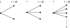
Discrete lattice is a stochastic process, where the stochastic variable can change only after passing certain time-step (stepping time) and can take on given number of new values. A given time period (T  − t ), during which the stochastic process is simulated, is divided into finite number of time steps where dt is the length of one discrete time step (time interval). For any discrete moment at time t has the stochastic process at t  + dt (i.e. after passing stepping time) finite possible number of values which can take on. According to the number of values at the end of stepping time we work with the following processes: binomial (at t  + dt takes on two values), trinomial (at t  + dt takes on three values) or multinomial (at t  + dt takes on n values), see Fig. 1 .

Figure 1. Discrete stochastic lattices (left-binomial, middle-trinomial, right-multinomial).

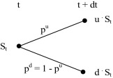
Simulation via binomial lattice is the simplest discrete process. Here, the value of underlying (random) asset takes on at time t the value S_t ; at the end of discrete interval (i.e. after passing stepping time) it can either jump up to ${\textstyle S_{t+dt}^{u}}$ or down to ${\textstyle S_{t+dt}^{d}}$ with some transition (risk-neutral) probability. If the process can take on only positive values (typical for most financial variables), we work with geometric version, where it holds for upward jump,

$S_{t+dt}^{u}=u\cdot S_{t}$

( 3.1)

and downward jump,

$S_{t+dt}^{d}=d\cdot S_{t}$

( 3.2)

and where u (d ) are up and down factors. For these two factors it holds following: u  ≥ 1; 0 < d  ≤ 1 and d  < e^r_fdt  < u . The upward and downward factors u and d and transition (risk-neutral) probabilities are set uniquely in order to determine the evolution of underlying asset. Due to the fact that expected return of any asset is assumed to be risk-free, the expected value at the end of discrete step equals S_t  · e^{r_f ·dt} . It follows that the expected value of the underlying asset can be written as,

$E(S_{t+dt})=S_{t}\cdot e^{r_{f}\cdot dt}=p^{u}\cdot u\cdot S_{t}+(1-p^{u})\cdot d\cdot S_{t}$

( 3.3)

and after some rearrangements,

$e^{r_{f}\cdot dt}=p^{u}\cdot u+(1-p^{u})\cdot d$

( 3.4)

From (3.4) the risk-neutral probability of upward jump p^u is given as,

$p^{u}={\frac {e^{r_{f}\cdot dt}-d}{u-d}}$

( 3.5)

and for downward jump must follows,

$p^{d}=(1-p^{u}){\mbox{.}}$

( 3.6)

The variance of the underlying asset between two subsequent discrete nodes at time t and t  + dt is σ²dt . And because the variance of random variable is generally given as σ² (S ) = E (S² ) − [E (S )]² , it is possible to write

$\sigma ^{2}dt=p^{u}\cdot u^{2}+(1-p^{u})\cdot d^{2}-[p^{u}\cdot u+(1-p^{u})\cdot d]^{2}{\mbox{.}}$

( 3.7)

Substituting for p^u from (3.5) , (3.6)  and (3.7) and after some rearrangements we get,

$\sigma ^{2}dt=e^{rf\cdot dt}\cdot (u+d)-u\cdot d-2\cdot e^{rf\cdot dt}{\mbox{.}}$

( 3.8)

Solving (3.4)  and (3.8) and under the condition,

$u={\frac {1}{d}}{\mbox{,}}$

( 3.9)

we get for upward and downward factors u and d following formulas,

$u=e^{\sigma \cdot {\sqrt {dt}}}{\mbox{,}}$

( 3.10)

$d=e^{-\sigma \cdot {\sqrt {dt}}}{\mbox{.}}$

( 3.11)

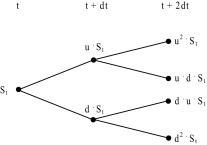
Fig. 2 shows one period binomial lattice with geometric process.

Figure 2. One period binomial lattice (geometric process).

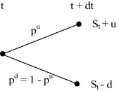
In situation, that the simulated process can take on both positive and negative values, we work with arithmetic version, where ${\textstyle S_{t+dt}^{u}=S_{t}+u}$ and ${\textstyle S_{t+dt}^{d}=S_{t}-d}$ , see Fig. 3 .²

Figure 3. One period binomial lattice (arithmetic process).

Simulation via binomial lattice with volatility change

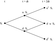
If we assume the constant volatility σ over the period (T  − t ), the up and downward factors given according to (3.10)  and (3.11) are constant throughout the whole lattice model and due to (3.9) it holds u  · d  = d  · u  = 1, which follows in the result the lattice recombines. This means that the nodes reconnect, i.e. S_{t +2dt}  = u  · d  · S_t or S_{t +2dt}  = d  · u  · S_t . Furthermore, the value of the underlying asset in any node of the binomial lattice can be expressed as,

$S_{t+i\cdot dt}=u^{j}\cdot d^{i-j}\cdot S_{t}$

( 3.12)

If (3.10)  and (3.11) are unchanged and under the assumption of constant risk-free rate, the transition probabilities between any two subsequent nodes according to (3.5)  and (3.6) are constant, as well. Fig. 4 illustrates two-period recombining binomial lattice can be depicted as it is shown in Fig. 4 .

Figure 4. Two-period recombining binomial lattice (geometric process).

When an up move followed by a down move does not reconnect in the same node as a down move followed by an up move, i.e. S_{t +2dt}  ≠ u  · d  · S_t or S_{t +2dt}  ≠ d  · u  · S_t , the lattice is called non-recombining. Non-recombining lattice is used for analysis when there are multiple sources of uncertainty or when volatility changes over time. The main difference between recombining and non-recombining lattice is, that the lattice with n periods the recombining have (n  + 1) final unique values, whereas non-recombining 2ⁿ values, which are not unique. Fig. 5 shows two-period non-recombining binomial lattice.

Figure 5. Two-period non-recombining binomial lattice (geometric process).

If the assumption of constant volatility is relaxed, it follows that upward and downward factors according to (3.10)  and (3.11) are not constant throughout the lattice any more. The same is true about the transition risk-neutral probabilities. In such situations, there are a few ways how to overcome this issue: (a) for each period and volatility calculate corresponding upward and downward factors; the same is true about the transition probabilities (b) set the transition probabilities p^u  = p^d  = 0.5 throughout the binomial lattice and calculate for each period upward and downward factors according to given volatility,

$u=e^{(r_{f}-\sigma ^{2}/2)\cdot dt+\sigma {\sqrt {dt}}}$

( 3.13)

$d=e^{(r_{f}-\sigma ^{2}/2)\cdot dt-\sigma {\sqrt {dt}}}$

( 3.14)

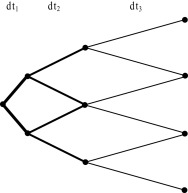
or (c) the size of up and down movements and their corresponding transition probabilities are constant throughout the lattice, but the time periods are of unequal length. When volatility is high, the time periods are short, so that the state variable changes frequently by the standardized amount. When volatility is lower, the periods are longer so that the changes in the state variable are less frequent.³ This binomial lattice is presented in Fig. 6 .

Figure 6. Three-period recombining binomial lattice with unequal length of time steps.

Application – valuation American real option valuation with changing volatility

This part of the paper is focused on the application of discrete binomial lattice on the real option valuation (option to expand a project). The option is an American-type option, i.e. the project can be expanded at any time during the expected life span. It is assumed that the underlying asset is the cash flow generated by the project; the initial value FCF₀  = 100 c.u., and evolves according to the GBM. Company has the option to expand the project at any time during the life span with the costs on expansion I_E  = 80 c.u. The risk-free rate is r_f  = 8% p.a. and the annual volatility σ  = 25%. The illustration example is structured as follows:

• first, it is assumed that the volatility is constant,
• next, volatility of cash flow increases as the project expected end-life is approaching,
• in the end, volatility of cash flow increases is assumed again, for problem solution, an approach suggested by Guthrie (2011) is employed.

Problem solution I

Problem solution is decomposed into the following steps:

• Calculation of upward and downward factor. Substituting into (3.10)  and (3.11) we get u  = 1.284 and d  = 0.7788.
• Calculation the risk-neutral probabilities. Applying (3.5)  and (3.6) we get following: p^u  = 60.27% and p^d  = 39.73%.
• Simulation of the underlying asset via the recombining and non-recombining lattice.
• The intrinsic value calculation. For option to expand it is defined as IV_t  = max(V_t  − I_E  ; 0).⁴
• Option value calculation according to (3.7) by applying backward-induction approach with risk-neutral probabilities.

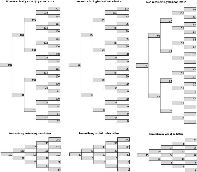
Following Fig. 7 shows numerical results; Fig. 8 shows the histogram of end node values for recombining and non-recombining lattice. The results obtained are identical no matter which approach is used (option value equals 45 c.u.).

Figure 7. Real option valuation lattice (recombining and non-recombining lattice, constant volatility).

Figure 8. End node values of underlying asset value for non-recombining lattice (left) and recombining lattice (right).

Problem solution II

Real option valuation with changing volatility includes following steps:

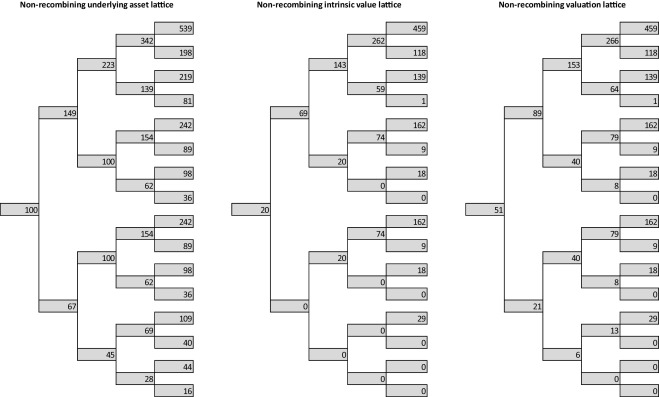
• Calculation of upward and downward factors for each period and volatility according to (3.10)  and (3.11) . Recall, that the volatility σ₁ applies for the first two periods, σ₂ for period three and σ₃ for period four. Results are summarized in the following Table 1 .

Table 1. Up (down) ward factors and transition probabilities for given volatility level.

	Volatility (%)	Period	Upward factor (u )	Downward factor (d )	pu (%)
σ1	40	0–1 and 1–2	1.4918	0.6703	50.3
σ2	45	3	1.5683	0.6376	47.9
σ2	50	4	1.6487	0.6065	45.7

• Simulation of the underlying asset via the recombining and non-recombining lattice.
• The intrinsic values calculation.
• Option value calculation according to (3.7) by applying backward-induction approach with risk-neutral probabilities.

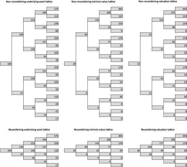
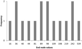
Fig. 9 shows resulting lattices; Fig. 10 shows the histogram of end node values for recombining and non-recombining lattice. The results obtained are no more identical; the difference is caused primarily by the larger differences in the end nodes values (and their frequencies) of the recombining and non-recombining underlying asset lattice.

Figure 9. Real option valuation lattice (recombining and non-recombining lattice, increasing volatility).

Figure 10. End node values for non-recombining lattice (left) and recombining lattice (right).

Problem solution III

Real option valuation with changing volatility includes following steps:

• Calculation of the upward and downward factors for each period and volatility according to (3.13)  and (3.14) ; the transition probability is set to equals 50% for all periods, see Table 2 .

Table 2. Up (down) ward factors and transition probabilities for given volatility level.

	Volatility (%)	Period	Upward factor (u )	Downward factor (d )	pu (%)
σ1	40	0–2	1.4918	0.6703	50
σ2	45	3	1.5353	0.6242	50
σ2	50	4	1.5762	0.5798	50

• Simulation of the underlying asset via the non-recombining lattice. Due to the fact that the u  · d  ≠ 1, it is not possible to construct the recombining lattice.
• The intrinsic value calculation.
• Option valuation according to (3.7) by backward-induction approach and applying risk-neutral probabilities.

Results are again depicted in the following Fig. 11 ; Fig. 12 shows frequency of underlying asset end node values. It is apparent that this approach provides the same results as the one applied in Problem solution II.⁵

Figure 11. Real option valuation lattice (non-recombining lattice, increasing volatility).

Figure 12. End node values of underlying asset for non-recombining lattice.

Conclusion

This paper focuses at the real option valuation under changing volatility. Change in the volatility structure (i.e. change in project cash flows riskiness) is a typical feature for most of the long-term project, where the prediction of the cash flows in the far future is difficult and associated with the higher risk.

Due to the fact that most real options are American-style options, there are discrete binomial models applied. Moreover, other option valuation models (like B–S model) rely on some assumptions (valuation European-style options, constant volatility, risk free rate) and their application may be limited for real options issues solutions.

It has been shown that, under changing volatility application of non-recombining lattice with risk-neutral probabilities is a useful tool helping the analysts to overcome the option-valuation problems associated with the variable parameters.

There were two approaches employed to evaluate real option with the volatility change. The former one is based on the assumption that the entire lattice is divided into stages with constant volatility; at the end of the constant volatility period, each resulting point becomes starting point of a new lattice. For each period, corresponding up and down factors and transition probabilities must be calculated. The latter approach sets the transition probabilities to 50% throughout the entire lattice and adjusts the up and downward factors with respect to the volatility during given period. Due to the fact that the centrality is broken, only non-recombining lattice can be used. Anyway, for sufficient number of steps both approaches provide the same results.

Conflict of interest

The author declares that there is no conflict of interest.

Acknowledgements

This paper was supported within Operational Programme Education for Competitiveness – Project No. CZ.1.07/2.3.00/20.0296 and the Project No. GP14-15175P.

References

1. Black and Scholes, 1973 F. Black, M. Scholes; The pricing of options and corporate liabilities; J. Polit. Econ., 81 (3) (1973), pp. 637–654
2. Brach, 2002 M.A. Brach; Real Options in Practice; Wiley, New Jersey (2002)
3. Brennan and Schwartz, 1985 M.J. Brennan, E.S. Schwartz; Evaluating natural resource investments; J. Bus., 58 (2) (1985), pp. 135–157
4. Brennan and Trigeorgis, 2000 M.J. Brennan, L. Trigeorgis; Project Flexibility Agency and Competition: New Developments in the Theory and Application of Real Options; (first ed.)Oxford University Press, London (2000)
5. Copeland and Antikarov, 2003 T.E. Copeland, V. Antikarov; Real Options Revised Edition: A Practitioners Guide; (second ed.)Texere, New York (2003)
6. Cox et al., 1979 J.C. Cox, S.A. Ross, M. Rubinstein; Option pricing: a simplified approach; J. Financ. Econ., 7 (3) (1979), pp. 229–263
7. Damodaran, 2006 A. Damodaran; Damodaran on Valuation: Security Analysis for Investment and Corporate Finance; (second ed.)Wiley, New Jersey (2006)
8. Dixit and Pindyck, 1994 A.K. Dixit, R.S. Pindyck; Investment under Uncertainty; (first ed.)Princeton University Press, New York (1994)
9. Grenadier, 2000 S. Grenadier; Game Choices: The Intersection of Real Options and Game Theory; Riskbooks, London (2000)
10. Guthrie, 2011 G. Guthrie; Learning options and binomial trees; Wilmott J., 3 (1) (2011), pp. 1–23
11. Haahtela, 2010 T. Haahtela; Recombining trinomial tree for real option valuation with changing volatility; Annual Real Option Conference (2010)
12. Hoek and Elliot, 2006 J. Hoek, R.J. Elliot; Binomial Models in Finance; Springer, New York (2006)
13. Hull, 2014 J.C. Hull; Options, Futures, and Other Derivatives; (ninth ed.)Prentice Hall (2014)
14. Merton, 1973 R. Merton; The theory of rational option pricing; Bell J. Econ. Manag. Sci., 4 (1) (1973), pp. 141–183
15. Mun, 2005 J. Mun; Real Option Analysis. Tool and Techniques for Valuing Strategic Investments and Decisions; (second ed.)Wiley, New Jersey (2005)
16. Mun, 2003 J. Mun; Real Options Analysis Course: Business Cases and Software Applications; Wiley, New Jersey (2003)
17. Smith and Nau, 1995 J.E. Smith, R.F. Nau; Valuing risky projects: option pricing theory and decision analysis; Manag. Sci., 14 (1995), pp. 795–816
18. Tichý, 2008 T. Tichý; Lattice Models. Pricing and Hedging at (In)omplete Markets; VŠB-TU Ostrava (2008)
19. Trigeorgis, 1999 L. Trigeorgis; Real Options and Business Strategy: Applications to Decision Making; Riskbooks, London (1999)
20. Trigeorgis and Schwartz, 2001 L. Trigeorgis, E.S. Schwartz; Real Options and Investments under Uncertainty; MIT Press, Cambridge (2001)
21. Trigeorgis and Smith, 2004 L. Trigeorgis, H.T.J. Smith; Strategic Investment: Real Options and Games; Princeton University Press, New York (2004)

Notes

1. More details are available in Hoek and Elliot (2006) .

2. More details on derivation can be found in Tichý (2008) , Hull (2014) , etc.

3. For more details and mathematical background see Guthrie (2011) or Haahtela (2010) .

4. For more details see for example Trigeorgis (1999) , Trigeorgis (2000) Mun (2003) or Mun (2005) .

5. Small difference in the results is caused by the number of the steps in valuation lattice. For five and more steps the results world be identical.