Finite volume for stress analysis upon polygonal, unstructured and non conforming meshes

Abstract

Within this paper we discuss a numerical strategy to solve the elasticity problem upon unstructured and non conforming meshes, allowing all kinds of flat-faced elements (polygons in 2D and polyhedra in 3D). The core of the formulation relies on two numerical procedures 1) the Control Volume Function Approximation (CVFA), and 2) the polynomial interpolation in the neighborhood of the control volumes, which is used to solve the surface integrals resulting from applying the divergence theorem. By comparing the estimated stress against the analytical stress field of the well known test of an infinite plate with a hole, we show that this conservative approach is robust and accurate.

Keywords: Stress analysis, elasticity, solid mechanics, CVFA, Finite Volume, unstructured mesh, non conforming mesh

1. Introduction

One of the main aims in engineering is creating tools, structures and systems to enhance the quality of life in our society. In the course of the creation process, the design stage is critical for the final outcome. During this stage the engineer have to predict the prototype response when interacting with the physical world. Many of the observed phenomena in the physical world, such as solid mechanics, fluid dynamics, heat diffusion, and others, can be described with Partial Differential Equations (PDEs) by assuming time and space as a continuum.

Computational Continuum Mechanics (CCM) is the area dedicated to develop numerical methods and heuristics to solve these PDEs. Most of the methods can be classified into these two families: 1) weighted residual and 2) conservative methods. The Galerkin formulations are popular and widely used weighted residual methods, such as the Finite Element Method (FEM), which is a well established technique in Computational Solid Mechanics (CSM). Alternatively, the Finite Volume Method (FV) and the Control Volume Function Approximation (CVFA) are common approaches of conservative methods. The main difference between both families is that weighted residuals methods do not conserve quantities locally, but globally instead, resulting in linear systems with commendable numerical properties (symmetrical and well-conditioned matrices, for example). Nevertheless, due to its conservative nature, the second group is more attractive for fluid structure interaction [1,2] and multiphysics simulations [3,4], where several PDE-solvers must be coupled. For that reason, in recent years FV has been subject of interest for solving CSM problems.

Most of the CSM non-linear strategies depend on the accuracy of the estimated stress field for the elasticity problem, such as those for plasticity and damage [5,6]. Hereafter we refer as elasticity-solver to the numerical computation that calculates the displacement and stress fields for a given domain and boundary conditions.

In his influential papers, Oñate et al. propose a FV format for structural mechanics based on triangular meshes [7,8], discussing the cell vertex scheme, the cell centred finite volume scheme and its corresponding mixed formulations, showing that the cell centred strategy produces the same symmetrical global stiffness matrix that FEM using linear triangular elements. Analogously, Bailey et al. develop a similar approach, but using quadrilateral elements to produce cell-centred volumes [9,10]. Even though, the shapes of the volumes in both formulations are completely defined by the FEM-like mesh (triangular or quadrilateral) and it is not possible to handle arbitrary polygonal shapes, as we might expect when receiving the mesh as a read-only input.

Slone et al. [11] extends the investigation of [7] by developing a dynamic solver based on an implicit Newmark scheme for the temporal discretization, with the motivation of coupling an elasticity-solver with his multi-physics modelling software framework, for later application to fluid structure interaction.

Another remarkable algorithm is the proposed by Demirdzic et al. [12,13,14,15,16]. The numerical procedure consists in decoupling the strain term into the displacement Jacobian and its transpose in a cell-centred scheme. The Jacobian is implicitly estimated by approximating the normal component of each face as the finite difference with respect to the adjacent nodes, while the Jacobian transpose is an explicit average of Taylor approximations around the same adjacent nodes. This decoupling produces a smaller memory footprint than FEM because the stiffness matrix is the same for all the components. The solution is found by solving one component each iteration in a coordinate descent minimization. This line of work has shaped most of the state of the art techniques in FV for coupling elasticity-solvers to Computational Fluid Dynamics (CFD) via finite volume practices (usually associated to CFD), such as the schemes proposed by [17,18,19]. However, this segregated algorithm may lead to slow convergence rates when processing non-linear formulations, for example, when it is required to remove the positive principal components of the stress tensor in phase-field damage formulations [20]. In addition, if some non-linear strategy requires multiple iterations of the linear elasticity-solver, such as finite increments in damage models, the nested iterations will increase the processing requirements for simple problems. To circumvent this drawback Cardiff et al. presents a fully block coupled direct solution procedure [21], which does not require multiple iterations, at expense of decomposing the displacement Jacobian of any arbitrary face into a) the Jacobian of the displacement normal component, b) the Jacobian of the displacement tangential component, c) the tangential derivative of the displacement normal component and d) the tangential derivative of the displacement tangential component. This decomposition complicates the treatment of the stress tensor in the iterative non-linear solvers mentioned before for plasticity and damage.

A generalized finite volume framework for elasticity problems on rectangular domains is proposed by Cavalcante et al. [22]. They use higher order displacement approximations at the expense of fixed axis-aligned grids for discretization.

Nordbotten proposes a generalization of the multi-point flux approximation (MPFA), which he names multi-point stress approximation (MPSA) [23]. The MPSA assembles unique linear expressions for the face average stress with more than two points in order to capture the tangential derivatives. The stress field calculated with this procedure is piece-wise constant.

In this work, we propose an elasticity-solver based on CVFA techniques [24,25], using piece-wise polynomial interpolators for solving the surface integrals on the volumes boundaries. The polynomials degree can be increased without incrementing the system degrees of freedom, which make this method more suitable for non-linear models and dynamic computations. Furthermore, this algorithm can handle polygonal/polyhedral, unstructured and non conforming meshes, and does not require the decomposition of the stress tensor.

2. Mathematical model

We consider an arbitrary body, ${\textstyle \Omega \in \mathbb {R} ^{\hbox{dim}}}$, with boundary ${\textstyle \partial \Omega }$. The displacement of a point ${\textstyle \mathbf {x} \in \Omega }$ is denoted by ${\textstyle {\boldsymbol {u}}(\mathbf {x} )\in \mathbb {R} ^{\hbox{dim}}}$. The subscript brackets ${\textstyle (\cdot )_{[]}}$ indicates the component of the vector or matrix. By assuming small deformations and deformation gradients, the infinitesimal strain tensor, denoted ${\textstyle {\boldsymbol {\varepsilon }}(\mathbf {x} )\in \mathbb {R} ^{{\hbox{dim}}\times {\hbox{dim}}}}$, is given by

${\boldsymbol {\varepsilon }}={\frac {1}{2}}\left(\nabla {\boldsymbol {u}}+\left[\nabla {\boldsymbol {u}}\right]^{T}\right).$

(1)

Moreover, by considering isotropic elastic materials, the stress tensor, ${\textstyle {\boldsymbol {\sigma }}(\mathbf {x} )\in \mathbb {R} ^{{\hbox{dim}}\times {\hbox{dim}}}}$, is defined as

${\boldsymbol {\sigma }}=2\mu {\boldsymbol {\varepsilon }}+\lambda tr({\boldsymbol {\varepsilon }})\mathbf {I} ,$

(2)

where ${\textstyle \mathbf {I} }$ is the identity matrix, ${\textstyle tr(\cdot )}$ is the trace, and ${\textstyle \lambda }$ and ${\textstyle \mu }$ are the Lamé parameters characterizing the material. These parameters are related with the Young's modulus, ${\textstyle E}$, and the Poisson's ratio, ${\textstyle \nu }$, by the following equivalences

$\mu ={\frac {E}{2(1+\mu )}},$

(3)

and

$\lambda ={\frac {\nu E}{(1+\nu )(1-\lambda _{\nu })}},$

(4)

where ${\textstyle \lambda _{\nu }=\nu }$ for plane stress analysis, and ${\textstyle \lambda _{\nu }=2\nu }$ for plane strain and the 3D cases.

The strong form of the static linear elasticity equation is

$\nabla \cdot {\boldsymbol {\sigma }}=0,$

(5)

The domain boundary ${\textstyle \partial \Omega =\Gamma _{N}\cup \Gamma _{D}}$ is the union of the boundary with Neumann conditions, denoted ${\textstyle \Gamma _{N}}$, and the boundary with Dirichlet conditions, denoted ${\textstyle \Gamma _{D}}$. Equation (5) must be satisfied for the given forces ${\textstyle {\boldsymbol {b}}_{N}}$ and displacements ${\textstyle {\boldsymbol {u}}_{D}}$ along the boundary. The following equations remark these user defined boundary conditions,

${\boldsymbol {\sigma }}\mathbf {n} ={\boldsymbol {b}}_{N}(\mathbf {x} ),\mathbf {x} \in \Gamma _{N},$ (6.a) ${\boldsymbol {u}}={\boldsymbol {u}}_{D}(\mathbf {x} ),\mathbf {x} \in \Gamma _{D},$ (6.b)

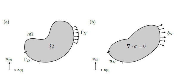
Figure 1 illustrates the initial body with the boundary conditions, and the distorted body after equilibrium is solved in the elasticity equation.

Figure 1. (a) The initial body, $\Omega$, with its boundary conditions $\partial \Omega =\Gamma _{N}\cup \Gamma _{D}$. (b) The distorted body resulting from solving equilibrium in the elasticity equation, with the boundary conditions given by ${\boldsymbol {b}}_{N}$ and ${\boldsymbol {u}}_{D}$. The boundaries where there are not conditions indicated explicitly, correspond to Neumann conditions ${\boldsymbol {b}}_{N}=0$

3. Numerical method

On this section we go into the details of the numerical procedure by discussing: 1) the discretization with CVFA, 2) the control volumes integration, 3) the subfaces integrals, 4) the simplex-wise polynomial approximation, 5) the pair-wise polynomial approximation, 6) the homeostatic splines used within the shape functions, 7) the linear system assembling, 8) how to impose boundary conditions and 9) two special cases of the formulation.

For the sake of legibility, in some parts of the text we unfold the matrices only for the bidimensional case, but the very same procedures must be followed for the 3D case.

3.1 Discretization of domain into control volumes

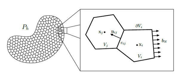
The domain ${\textstyle \Omega }$ is discretized into ${\textstyle N}$ control volumes, denoted ${\textstyle V_{i}}$, using the Control Volume Function Approximation (CVFA) proposed by Li et al. [24,25]. The partition ${\textstyle P_{h}}$ of ${\textstyle \Omega }$ is defined by

$P_{h}=\bigcup _{i=1}^{N}V_{i},~~~{\hbox{with}}~~~V_{i}\cap V_{j}=\emptyset ,~~~i\neq j,$

(7)

where the boundary of each control volume, ${\textstyle \partial V_{i}}$, is composed by ${\textstyle N_{i}}$ flat faces, denoted ${\textstyle e_{ij}}$,

$\partial V_{i}=\bigcup _{j=1}^{N_{i}}e_{ij},~~~{\hbox{with}}~~~e_{ij}\cap e_{ik}=\emptyset ,~~~j\neq k.$

(8)

Figure 2 illustrates the partition ${\textstyle P_{h}}$ of ${\textstyle \Omega }$ into ${\textstyle N}$ control volumes defined in the equations (7) and (8).

Figure 2. The partition $P_{h}$ is the discretization of the domain $\Omega$ into $N$ control volumes. The boundary of the control volumes, $\partial V_{i}$, is conformed by $N_{i}$ flat faces, denoted $e_{ij}$. The unit vector $\mathbf {n} _{ij}$ is normal to the face $e_{ij}$. The faces of the volumes adjacent to the boundary $\Gamma _{N}$ are integrated using the condition ${\boldsymbol {b}}_{N}$

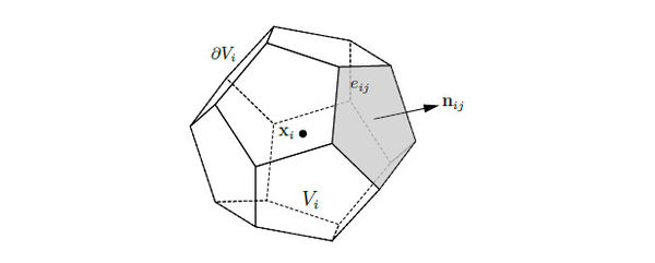
Figure 3 shows a three dimensional control volume.

Figure 3. The boundary $\partial V_{i}$ of the three dimensional control volume $V_{i}$ is subdivided into $N_{i}$ flat faces, denoted $e_{ij}$. The unit vector $\mathbf {n} _{ij}$ is normal to the face $e_{ij}$

Every control volume ${\textstyle V_{i}}$ must have a calculation point

$\mathbf {x} _{i}\in V_{i}\cup \partial V_{i},$

(9)

which is used to estimate the displacement field. Such a point is the base location to calculate the stiffness of the volume. In the volumes adjacent to the boundary ${\textstyle \Gamma _{D}}$, it is convenient to establish the calculation point over the corresponding boundary face,

$\mathbf {x} _{i}\in \partial V_{i}\cap \Gamma _{D},$

(10)

in order to set the Dirichlet condition directly on the point.

3.2 Control volumes integration

The elasticity equation (5) is now integrated over the control volume

$\int _{V_{i}}\nabla \cdot {\boldsymbol {\sigma }}~dV=0,$

(11)

using the divergence theorem we transform the volume integral into a surface integral over the volume boundary

$\int _{\partial V_{i}}{\boldsymbol {\sigma }}\mathbf {n} ~dS=0.$

(12)

The evaluation of the surface integrals is based on the approximation of the displacement field inside the neighborhood of the volume, denoted ${\textstyle {B}_{i}}$,

${\boldsymbol {u}}_{i}(\mathbf {x} )=\sum \limits _{q\in {B}_{i}}\varphi _{q}\mathbf {x} _{q},$

(13)

making use of a group of piece-wise polynomial interpolators, denoted ${\textstyle \varphi _{q}}$. We are going to discuss these interpolators later in this section.

For that reason, the displacement field is decoupled from the stress tensor by using the strain (1) and stress (2) definitions. Taking advantage of the stress tensor symmetry ${\textstyle ~{\boldsymbol {\sigma }}}$, we rewrite the stress normal to the boundary as

${\boldsymbol {\sigma }}\mathbf {n} ={\begin{bmatrix}{\boldsymbol {\sigma }}_{[11]}&{\boldsymbol {\sigma }}_{[12]}\\{\boldsymbol {\sigma }}_{[12]}&{\boldsymbol {\sigma }}_{[22]}\end{bmatrix}}{\begin{bmatrix}\mathbf {n} _{[1]}\\\mathbf {n} _{[2]}\end{bmatrix}}={\begin{bmatrix}\mathbf {n} _{[1]}&&\mathbf {n} _{[2]}\\&\mathbf {n} _{[2]}&\mathbf {n} _{[1]}\end{bmatrix}}{\begin{bmatrix}{\boldsymbol {\sigma }}_{[11]}\\{\boldsymbol {\sigma }}_{[22]}\\{\boldsymbol {\sigma }}_{[12]}\end{bmatrix}}=\mathbf {T} {\vec {\boldsymbol {\sigma }}},$

(14)

where ${\textstyle \mathbf {T} }$ is the face orientation matrix and ${\textstyle ~{\vec {\boldsymbol {\sigma }}}}$ is the engineering stress vector. Developing the stress definition (2) component-wise we can decompose it into the constitutive matrix, denoted ${\textstyle \mathbf {D} }$, and the engineering strain vector, denoted ${\textstyle {\vec {\boldsymbol {\varepsilon }}}}$, as follows

${\vec {\boldsymbol {\sigma }}}={\begin{bmatrix}{\boldsymbol {\sigma }}_{[11]}\\{\boldsymbol {\sigma }}_{[22]}\\{\boldsymbol {\sigma }}_{[12]}\end{bmatrix}}={\begin{bmatrix}2\mu ~{\boldsymbol {\varepsilon }}_{[11]}+\lambda \left({\boldsymbol {\varepsilon }}_{[11]}+{\boldsymbol {\varepsilon }}_{[22]}\right)\\2\mu ~{\boldsymbol {\varepsilon }}_{[22]}+\lambda \left({\boldsymbol {\varepsilon }}_{[11]}+{\boldsymbol {\varepsilon }}_{[22]}\right)\\2\mu ~{\boldsymbol {\varepsilon }}_{[12]}\end{bmatrix}}$ (15) $={\begin{bmatrix}\left(2\mu +\lambda \right)&\lambda &\\\lambda &\left(2\mu +\lambda \right)&\\&&\mu \end{bmatrix}}{\begin{bmatrix}{\boldsymbol {\varepsilon }}_{[11]}\\{\boldsymbol {\varepsilon }}_{[22]}\\2{\boldsymbol {\varepsilon }}_{[12]}\end{bmatrix}}=\mathbf {D} {\vec {\boldsymbol {\varepsilon }}},$ (16)

then the components of the strain vector are retrieved from the equation (1), and it is decomposed into the matrix differential operator ${\textstyle \mathbf {S} }$ and the displacement function ${\textstyle {\boldsymbol {u}}}$.

${\vec {\boldsymbol {\varepsilon }}}={\begin{bmatrix}{\boldsymbol {\varepsilon }}_{[11]}\\{\boldsymbol {\varepsilon }}_{[22]}\\2{\boldsymbol {\varepsilon }}_{[12]}\end{bmatrix}}={\begin{bmatrix}\displaystyle {\frac {\partial {\boldsymbol {u}}_{[1]}}{\partial \mathbf {x} _{[1]}}}\\\displaystyle {\frac {\partial {\boldsymbol {u}}_{[2]}}{\partial \mathbf {x} _{[2]}}}\\\displaystyle {\frac {\partial {\boldsymbol {u}}_{[1]}}{\partial \mathbf {x} _{[2]}}}+\displaystyle {\frac {\partial {\boldsymbol {u}}_{[2]}}{\partial \mathbf {x} _{[1]}}}\end{bmatrix}}={\begin{bmatrix}\displaystyle {\frac {\partial }{\partial \mathbf {x} _{[1]}}}&\\&\displaystyle {\frac {\partial }{\partial \mathbf {x} _{[2]}}}\\\displaystyle {\frac {\partial }{\partial \mathbf {x} _{[2]}}}&\displaystyle {\frac {\partial }{\partial \mathbf {x} _{[1]}}}\end{bmatrix}}{\begin{bmatrix}{\boldsymbol {u}}_{[1]}\\{\boldsymbol {u}}_{[2]}\end{bmatrix}}=\mathbf {S} {\boldsymbol {u}},$

(17)

Summarizing the equations (14), (16) and (17) we have

${\boldsymbol {\sigma }}\mathbf {n} =\mathbf {T} {\vec {\boldsymbol {\sigma }}}=\mathbf {T} \mathbf {D} {\vec {\boldsymbol {\varepsilon }}}=\mathbf {T} \mathbf {D} \mathbf {S} {\boldsymbol {u}},$

(18)

where ${\textstyle \mathbf {T} \mathbf {D} \mathbf {S} }$ is the stiffness of the volume boundary.

Once the displacement field is decoupled, we rewrite the equation (12) as

$\int _{\partial V_{i}}\mathbf {T} \mathbf {D} \mathbf {S} {\boldsymbol {u}}~dS=0.$

(19)

Using the fact that the control volume boundary is divided into flat faces, as in equation (8), we split the integral (19) into the sum of the flat faces integrals

$\sum \limits _{j=1}^{N_{i}}\int _{e_{ij}}\mathbf {T} \mathbf {D} \mathbf {S} {\boldsymbol {u}}~dS=0.$

(20)

Notice that the face orientation ${\textstyle \mathbf {T} }$ along the flat face, denoted ${\textstyle \mathbf {T} _{ij}}$, is constant. Furthermore, if the control volumes are considered to be made of a unique material and the flat faces to be formed by pairs of adjacent volumes, then the constitutive matrix ${\textstyle \mathbf {D} }$ along the flat face, denoted ${\textstyle \mathbf {D} _{ij}}$, is also considered constant. The matrix ${\textstyle \mathbf {D} _{ij}}$ is estimated from the harmonic average of the Lamé parameters assigned to the adjacent volumes, where ${\textstyle \lambda _{i}}$ and ${\textstyle \mu _{i}}$ are the properties of the volume ${\textstyle V_{i}}$,

$\mu _{ij}={\frac {2\mu _{i}\mu _{j}}{\mu _{i}+\mu _{j}}}~~~~{\hbox{and}}~~~~\lambda _{ij}={\frac {2\lambda _{i}\lambda _{j}}{\lambda _{i}+\lambda _{j}}},$

(21)

with ${\textstyle \mathbf {T} _{ij}}$ and ${\textstyle \mathbf {D} _{ij}}$ we simplify the equation (20) as

$\sum \limits _{j=1}^{N_{i}}\mathbf {T} _{ij}\mathbf {D} _{ij}\mathbf {H} _{ij}=0,$

(22)

where ${\textstyle \mathbf {H} _{ij}}$ is the strain integral along the flat face ${\textstyle e_{ij}}$,

$\mathbf {H} _{ij}=\int _{e_{ij}}\mathbf {S} {\boldsymbol {u}}~dS.$

(23)

The accuracy of the method depends on the correct evaluation of this integral.

3.3 Calculating face integrals

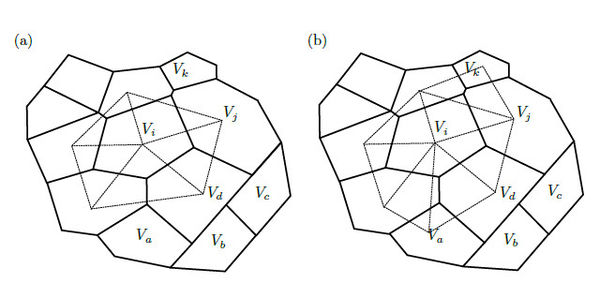
The surface integrals ${\textstyle \mathbf {H} _{ij}}$ along the flat faces ${\textstyle e_{ij}}$ are calculated using an auxiliary piece-wise polynomial approximation of the displacement field. This approximation is based on the simplices (triangles in 2D or tetrahedra in 3D) resulting from the Delaunay triangulation of the calculation points ${\textstyle \mathbf {x} _{i}}$ from the neighborhood of ${\textstyle V_{i}}$. The Delaunay triangulation is the best triangulation for numerical interpolation, since it maximizes the minimum angle of the simplices, which means that its quality is maximized as well. We define the neighborhood ${\textstyle {B}_{i}}$ of volume ${\textstyle V_{i}}$ as the minimum set of calculation points ${\textstyle \mathbf {x} _{j}}$ such that the simplices intersecting ${\textstyle V_{i}}$ does not change if we add another calculation point to the set. Observe that the neighborhood ${\textstyle {B}_{i}}$ does not always coincide with the set of calculation points in volumes adjacent to ${\textstyle V_{i}}$, as in most of the FV formulations. Once the neighborhood ${\textstyle {B}_{i}}$ is triangulated, we ignore the simplices with angles smaller than ${\textstyle 10}$ degrees, and the simplices formed outside the domain, which commonly appear in concavities of the boundary ${\textstyle \partial \Omega }$. The local set of simplices resulting from the neighborhood of ${\textstyle V_{i}}$ is denoted ${\textstyle P_{\alpha }}$. Figure 4 illustrates the difference between (a) the simplices resulting from the triangulation of the calculation points in adjacent volumes and (b) those resulting from the triangulation of the proposed neighborhood ${\textstyle {B}_{i}}$.

Figure 4. (a) The dotted line illustrates the triangulation of the calculation points of adjacent volumes to $V_{i}$, used by most of the FV methods. (b) The dotted line shows the simplices forming the piece-wise approximation used to solve the integrals $\mathbf {H} _{ij}$ of the control volume $V_{i}$

The face ${\textstyle e_{ij}}$ is subdivided into ${\textstyle N_{ij}}$ subfaces, denoted ${\textstyle e_{ijk}}$,

$e_{ij}=\bigcup \limits _{k=1}^{N_{ij}}e_{ijk},~~~{\hbox{with}}~~~e_{ijk}\cap e_{ijl}=\emptyset ,~~~l\neq k,$

(24)

these subfaces result from the intersection between ${\textstyle P_{\alpha }}$ and the control volume ${\textstyle V_{i}}$. Figure 4(b) illustrates six key points of this approach: 1) the simplices are used to create a polynomial interpolation of ${\textstyle {\boldsymbol {u}}(\mathbf {x} )}$ over the boundary of the control volume, 2) most of the faces are intersected by several simplices, such faces must be divided into subfaces to be integrated, 3) some few faces are inside a single simplex, as illustrated in the face formed by ${\textstyle V_{i}}$ and ${\textstyle V_{k}}$, 4) there are volumes that require information of non-adjacent volumes to calculate its face integrals, such as ${\textstyle V_{i}}$ requires ${\textstyle V_{k}}$, 5) the dependency between volumes is not always symmetric, which means that if ${\textstyle V_{i}}$ requires ${\textstyle V_{k}}$ does not implies that ${\textstyle V_{k}}$ requires ${\textstyle V_{i}}$, and 6) non conforming meshes are supported, as shown in the faces formed by ${\textstyle V_{a}}$, ${\textstyle V_{b}}$, ${\textstyle V_{c}}$, ${\textstyle V_{d}}$ and ${\textstyle V_{j}}$.

The integral (23) is now rewritten in terms of the subfaces

$\mathbf {H} _{ij}=\sum \limits _{k=1}^{N_{ij}}~\int _{e_{ijk}}\mathbf {S} {\boldsymbol {u}}~dS,$

(25)

Each subface ${\textstyle e_{ijk}}$ is bounded by a simplex, where the displacement ${\textstyle {\boldsymbol {u}}_{ijk}}$, and it derivatives, ${\textstyle ~(\mathbf {S} {\boldsymbol {u}})_{ijk}}$, are a polynomial interpolation. Hence the integrals in equation (25) are solved exactly by using the Gauss-Legendre quadrature with the required number of integration points, denoted ${\textstyle N_{g}}$, depending on the polynomial degree,

$\int _{e_{ijk}}\mathbf {S} {\boldsymbol {u}}~dS=\sum \limits _{g=1}^{N_{g}}~~w_{g}(\mathbf {S} {\boldsymbol {u}})_{ijk}|_{\mathbf {x} _{g}}.$

(26)

where ${\textstyle w_{g}}$ is the corresponding quadrature weight and ${\textstyle (\mathbf {S} {\boldsymbol {u}})_{ijk}|_{\mathbf {x} _{g}}}$ is the strain evaluation of the Gauss point with the proper change of interval, denoted ${\textstyle \mathbf {x} _{g}}$. Figure 5 shows the change of interval required for a 2D face. A 3D face (a polygon) must be subdivided to be integrated with a triangular quadrature.

Figure 5. (a) The shaded volume $V_{i}$ is being integrated. The integral over the subface $e_{ijk}$ is calculated using the polynomial approximation of the shaded simplex. The integration point must be mapped to (b) the normalized space $[-1,1]$ in order to use the Gauss- Legendre quadrature

Most of the cases, the displacement ${\textstyle ~{\boldsymbol {u}}_{ijk}}$ is interpolated inside the simplices, but in some geometrical locations these can not be created, in consequence, the displacement ${\textstyle ~{\boldsymbol {u}}_{ijk}}$ is interpolated pair-wise using the volumes adjacent to the subface ${\textstyle ~e_{ijk}}$. We discuss both strategies in the following subsections.

3.4 Simplex-wise polynomial approximation

In the general case, the simplices are formed by ${\textstyle ~({\hbox{dim}}+1)~}$ points. The points forming the simplex that is bounding the subface ${\textstyle e_{ijk}}$ are denoted ${\textstyle \mathbf {x} _{q}}$, and its displacements ${\textstyle {\boldsymbol {u}}_{q}}$.

The shape functions used for the polynomial interpolation are defined into the normalized space. A point in such space is denoted ${\textstyle {\boldsymbol {\xi }}}$, its ${\textstyle d^{th}}$ component is denoted ${\textstyle {\boldsymbol {\xi }}_{[d]}}$, and the ${\textstyle q^{th}}$ point forming the simplex is expressed ${\textstyle {\boldsymbol {\xi }}_{q}}$. The nodes of the normalized simplex are given by the origin, ${\textstyle {\boldsymbol {0}}}$, and the standard basis vectors,

${\boldsymbol {\xi }}_{q}=\left\{{\begin{array}{rl}\mathbf {e} _{q},&{\hbox{ for}}~~q\in [1,{\hbox{ dim}}],\\{\boldsymbol {0}},&{\hbox{ if}}~~q={\hbox{ dim}}+1\end{array}}\right.$

(27)

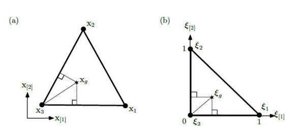
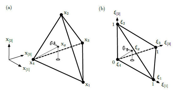
where ${\textstyle \mathbf {e} _{q}}$ is the ${\textstyle q^{th}}$ standard basis vector. Figures 6 and 7 illustrates the original and the normalized simplices with the corresponding node numeration for 2D and 3D respectively.

Figure 6. (a) The simplex formed by the points $\mathbf {x} _{1}$, $\mathbf {x} _{2}$ and $\mathbf {x} _{3}$ in the original space contains an interior point $\mathbf {x} _{g}$ that is mapped to (b) ${\boldsymbol {\xi }}_{g}$ into the normalized 2D-simplex formed by the points ${\boldsymbol {\xi }}_{1}$, ${\boldsymbol {\xi }}_{2}$ and ${\boldsymbol {\xi }}_{3}$

Figure 7. (a) The 3D-simplex formed by the points $\mathbf {x} _{1}$, $\mathbf {x} _{2}$, $\mathbf {x} _{3}$ and $\mathbf {x} _{4}$ in the original space contains an interior point $\mathbf {x} _{g}$ that is mapped to (b) ${\boldsymbol {\xi }}_{g}$ into the normalized 3D-simplex formed by the points ${\boldsymbol {\xi }}_{1}$, ${\boldsymbol {\xi }}_{2}$, ${\boldsymbol {\xi }}_{3}$ and ${\boldsymbol {\xi }}_{4}$

The shape functions, denoted ${\textstyle \varphi _{q}}$, are used to interpolate the displacement field inside the normalized simplex. Such functions are non-negative and are given by

${P}_{c}\left({\boldsymbol {\xi }}_{[q]}\right),~~~{\hbox{ if}}~~q\in [1,{\hbox{ dim}}],$ (28.a) $1-\sum \limits _{d=1}^{\hbox{dim}}{P}_{c}\left({\boldsymbol {\xi }}_{[d]}\right),~~~{\hbox{ for}}~~q={\hbox{ dim}}+1,$ (28.b)

where ${\textstyle {P}_{c}(\cdot )}$ is the homeostatic spline, which is the simplest polynomial defined in the interval ${\textstyle [0,1]}$ that have ${\textstyle ~c~}$ derivatives equal to zero in the endpoints of the interval. We will discuss this spline later.

The set of shape functions is a partition of unity, which means that the sum of the functions in the set is equal to one into the interpolated domain

$\sum \limits _{q=1}^{{\hbox{dim}}+1}\varphi _{q}({\boldsymbol {\xi }})=1~~~~{\hbox{for any }}{\boldsymbol {\xi }}{\hbox{ inside the simplex,}}$

(29)

furthermore, these functions are equal to one in its corresponding node, which implies that

$\varphi _{q}({\boldsymbol {\xi }}_{q})=1~~~~{\hbox{ for any }}{\boldsymbol {\xi }}_{q}{\hbox{ forming the simplex,}}$ (30) $\varphi _{q}({\boldsymbol {\xi }}_{p})=0~~~~{\hbox{ for any }}{\boldsymbol {\xi }}_{p}\neq {\boldsymbol {\xi }}_{q}{\hbox{ forming the simplex,}}$ (31)

The gradients of the shape functions with respect to the normalized space are denoted ${\textstyle \nabla _{\boldsymbol {\xi }}\varphi _{q}}$. The norm of the sum of such gradients is zero

$\left|\left|\sum \limits _{q=1}^{{\hbox{dim}}+1}\nabla _{\boldsymbol {\xi }}\varphi _{q}\left({\boldsymbol {\xi }}\right)\right|\right|=0~~~~{\hbox{for any }}{\boldsymbol {\xi }}{\hbox{ inside the simplex,}}$

(32)

which means that there are not numerical artifacts into the strain field.

Any point inside the simplex can be formulated as a function of a point in the normalized space, ${\textstyle {\boldsymbol {p}}\left({\boldsymbol {\xi }}\right)}$, by using the shape functions and the points forming the simplex

${\boldsymbol {p}}\left({\boldsymbol {\xi }}\right)=\sum \limits _{q=1}^{{\hbox{dim}}+1}\varphi _{q}\left({\boldsymbol {\xi }}\right)\mathbf {x} _{q},$

(33)

In order to calculate the normalized point, denoted ${\textstyle {\boldsymbol {\xi }}_{g}}$, associated to the integration point ${\textstyle \mathbf {x} _{g}={\boldsymbol {p}}\left({\boldsymbol {\xi }}_{g}\right)}$, we use the shape functions definitions to rewrite the equation (33) in matrix form

${\boldsymbol {p}}\left({\boldsymbol {\xi }}\right)=\underbrace {{\begin{bmatrix}\mathbf {x} _{3[1]}\\\mathbf {x} _{3[2]}\end{bmatrix}}+\left[{\begin{matrix}\left(\mathbf {x} _{1[1]}-\mathbf {x} _{3[1]}\right)&\left(\mathbf {x} _{2[1]}-\mathbf {x} _{3[1]}\right)\\\left(\mathbf {x} _{1[2]}-\mathbf {x} _{3[2]}\right)&\left(\mathbf {x} _{2[2]}-\mathbf {x} _{3[2]}\right)\end{matrix}}\right]{\begin{bmatrix}{P}_{c}\left({\boldsymbol {\xi }}_{[1]}\right)\\{P}_{c}\left({\boldsymbol {\xi }}_{[2]}\right)\end{bmatrix}}} _{\hbox{2D case (triangle)}}$ (34) $=\mathbf {x} _{({\hbox{dim}}+1)}+\mathbf {J} _{\Delta }~{P}_{c}\left({\boldsymbol {\xi }}\right),$ (35)

where ${\textstyle {P}_{c}\left({\boldsymbol {\xi }}\right)}$ is the vector resulting from evaluating the spline for ${\textstyle {\boldsymbol {\xi }}}$ component-wise, and ${\textstyle \mathbf {J} _{\Delta }~}$ is the distortion matrix given by the concatenation of the following column vector differences

$\mathbf {J} _{\Delta }~=\left[(\mathbf {x} _{1}-\mathbf {x} _{({\hbox{dim}}+1)}),...,(\mathbf {x} _{\hbox{dim}}-\mathbf {x} _{({\hbox{dim}}+1)})\right]$

(36)

Now, from equation (35) we retrieve the point ${\textstyle \mathbf {x} _{g}}$ as

$\mathbf {x} _{g}={\boldsymbol {p}}\left({\boldsymbol {\xi }}_{g}\right)=\mathbf {x} _{({\hbox{dim}}+1)}+\mathbf {J} _{\Delta }~{P}_{c}\left({\boldsymbol {\xi }}_{g}\right),$

(37)

and solving for ${\textstyle {\boldsymbol {\xi }}_{g}}$ we obtain

${\boldsymbol {\xi }}_{g}={Q}_{c}\left(\left(\mathbf {J} _{\Delta }~\right)^{-1}\left(\mathbf {x} _{g}-\mathbf {x} _{({\hbox{dim}}+1)}\right)\right),$

(38)

where ${\textstyle {Q}_{c}}$ is the inverse function of ${\textstyle {P}_{c}}$ applied component-wise to the product of the matrix-vector operation.

Similar to the approximation in equation (33), within the simplex enclosing the subface ${\textstyle e_{ijk}}$, the displacement field evaluated at ${\textstyle \mathbf {x} _{g}}$ is defined as,

${\boldsymbol {u}}_{ijk}|_{\mathbf {x} _{g}}=\sum \limits _{q=1}^{{\hbox{dim}}+1}\varphi _{q}\left({\boldsymbol {\xi }}_{g}\right)~{\boldsymbol {u}}_{q}$

(39)

Hence, when calculating the quadrature of equation (26), the strain evaluated at the integration point is given by

$\left(\mathbf {S} {\boldsymbol {u}}\right)_{ijk}|_{\mathbf {x} _{g}}~~~=\sum \limits _{q=1}^{{\hbox{dim}}+1}\mathbf {S} \varphi _{q}({\boldsymbol {\xi }}_{g})~~{\boldsymbol {u}}_{q},$ (40) $=\left[{\begin{matrix}\displaystyle {\frac {\partial \varphi _{1}}{\partial \mathbf {x} _{[1]}}}&\\&\displaystyle {\frac {\partial \varphi _{1}}{\partial \mathbf {x} _{[2]}}}\\\displaystyle {\frac {\partial \varphi _{1}}{\partial \mathbf {x} _{[2]}}}&\displaystyle {\frac {\partial \varphi _{1}}{\partial \mathbf {x} _{[1]}}}\end{matrix}}~~~~~{\begin{matrix}\displaystyle {\frac {\partial \varphi _{2}}{\partial \mathbf {x} _{[1]}}}&\\&\displaystyle {\frac {\partial \varphi _{2}}{\partial \mathbf {x} _{[2]}}}\\\displaystyle {\frac {\partial \varphi _{2}}{\partial \mathbf {x} _{[2]}}}&\displaystyle {\frac {\partial \varphi _{2}}{\partial \mathbf {x} _{[1]}}}\end{matrix}}~~~~~{\begin{matrix}\displaystyle {\frac {\partial \varphi _{3}}{\partial \mathbf {x} _{[1]}}}&\\&\displaystyle {\frac {\partial \varphi _{3}}{\partial \mathbf {x} _{[2]}}}\\\displaystyle {\frac {\partial \varphi _{3}}{\partial \mathbf {x} _{[2]}}}&\displaystyle {\frac {\partial \varphi _{3}}{\partial \mathbf {x} _{[1]}}}\end{matrix}}\right]_{|\mathbf {x} _{g}}{\begin{bmatrix}{\boldsymbol {u}}_{1[1]}\\{\boldsymbol {u}}_{1[2]}\\{\boldsymbol {u}}_{2[1]}\\{\boldsymbol {u}}_{2[2]}\\{\boldsymbol {u}}_{3[1]}\\{\boldsymbol {u}}_{3[2]}\end{bmatrix}}$ (41) $=\mathbf {B} _{ijk}|_{\mathbf {x} _{g}}~~~{\vec {\boldsymbol {u}}}_{ijk},$ (42)

where ${\textstyle \mathbf {B} _{ijk}|_{\mathbf {x} _{g}}}$ captures the deformation at ${\textstyle \mathbf {x} _{g}}$, and ${\textstyle {\vec {\boldsymbol {u}}}_{ijk}}$ is the vector with the concatenated displacement components of the points forming the simplex.

In order to calculate the deformation matrix ${\textstyle \mathbf {B} _{ijk}}$, we require the derivatives of the shape functions with respect to ${\textstyle \mathbf {x} }$, denoted ${\textstyle \nabla \varphi _{q}}$. These derivatives are calculated by solving the linear systems resulting from the chain rule

$\nabla _{\boldsymbol {\xi }}\varphi _{q}={\begin{bmatrix}\displaystyle {\frac {\partial \varphi _{q}}{\partial {\boldsymbol {\xi }}_{[1]}}}\\\displaystyle {\frac {\partial \varphi _{q}}{\partial {\boldsymbol {\xi }}_{[2]}}}\end{bmatrix}}={\begin{bmatrix}\displaystyle {\frac {\partial \mathbf {x} _{[1]}}{\partial {\boldsymbol {\xi }}_{[1]}}}&\displaystyle {\frac {\partial \mathbf {x} _{[2]}}{\partial {\boldsymbol {\xi }}_{[1]}}}\\\displaystyle {\frac {\partial \mathbf {x} _{[1]}}{\partial {\boldsymbol {\xi }}_{[2]}}}&\displaystyle {\frac {\partial \mathbf {x} _{[2]}}{\partial {\boldsymbol {\xi }}_{[2]}}}\end{bmatrix}}{\begin{bmatrix}\displaystyle {\frac {\partial \varphi _{q}}{\partial \mathbf {x} _{[1]}}}\\\displaystyle {\frac {\partial \varphi _{q}}{\partial \mathbf {x} _{[2]}}}\end{bmatrix}}=\left(\nabla _{\boldsymbol {\xi }}{\boldsymbol {p}}\right)^{T}~\nabla \varphi _{q},$

(43)

where ${\textstyle \nabla _{\boldsymbol {\xi }}{\boldsymbol {p}}}$ is the geometric jacobian evaluated at ${\textstyle {\boldsymbol {\xi }}}$. This jacobian relates both spaces, captures the distortion of the simplex, and is derivated from equation (33),

$\nabla _{\boldsymbol {\xi }}{\boldsymbol {p}}=\sum \limits _{q=1}^{{\hbox{dim}}+1}\mathbf {x} _{q}\left(\nabla _{\boldsymbol {\xi }}\varphi _{q}\right)^{T},$

(44)

The gradients of the shape functions with respect to ${\textstyle {\boldsymbol {\xi }}}$ inside the sum are obtained straightforward once we have the spline first derivative ${\textstyle {P}_{c}'}$. Notice that the geometric jacobian is equivalent to the distortion matrix ${\textstyle \mathbf {J} _{\Delta }~}$ if and only if the homeostatic spline is ${\textstyle {P}_{c}(z)=z}$.

3.5 Pair-wise polynomial approximation

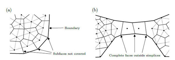
Since we are not making any assumption about the volumes distribution through the mesh, neither about the internal location of its calculation points, then we have to deal with portions of the mesh that are no covered by any simplex. Figure 8 illustrates the two most common cases. The first case takes place in meshes where the calculation points of volumes contiguous to the boundary are in the interior of such volumes, producing subfaces not intersected by any simplex, and the second case occurs when elongated sections of the domain are discretized with a queue of aligned volumes, where each volume has only two neighbors on opposite faces and no simplex can be formed.

Figure 8. (a) When the calculation points of volumes contiguous to the boundary are in the interior of such volumes, there will arise subfaces next to the boundary that can not be covered by any simplex. (b) Portions of the mesh formed by a queue of aligned volumes do not allow the formation of simplices through that queue and there will be whole faces not covered by any simplex

In such cases, the displacement field within the subface ${\textstyle e_{ijk}}$ is a pair-wise polynomial approximation between the adjacent volumes, ${\textstyle \mathbf {x} _{i}}$ and ${\textstyle \mathbf {x} _{j}}$, regardless the dimension

${\boldsymbol {u}}_{ijk}(\mathbf {x} _{g})=\underbrace {\left(1-{P}_{c}\left(z_{g}\right)\right)} _{\varphi _{i}}~{\boldsymbol {u}}_{i}+\underbrace {{P}_{c}\left(z_{g}\right)} _{\varphi _{j}}~{\boldsymbol {u}}_{j},$

(45)

where ${\textstyle \varphi _{i}}$ and ${\textstyle \varphi _{j}}$ are the shape functions, and ${\textstyle z_{g}}$ is the normalized projection of the integration point ${\textstyle \mathbf {x} _{g}}$ into the vector which goes from ${\textstyle \mathbf {x} _{i}}$ to ${\textstyle \mathbf {x} _{j}}$, denoted ${\textstyle \mathbf {x} _{\vec {ij}}=\left(\mathbf {x} _{j}-\mathbf {x} _{i}\right),}$

$z_{g}={\frac {\left(\mathbf {x} _{g}-\mathbf {x} _{i}\right)^{T}\mathbf {x} _{\vec {ij}}}{||\mathbf {x} _{\vec {ij}}||^{2}}}.$

(46)

When calculating the quadrature of equation (26), the pairwise strain is given by

$\left(\mathbf {S} {\boldsymbol {u}}\right)_{ijk}|_{\mathbf {x} _{g}}~~~=\mathbf {S} \varphi _{i}({\boldsymbol {\xi }}_{g})~{\boldsymbol {u}}_{i}~~+~~\mathbf {S} \varphi _{j}({\boldsymbol {\xi }}_{g})~{\boldsymbol {u}}_{j},$ (47) $=\left[{\begin{matrix}\displaystyle {\frac {\partial \varphi _{i}}{\partial \mathbf {x} _{[1]}}}&\\&\displaystyle {\frac {\partial \varphi _{i}}{\partial \mathbf {x} _{[2]}}}\\\displaystyle {\frac {\partial \varphi _{i}}{\partial \mathbf {x} _{[2]}}}&\displaystyle {\frac {\partial \varphi _{i}}{\partial \mathbf {x} _{[1]}}}\end{matrix}}~~~~~{\begin{matrix}\displaystyle {\frac {\partial \varphi _{j}}{\partial \mathbf {x} _{[1]}}}&\\&\displaystyle {\frac {\partial \varphi _{j}}{\partial \mathbf {x} _{[2]}}}\\\displaystyle {\frac {\partial \varphi _{j}}{\partial \mathbf {x} _{[2]}}}&\displaystyle {\frac {\partial \varphi _{j}}{\partial \mathbf {x} _{[1]}}}\end{matrix}}\right]_{|\mathbf {x} _{g}}{\begin{bmatrix}{\boldsymbol {u}}_{i[1]}\\{\boldsymbol {u}}_{i[2]}\\{\boldsymbol {u}}_{j[1]}\\{\boldsymbol {u}}_{j[2]}\end{bmatrix}}$ (48) $=\mathbf {B} _{ijk}|_{\mathbf {x} _{g}}~~~{\vec {\boldsymbol {u}}}_{ijk},$ (49)

In the general case, the gradient is not constant along the face ${\textstyle e_{ij}}$, since its normal is not necessary aligned with ${\textstyle \mathbf {x} _{\vec {ij}}}$, as illustrated in Figure 9.

Figure 9. The gradient of the pairwise approximation is not constant along the face $e_{ij}$, since its normal is not necessary aligned with $\mathbf {x} _{\vec {ij}}$. The integration point is projected into $\mathbf {x} _{\vec {ij}}$ to evaluate the deformation matrix

This pairwise approximation must be used only when necessary because it can not capture the deformation orthogonal to ${\textstyle \mathbf {x} _{\vec {ij}}}$.

3.6 Homeostatic spline

The homeostatic spline is a function of a single variable defined from ${\textstyle z=0}$ to ${\textstyle z=1}$, denoted ${\textstyle {P}_{c}(z)}$, and curved by the parameter ${\textstyle ~c}$, which indicates the level of smoothness. This spline is the simplest polynomial with ${\textstyle ~c~}$ derivatives equal to zero at the endpoints ${\textstyle z=0}$ and ${\textstyle z=1}$. The polynomial degree is given by ${\textstyle 2c+1}$, and such a polynomial requires ${\textstyle N_{g}=c+1}$ integration points to calculate the exact integral in equation (26) using the Gauss-Legendre quadrature.

When designing this spline, we wanted to gain accuracy by building a piece-wise bell-shaped interpolation function around the calculation points, inspired on the infinitely smooth kernels used in other numerical techniques. Therefore, we force the derivatives of the polynomial to be zero over such points in order to homogenize the function. For that reason, we use the term homeostatic spline when referring to this spline.

To fulfill the smoothness requisites commented before, we solved a linear system for calculating the ${\textstyle 2c+2}$ coefficients of the polynomial. The equations of this system were obtained by forcing the ${\textstyle ~c}$ derivatives to be zero at the endpoints. Once we solved the coefficients for the first twenty polynomials, from ${\textstyle c=0}$ to ${\textstyle c=19}$, we found out that the first half of such coefficients are null, and the entire polynomial can be calculated directly as

${P}_{c}(z)={\frac {1}{b_{c}}}\sum \limits _{k=1}^{1+c}(-1)^{k}~b_{k}~~z^{(k+c)},$

(50)

where ${\textstyle b_{k}}$ is the ${\textstyle k^{th}}$ not null coefficient

$b_{k}={\frac {1}{k+c}}\left(\prod \limits _{l=1}^{C_{k}}{\frac {\left(1+c\right)}{l}}-1\right),$

(51)

${\textstyle C_{k}}$ is the number of factors needed to calculate ${\textstyle b_{k}}$

$C_{k}=(c/2)-{\big |}1+(c/2)-k{\big |},$

(52)

and ${\textstyle b_{c}}$ is accumulation of the coefficients for normalizing the spline

$b_{c}=\sum \limits _{k=1}^{1+c}(-1)^{k}b_{k},$

(53)

The first derivative is simply calculated as

${P}_{c}'(z)={\frac {1}{b_{c}}}\sum \limits _{k=1}^{1+c}(-1)^{k}~b_{k}~~(k+c)~~z^{(k+c-1)}$

(54)

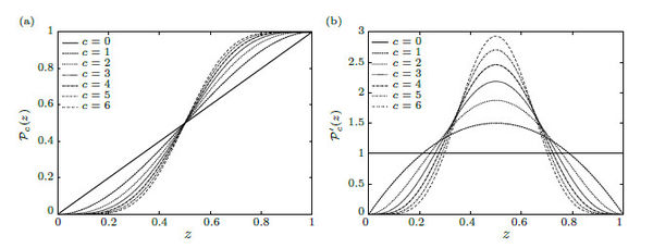
Figure 10(a) shows the evolution of the spline as we increase the smoothness parameter from ${\textstyle c=0}$ to ${\textstyle c=6}$, and Figure 10(b) the evolution of it first derivative. Smoother splines produces higher order polynomials which increases the accuracy of the stress field approximation. This feature is specially important when solving non-linear problems sensibles to the stress field.

Figure 10. (a) The evolution of the homeostatic spline from $c=0$ to $c=6$ illustrates the smoothness requirements at the endpoints of each spline and its (b) first derivatives

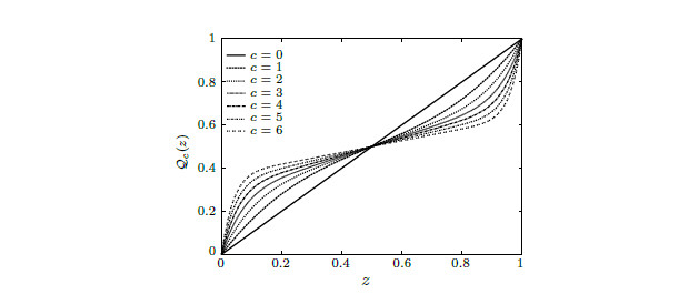
Since the derivatives of the homeostatic spline 50 are zero at the endpoints of the interval ${\textstyle [0,1]}$, the inverse function is not defined in that points. However, we estimate a pseudo-inverse within this interval, ${\textstyle {Q}_{c}\approx {P}_{c}^{-1}}$, by finding the coefficients of a polynomial of the same degree, ${\textstyle 2c+1}$, such that the endpoints coincide with the spline and the first derivative at the midpoint is equivalent to the inverse of the spline first derivative, that is

${Q}_{c}(0)={P}_{c}(0)=0,~~~{Q}_{c}(1)={P}_{c}(1)=1,~~~{\hbox{and}}~~~{Q}_{c}'(0.5)={\frac {1}{{P}_{c}'(0.5)}}$

(55)

The higher derivatives in the midpoint are forced to be zero. Once we calculated the coefficients for the first twenty polynomials, from ${\textstyle c=0}$ to ${\textstyle c=19}$, we found out that the pseudo-inverse can be approximated directly from the following formulae

${Q}(z)=~a_{1}~z~~+~~(a_{1}-1)(2c+1)~\sum \limits _{k=1}^{2c}(-1)^{k}~a_{k}~z^{(k+1)}$

(56)

where ${\textstyle a_{1}}$ is the coefficient for ${\textstyle z}$, and ${\textstyle a_{k}}$ is the factor that distinguish higher order coefficients. Such terms are calculated as

$a_{1}=\left({\frac {c}{2{\sqrt {2}}}}+1\right)^{2},~~~{\hbox{and}}~~~a_{k}=2^{(k-1)}~\prod _{l=1}^{k-1}\left({\frac {2c-l}{2+l}}\right),$

(57)

respectively. Figure 11 exhibits the curves for the first seven levels of smoothness. The null higher derivatives requirement is noticeable at the midpoint.

Figure 11. Curves of the pseudo-inverse ${Q}_{c}$ for the first seven levels of smoothness. The slope at the midpoint exposes the null higher derivatives requirement when increasing the polynomial order

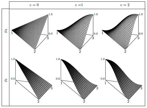
Figure 12 shows the shape functions for the 2D case. The top displays the last node function and the bottom the first node function, the function of the second node is equivalent to that of the first one. The columns separate the first three levels of smoothness. Top and bottom functions coincides at the edges in order to create a continuous field, but only the bottom functions decay uniformly from the node to the opposite edge. The shape functions with ${\textstyle c=0}$ are the only case where all the shape functions are indistinguishable, these are planes.

Figure 12. For the bidimensional case, the top displays the last node function and the bottom the first node function, the function of the second node is equivalent to that of the first one. The columns separate the first three levels of smoothness

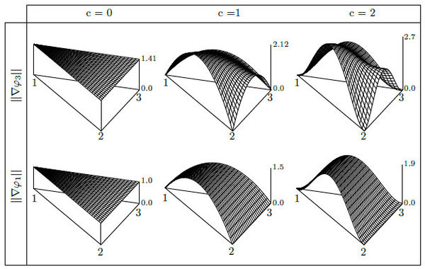
Figure 13 shows the magnitude of the gradient with respect to the normalized space. With the same tabular configuration of Figure 12, the columns separate the first three levels of smoothness, the top displays the last node gradient and the bottom the first node gradient, the gradient of the second node is equivalent to that of the first one. Only the gradient magnitude at the bottom has a uniform variation from the node to the opposite face, and the value of the node does not contribute to the value of such a face. On the contrary, in the top can be observed that the value of the node contributes to the gradient at the opposite face, which means that using ${\textstyle ~c>0~}$ the continuity on the stress field is only guaranteed at the calculation points, but not in the simplices edges.

Figure 13. For the bidimensional case, the top displays the last node gradient magnitudes and the bottom the first node gradient magnitudes, the gradient magnitudes of the second node is equivalent to that of the first one. The columns separate the first three levels of smoothness

3.7 Assembling volume's equation

By using the simplex-wise (42) or the pair-wise (49) approximation, the strain face integral (25) is reformulated as

$\mathbf {H} _{ij}=\sum \limits _{k=1}^{N_{ij}}\sum \limits _{g=1}^{N_{g}}~~w_{g}~\mathbf {B} _{ijk}|_{\mathbf {x} _{g}}~{\vec {\boldsymbol {u}}}_{ijk},$

(58)

then, the volume equilibrium equation (22) is

$\sum \limits _{j=1}^{N_{i}}\mathbf {T} _{ij}\mathbf {D} _{ij}\sum \limits _{k=1}^{N_{ij}}\sum \limits _{g=1}^{N_{g}}~~w_{g}~\mathbf {B} _{ijk}|_{\mathbf {x} _{g}}~{\vec {\boldsymbol {u}}}_{ijk}=0,$

(59)

reordering the terms we obtain

$\sum \limits _{j=1}^{N_{i}}\sum \limits _{k=1}^{N_{ij}}\sum \limits _{g=1}^{N_{g}}~~w_{g}~\mathbf {K} _{ijk}|_{\mathbf {x} _{g}}~{\vec {\boldsymbol {u}}}_{ijk}=0,$

(60)

where the matrix

$\mathbf {K} _{ijk}|_{\mathbf {x} _{g}}=\mathbf {T} _{ij}\mathbf {D} _{ij}\mathbf {B} _{ijk}|_{\mathbf {x} _{g}},$

(61)

is the stiffness contribution at the integration point ${\textstyle \mathbf {x} _{g}}$, within the subface ${\textstyle e_{ijk}}$ when integrating the ${\textstyle i^{th}}$ volume. Observe that the stiffness matrix ${\textstyle \mathbf {K} _{ijk}}$ is rectangular and the resulting global stiffness matrix is asymmetric.

3.8 Boundary conditions

The Neumann boundary conditions are imposed over the volume faces ${\textstyle e_{ij}}$ intersecting the boundary, by replacing the corresponding term in the sum of equation (20) with the integral of the function provided in (6.a),

$\int _{e_{ij}}\mathbf {T} \mathbf {D} \mathbf {S} {\boldsymbol {u}}~dS=\int _{e_{ij}}{\boldsymbol {b}}_{N}(\mathbf {x} )~dS$

(62)

The Dirichlet conditions are imposed over the volumes calculation points by fixing the displacement as it is evaluated in the function given in (6.b),

${\boldsymbol {u}}_{i}={\boldsymbol {u}}_{D}(\mathbf {x} _{i}),$

(63)

Since the Dirichlet conditions are imposed directly on the calculation points, these points must be located along the face ${\textstyle e_{ij}}$ which intersects the boundary with the condition ${\textstyle \Gamma _{D}}$.

3.9 Special cases

By making some considerations, we identify two special cases where the calculations can be simplified, in order to increase the performance of the total computation, at the expense of losing control over the volumes shape. These cases are: 1) the Voronoi mesh assumption and 2) the FV-FEM correlation.

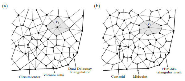
In the first case, we assume that the initial mesh is equivalent to the Voronoi diagram and that the Voronoi centres correspond to the calculation points ${\textstyle \mathbf {x} _{i}}$. Hence, the subdivision of the neighborhood ${\textstyle {B}_{i}}$ is already given by the Delaunay triangulation which is dual to the Voronoi mesh, as illustrated in Figure 14(a). Moreover, the integrals of subfaces ${\textstyle e_{ijk}}$ using pair-wise approximations can be exactly integrated with the midpoint rule, since the faces are orthogonal to the vector joining the calculation points ${\textstyle \mathbf {x} _{\vec {ij}}}$, and the derivatives along the subface are constants.

Figure 14. (a) The initial mesh is equivalent to the Voronoi diagram and the Voronoi centres correspond to the calculation points $\mathbf {x} _{i}$. (b) The initial mesh is generated from a FEM-like triangular mesh. The calculation points $\mathbf {x} _{i}$ are defined to be the nodes of the triangular mesh, and the volume faces are created by joining the centroids of the triangles with the midpoint of the segments

In the second case, the initial mesh is generated from a FEM-like triangular mesh and the approximations are assumed to be linear. In such a case, the calculation points ${\textstyle \mathbf {x} _{i}}$ are defined to be the nodes of the triangular mesh, and the volume faces are created by joining the centroids of the triangles with the midpoint of the segments, as presented in Figure 14(b). This particular version is equivalent to the cell-centred finite volume scheme introduced by Oñate et al. [7], who proved that the global linear system produced by this FV scheme is identical to that produced by FEM if the same mesh is used.

4. Results

In order to test the numerical performance of the proposed method, we use the well known analytical experiment of an infinite plate with a circular hole in the origin [26]. In such a experiment, the plate is stretched along the horizontal axis with a uniform tension of ${\textstyle \mathbf {f} _{[1]}=10~~kPa}$ from each side, as is shown in Figure 15. The material is characterized by the Poisson ratio, ${\textstyle \nu =0.3}$, and Young modulus, ${\textstyle E=10~~MPa}$. Plane stress is assumed with thickness equivalent to the unity. The dimensions of the computational domain are ${\textstyle a=0.5m}$ and ${\textstyle b=2m}$.

Figure 15. (a) Infinite plate with a hole being stretched along the horizontal axis with a force of $\mathbf {f} _{[1]}=10~~kPa$ from each side. (b) Computational domain, $a=0.5m$ and $b=2m$, with axysymmetrical assumptions used to test the numerical method. The polar coordinates, $r$ and $\theta$, for calculating the analytical stress field

The analytical solution is given by the following formulae

${\boldsymbol {\sigma }}_{[11]}=\mathbf {f} _{[1]}\left[1-{\frac {a^{2}}{r^{2}}}\left({\frac {3}{2}}\cos(2\theta )+\cos(4\theta )\right)+{\frac {3a^{4}}{2r^{4}}}\cos(4\theta )\right],$ (64) ${\boldsymbol {\sigma }}_{[22]}=\mathbf {f} _{[1]}\left[-{\frac {a^{2}}{r^{2}}}\left({\frac {1}{2}}\cos(2\theta )-\cos(4\theta )\right)-{\frac {3a^{4}}{2r^{4}}}\cos(4\theta )\right],$ (65) ${\boldsymbol {\sigma }}_{[12]}=\mathbf {f} _{[1]}\left[-{\frac {a^{2}}{r^{2}}}\left({\frac {1}{2}}\sin(2\theta )+\sin(4\theta )\right)+{\frac {3a^{4}}{2r^{4}}}\sin(4\theta )\right],$ (66)

where the polar coordinates,

$r={\sqrt {\mathbf {x} _{[1]}^{2}+\mathbf {x} _{[2]}^{2}}},~~~{\hbox{and}}~~~\theta =\tan ^{-1}\left({\frac {\mathbf {x} _{[2]}}{\mathbf {x} _{[1]}}}\right),$

(67)

are used within the calculus. Figure 16(a) exhibits the discretization of the computational domain into 2411 polygonal volumes used to compare the numerical results against the analytical stress field. This mesh is not equivalent to the Voronoi diagram; Figure 16(b) the level sets of ${\textstyle {\boldsymbol {\sigma }}_{[11]}}$ between ${\textstyle 0}$ to ${\textstyle 30~~kPa}$, with steps of ${\textstyle 1~~kPa}$. Figure 16(c) Level sets of ${\textstyle {\boldsymbol {\sigma }}_{[22]}}$ between ${\textstyle -10}$ and ${\textstyle 6~~kPa}$, with steps of ${\textstyle 0.8~~kPa}$ and Figure 16(d) Level sets of ${\textstyle {\boldsymbol {\sigma }}_{[12]}}$ between ${\textstyle -10}$ and ${\textstyle 2~~kPa}$, with steps of ${\textstyle 0.6~~kPa}$.

Figure 16. (a) Polygonal mesh used for comparison of numerical results. (b) Level sets of ${\boldsymbol {\sigma }}_{[11]}$ between $0$ to $30~~kPa$. (c) Level sets of ${\boldsymbol {\sigma }}_{[22]}$ between $-10$ and $6~~kPa$. (d) Level sets of ${\boldsymbol {\sigma }}_{[12]}$ between $-10$ and $2~~kPa$

The Dirichlet conditions are imposed on the bottom and left side of the computational domain as is shown in Figure 16(b). Next in order, the analytic stress of equations (64), (65) and (66) is imposed as Neumann condition over the top and right side of the computational domain.

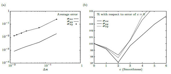
Figure 17(a) presents the averaged error as a function of the volumes face length mean, denoted ${\textstyle \Delta x}$, as we might expect, the error is proportional to the mesh refinement. For a mesh of 478 volumes, Figure 17(b) shows the percentage of the error with respect to the error of ${\textstyle c=0}$, for different smoothing levels, ${\textstyle c=0}$ correspond the linear interpolator. Observe that the error of the stress field does not decreases significantly because we do not increase the degrees of freedom of the linear system, although we built a better field description, which can be useful when solving non-linear formulations.

Figure 17. (a) The averaged error decreasing as a function of mesh size, denoted $\Delta \mathbf {x}$. (b) Using a mesh of 628 volumes, percentage of error for different smoothing levels with respect to the error of $c=0$, which is the linear interpolator, error increases after $c=2$

5. Conclusions

In this work we discussed a numerical technique to solve the elasticity equation for unstructured and non conforming meshes formed by elements of any arbitrary polygonal/polyhedral shape. The elasticity-solver is based on a finite volume formulation that, using the divergence theorem, represent the volume integral of the stress divergence in terms of the surface integral of the stress over the volume boundary. For considering the unit vector normal to the boundary as a constant, the boundary is divided into flat faces. Conforming and non-conforming meshes are processed without distinction. The displacement field is a piece-wise polynomial approximation surrounding the volumes, built on the top of the simplices resulting from the Delaunay triangulation of the volume neighborhood. A pair-wise polynomial interpolation is used for neighborhoods where the simplices are not the best option, and for 1D problems.

We introduced the homeostatic splines and it pseudo-inverse for higher order polynomial interpolations without the necessity of increasing the discretization points.

Since the stress term is calculated directly on the boundary of the control volumes, this strategy can be used in fracture formulations where the volumes are treated as indivisible components and the rupture occurs across the volumes boundaries.

In future work, we will investigate the accuracy of this numerical procedure for solving non-linear and dynamic models when using higher order homeostatic splines.

Acknowledgement

The present investigation was sponsored by a CONACYT scolarship from the Mexican government and the TCAiNMaND project, an IRSES Marie Curie initiative under the European Union 7th Framework Programme. In addition, the authors want to express his gratitude to MSc. Ernesto Ortega, and to Drs. Rafel Herrera and Joaquin Peña for his insightful commments and discussions during the elaboration of this paper.

References

[1] Slone A.K., Pericleous K., Bailey C., Cross M. Dynamic fluid-structure interaction using finite volume unstructured mesh procedures. Computers and Structures, 80:371-390, 2002.

[2] Slone A.K., Pericleous K., Bailey C., Cross M., Bennett C. A finite volume unstructured mesh approach to dynamic fluid-structure interaction: an assessment of the challenge of predicting the onset flutter. Applied Mathematical Modeling, 28:211-239, 2004.

[3] Bailey C., Taylor G.A., Cross M., Chow P. Discretisation procedures for multi-physics phenomena. Journal of Computational and Applied Mathematics, 103:3-17, 1999.

[4] Souli M., Ouahsine A., Lewin L. ALE formulation for fluid-structure interaction problems. Computer Methods in Applied Mechanics and Engineering, 190:659-675, 2000.

[5] Lubliner J., Oliver J., Oller S., Oñate E. A Plastic-Damage model for concrete. International Journal of Solids and Structures, 25:299-326, 1989.

[6] Armero F., Oller S. A general framework for continuum damage models. I. Infinitesimal plastic damage models in stress space. International Journal of Solids and Structures, 37:7409-7436, 2000.

[7] Oñate E., Cervera M., Zienkiewicz O.C. A finite volume format for structural mechanics. International Journal for Numerical Methods in Engineering, 37:181-201, 1994.

[8] Idelsohn S.R., Oñate E. Finite volumes and finite elements: Two 'Good Friends'. International Journal for Numerical Methods in Engineering, 37:3323-3341, 1994.

[9] Fryer Y.D., Bailey C., Cross M., Lai C.H. A control volume procedure for solving the elastic stress-strain equations on an unstructured mesh. Applied Mathematical Modeling, 15:639-645, 1991.

[10] Bailey C., Cross M. A Finite Volume procedure to solve elastic solid mechanics problems in three dimensions on an unstructured mesh. International Journal for Numerical Methods in Engineering, 38:1757-1776, 1995.

[11] Slone A.K., Bailey C., Cross M. Dynamic solid mechanics using finite volume methods. Applied Mathematical Modeling, 27(2):69-87, 2003.

[12] Demirdzic I., Martinovic D. Finite volume method for thermo-elasto-plastic stress analysis. Computer Methods in Applied Mechanics and Engineering, 109:331-349, 1993.

[13] Demirdzic I., Muzaferija S. Finite volume methods for stress analysis in complex domains. International Journal for Numerical Methods in Engineering, 137:3751-3766, 1994.

[14] Demirdzic I., Muzaferija S., Peric M. Benchmark solutions of some structural analysis problems using finite-volume method and multigrid acceleration. International Journal for Numerical Methods in Engineering, 40:1893-1908, 1997.

[15] Bijelonja I., Demirdzic I., Muzaferija S. A finite volume method for large strain analysis of incompressible hyperelastic materials. International Journal for Numerical Methods in Engineering, 64:1594-1609, 2005.

[16] Bijelonja I., Demirdzic I., Muzaferija S. A finite volume method for incompressible linear elasticity. Computer Methods in Applied Mechanics and Engineering, 195:6378-6390, 2006.

[17] Jasak H., Weller H.G. Application of the finite volume method and unstructured meshes to linear elasticity. International Journal for Numerical Methods in Engineering, 48:267-287, 2000.

[18] Tukovic Z., Ivankovic A., Karac A. Finite-volume stress analysis in multi-material linear elastic body. International Journal for Numerical Methods in Engineering, 93(4):400-419, 2012.

[19] Tang T., Hededal O., Cardiff P. On finite volume method implementation of poro-elasto-plasticity soil model. International Journal for Numerical and Analytical Methods in Geomecanics, 39:1410-1430, 2015.

[20] Borden M.J., Verhoosel C.V., Scott M., Hughes T.J.R., Landis C.M. A phase-field description of dynamic brittle fracture. Computer Methods in Applied Mechanics and Engineering, 217-220:77-95, 2012.

[21] Cardiff P., Tukovic Z., Jasak H., Ivankovic A. A block-coupled Finite Volume methodology for linear elasticity and unstructured meshes. Computers and Structures, 175:100-122, 2016.

[22] Cavalcante M.A.A., Pindera M-J. Generalized Finite-Volume Theory for Elastic Stress Analysis in Solid Mechanics - Part I: Framework. Journal of Applied Mechanics, 79(5):1006-1017, 2012.

[23] Nordbotten J.M. Cell-centered finite volume discretizations for deformable porous media. International Journal for Numerical Methods in Engineering, 100:399-418, 2014.

[24] Li B., Chen Z., Huan G. Control volume function approximation methods and their applications to modeling porous media flow. Advances in Water Resources, 26(4):435-444, 2003.

[25] Li B., Chen Z., Huan G. Control volume function approximation methods and their applications to modeling porous media flow II: the black oil model. Advances in Water Resources, 27(2):99-120, 2004.

[26] Timoshenko S.P., Goodier J.N. Theory of Elasticity. McGraw-Hill, 3 Edition, 1970.