Determination of specific heat capacity by transient plane source

Abstract

A standard TPS measurement gives the thermal conductivity and thermal diffusivity of an isotropic material which in turn gives the heat capacity. The thermal properties of an anisotropic material can be measured if the heat capacity is known. A method for heat capacity measurement exists, where the TPS sensor is attached to a sample container which is surrounded by insulation. However, its based on an assumption of negligible heat losses which leads to uncertainties in the results. From that position, this work aims to model the heat losses from the specific heat measurements with TPS. A new set-up is introduced, where the sensor with the container hangs freely in a steel tube to get more predictable heat losses.

 The results show that the measurements can be modelled as a network of lumps connected by conductances approximated as constant. Thereby, the conductances out from the system can be solved from a reference measurement and used as input for a model of a measurement with a sample. The model seems to underestimate the heat capacity, which might be a consequence of temperature dependent effects on the conductances from convection. The tube in the set-up could be evacuated to minimize those losses.

Keywords

Specific heat capacity ; Transient plane source ; TPS

1. Introduction

Specific heat capacity of materials and components are of vital importance in their final functionality i.e. thermal storage in building elements or transient heat flux.

There are different methods for determination of the specific heat capacity. One method is the adiabatic calorimetry where heat is added to a sample while the temperature increase is measured continuously. The sample is surrounded by a heating guard keeping the initial measuring temperature to minimize the heat losses from the sample to the surrounding. If the losses are negligible, the heat capacity can be calculated from the known energy input and temperature by Eq. (1) .

$mc_{p}={\frac {\Delta E}{\Delta T}}={\frac {{\int }_{t1}^{t2}Pdt}{\Delta T}}$

( 1)

where m is the mass (kg), c_p is the specific heat capacity (J/kg/K), E is the heating energy (J), ΔT is the temperature change (K), P is the power input (W), t is the time (s).

Matsou (1988) describes that the adiabatic method works best at lower temperatures where almost adiabatic condition can be reached and thus is a good estimate for the heat capacity calculations. At higher temperatures the heat losses has to be taken into account or they will influence the calculated results. Karasz and O'Reilly (1966) solve the problem with adiabatic conditions by letting the heating guard follow the temperature increase of the sample.

The TPS method (ISO 22007-2, 2008 ) can be used for simultaneous determination of thermal conductivity, thermal diffusivity and specific heat of an isotropic material. To measure the thermal properties of anisotropic material, the specific heat capacity has to be known. This creates an incentive to create a model for measuring the specific heat capacity with the TPS equipment.

In this paper, the specific heat capacity has been measured by a TPS-sensor. The method is similar to the adiabatic method but does not assume adiabatic conditions. Matsou (1988) created an extrapolation method to quantify the heat losses from the cooling of the sample. The heat losses to the surroundings could instead be incorporated in the model for heat capacity calculation, which has been examined in this paper.

2. Principle of transient plane source

Gustafsson et al. (1979) Chalmers University of Technology, Sweden, first demonstrated the TPS principle. The TPS method uses a sensor which is a combined heat source and resistance thermometer. A constant power is supplied to the sensor and the temperature in the sensor is continuously measured. The thermal properties of the sample can be calculated by using the temperature development in the sensor. A TPS sensor is shown in Figure 1 .

Figure 1. Picture of a TPS sensor.

2.1. Existing method to measure of heat capacity with TPS

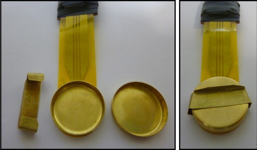
Determination of the specific heat capacity can be performed by the measurement procedure described in the Hot Disk (2001 ) manual. In specific heat application a TPS sensor is attached to the underside of a gold container (sample holder), shown in Figure 2 . The container limits the size of the sample which for this case is a cylinder with a diameter of 20 mm and a height of 5 mm.

Figure 2. Gold container glued to a TPS sensor for specific heat measurements. The open container to the left and the closed container ready for measurement to the right.

The process of measuring is based on two individual measurements; a reference measurement (the empty container) and a sample measurement (the container withholding a sample). In order to minimize the heat losses to ambient air, in both measurements the setup of the sensor, holder and sample are imbedded in a low conductive material.

The method is based on the assumption of a linear temperature increase (Gustavsson et al., 1996 ), which would mean that the heat losses to the surroundings are negligible for the time span of the measurement. The heat capacity would be calculated by Eq. (1) as for the adiabatic calorimetry.

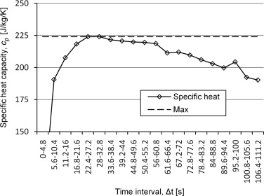
To find the right time span for the analysis, the measurement data could be analysed in a variety of time windows. The results will give a curve with a maximum that is close to the specific heat of the analysed material. An example of the results is shown in Figure 3 .

Figure 3. Analyses of measuring points for determination of specific heat with a silver sample with specific heat of 235 J/kg/K.

The method is time consuming and there is a problem with the reliability of the results. If the later decrease of the curve comes from the losses that start to influence the measurement, there will always be a risk that the losses start to have an influence already before the plateau which would make the model underestimate the specific heat. It will also be hard to choose an adequate time interval for the analysis.

2.2. Comparison of different set-ups

To test the influence of the losses, and to connect them to heat transfer mechanisms, three different set-ups for the mounting of the gold container have been tested for measuring the heat capacity with TPS:

• The old set-up where the sample container and the sensor were put in a hole between two blocks of XPS insulation.
• The sample container hanging inside a steel tube at atmospheric pressure.
• The sample container hanging inside a steel tube at 10 kPa pressure.

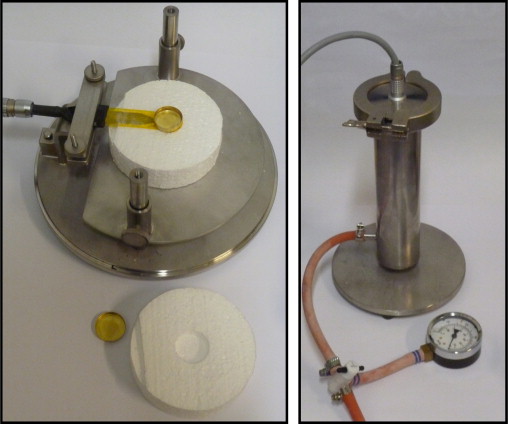
The devices for the different set-ups are shown in Figure 4 where the same steel tube is used for both set-up 2 and 3. A fan was used for evacuating the tube in set-up 3 which reached down to a pressure of 10 kPa. The sensor is either placed in the insulation or freely hanged in its leads from the lid of the tube.

Figure 4. The device used for set-up 1 is shown to the left and the device used for set-up 2 and 3 to the right.

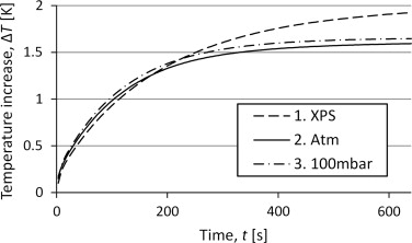
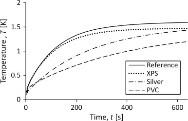
To compare the different set-ups, and chose which to study further, measurements were made with the empty container. Figure 5 shows the corresponding temperature curve for the three different set-ups. For all three measurements, a power of 10 mW has been supplied for 640 s. The temperature seems to increase asymptotically toward a stable temperature where the heat losses will balance the power input. The curves stabilize at different temperatures which means that the losses vary between the different set-ups. Set-up 1 with XPS seems to have considerably lower amounts of losses while the change in pressure conditions seems to have a quite small effect.

Figure 5. Curves for the temperature increase for reference measurements with the three different set-ups.

The results presented in Figure 4 indicate that the deviation between set-up 2 and 3 can be neglected, thus it is unnecessary to evacuate the tube. The main influence from a lowered pressure would be on the convection since the radiation is independent on pressure and a pressure of 10 kPa is too high to influence the conduction in such a large cavity. This suggests that the convection plays a minor part in the heat losses. That gives better possibilities to develop a mathematical model of the temperature increase since both the radiation flux and the conduction flux can be considered linearly dependent of temperature at these temperature intervals, while the conduction would have been dependent on higher degrees of the temperature difference.

For the case with insulation around the sensor there might appear both some transient behavior of the heat waves expansion through the insulation material and, after a certain time of the measurement, effects from the boundaries of the insulation.

For the case with the steel tube, the large inner area, high heat capacity and high conductivity will lead to a negligible temperature increase in the tube for the magnitude of the power and times used in these experiments. Thus, assuming a constant temperature boundary condition is a good approximation. This will although be a limitation for the possible time over which the model would be valid for that set-up.

Thereof the set-up 2 with the steel tube at atmospheric pressure will be the focus of this paper and will be used for both simulations and measurements in further chapters.

3. Analysis of transient measurements

The heat capacity should be possible to calculate by using the measured temperature increase since it seems to govern the shape of the curve. This can be seen in Figure 6 which shows the curves for the empty container and measurements on three different sample materials with varying heat capacity. A higher heat capacity will lead to a slower incline of the temperature. This correspond to Figure 6 since mc_{p XPS} <mc_{p silver} <mc_{p PVC} . Approximate properties of the materials are shown in Table 1 . The mass of PVC is large compared to that of silver because the silver sample is a folded foil and thus not as compact as a homogenous material.

Figure 6. Temperature development in the sensor for measurements on samples of materials with varying specific heat capacity.

Table 1. Approximate values of heat capacity for some sample materials.

Material	Sample mass (g)	Specific heat capacity (J/g/K)	Heat capacity (J/K)
XPS	0.042	0.8	0.034
Silver	4.2	0.24	1.0
PVC	2.2	0.8	1.8

3.1. One lump model

The simplest mathematical model would be that the whole sample container with the sample behaves as an isothermal lump. When a heat source is connected to the lump, the energy from the source will either heat up the lump or be transported away from the lump as losses. This system is illustrated in Figure 7 where the temperature T (t ) is the temperature difference measured by the TPS device.

Figure 7. Model for the heat capacity measurement with TPS.

The model in Figure 7 leads to the heat transfer equation shown in Eq. (2) which describes that the change of energy in the lump (sample and container) is the difference between the power added to the system and the energy loss from the system:

$mc_{p}{\frac {\partial T}{\partial t}}=P-K(T)\times T(t)$

( 2)

where m is the mass (kg), c_p is the heat capacity (J/kg/K), T is the temperature (K), t is the time (s), P is the power input (W) and K (T ) is the conductance to the surroundings (W/K).

If the conductance, K , is constant (not dependent of temperature), Eq. (2) can be solved analytically with the results shown in Eq. (3) together with Eq. 4 ):

$T(t)={\frac {P}{K}}(1-e^{-t/t_{c}})$

( 3)

$t_{c}={\frac {mc_{p}}{K}}$

( 4)

where t_c is the time constant (s).

The behavior of Eq. (3) can be seen in Figure 5 where the curves seem to stabilize at some specific temperature which would equal the quotient P/K . Eq. (3) would give similar curves for measurements of the container with a sample. The sample measurement would have a slower ascent toward the steady state temperature due to a higher time constant when the value for mc_p is increased in Eq. (4) . This can be seen in Figure 6 .

3.2. Two lump model

To analyze the assumption of a lumped model representing the true characteristics of the of the set-up, an analysis were done of a more complex mathematical model shown in Figure 8 . Here, the side of the container where the sensor is placed is separated from the other side by an internal conductance and the power source is connected only to the sensor side.

Figure 8. Schematics of the model used for simulations. The container is separated into two lumps with an internal conductance, Kint , connecting them together and both connected to the exterior with Kext .

With this model it is possible to analyze the consequence of getting all your data from a single side of the specimen. For this symmetrical case, where the heat capacity is the same for both nodes and the conductance are the same in both directions, the temperatures in the model could be calculated analytically by Eq. (5) together with Eq. (6) and Eq. (7) :

$\lbrace {\begin{array}{c}T_{1}(t)=T_{s1}-{\frac {T_{s1}+T_{s2}}{2}}e^{-t/t_{c}}-{\frac {T_{s1}-T_{s2}}{2}}e^{-t/{t{'}}_{c}}\\T_{2}(t)=T_{s2}-{\frac {T_{s1}+T_{s2}}{2}}e^{-t/t_{c}}+{\frac {T_{s1}-T_{s2}}{2}}e^{-t/{t{'}}_{c}}\end{array}}$

( 5)

$t_{c}={\frac {mc_{p}}{2K_{ext}}}$

( 6)

${t{'}}_{c}={\frac {mc_{p}}{2(K_{ext}+2K_{int})}}$

( 7)

where T_{s 1} and T_{s 2} are the steady state temperatures at corresponding node (K ), t_c and t_c ' is time constants (s ), K_ext is the conductances to the exterior (W/K) and K_int is the conductance from one side of the container to the other (W/K).

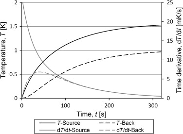
The temperatures in Eq. (5) were calculated from input based on heat transfer through radiation and conduction for set-up 2, with the steel tube at atmospheric pressure. The results are shown in Figure 9 . Both the temperature increase and its time derivative are shown for both the front side (source side) and the back side of the container. It is interesting to see that the derivatives seems to come together and follow the same curve which means that from this point the equation for the two temperature curves are the same, but for a constant. This can also be seen in Eq. (5 ) for the case where K_int is large compared to K_ext . The third term in the equation will decline faster than the second term which is the same for both temperatures. After long enough time for the third term to be negligible, the equation for the sensor temperature can be rearranged to Eq. (8) , which is the same as Eq. (3) apart from the constant (T_{s 1} −T_{s 2} )/ 2. This makes it into an equation with three unknowns of which one, the constant, does not contribute to the solution of the heat capacity.

$T_{1}(t)={\frac {T_{s1}-T_{s2}}{2}}-{\frac {P}{2\times K_{ext}}}(1-$$e^{-t/t_{c}})$

( 8)

Figure 9. The figure shows the analytical solution for the two sides of the container. The input data is based on measurements of the empty container. After 100 s the time derivatives coincide.

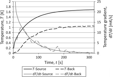
Validation of the calculated results was performed by measuring the temperature the temperature of the backside of the container, shown in Figure 10 . The behavior of the curves from the measurements looks very close to that of the analytical solution.

Figure 10. Results from measurements with a TPS sensor on one side of the container and a thermocouple on the other side.

3.3. Three lump model

The previous results, showed in Figure 9 and Figure 10 , are for the empty container. If a sample is added, the symmetry of the system will disappear. For this case a three lump model, shown in Figure 11 , were analyzed.

Figure 11. Schematics of the three lump model. A lump with a varying heat capacity, for example a sample, is added to the system.

If the assumptions in those models, the two lump model for the empty container and the three lump model for the container with a sample, are valid, then mc_{p 1} and K_ext should be the same in both models. To test that, Eq. (8) can be fitted to the temperature curve of a reference measurement with the empty container. That gives the external conductance and the heat capacity of the holder. Then there are only two unknown variables left in the three lump model; mc_{p 2} and K ′_int .

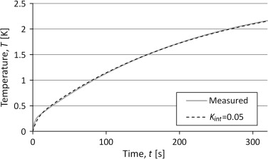
The temperatures in the three lump model were solved numerically with input data from the curve fit of the two lump model. The heat capacity of the sample was set to the heat capacity pure silver, 235 J/kg/K, and the internal conductance was adjusted to fit a measurement with a sample of pure silver.

The results are shown in Figure 12 where the internal conductance, K_int , of 0.05 W/K gives a very good result. This suggests that the external conductance is the same, both for the reference measurement and the sample measurement.

Figure 12. Results from simulations of the three lump model with input data from the two lump model and heat capacity from material data for pure silver. The results are compared to measured temperatures for a silver sample.

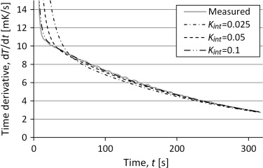
To analyze the sensitivity of the variation in heat capacity and internal conductance the, simulations were made with a variation of the input data. The result for the time derivatives for variation of internal conductance is shown in Figure 13 . There is an influence on the shape of the temperature curve from the internal conductance but the variation is quite small.

Figure 13. Time derivative of the temperature from simulations of the three lump model with varying internal conductance. Compared to measurements of a silver sample.

To make a first test of the possibility to predict the heat capacity with the models, simulations were made for a variation of heat capacity and internal conductance. The simulation results were fit to the absolute temperature difference and its time derivative from measurements of a silver sample. The specific heat and the internal conductance which gave the lowest quadratic distance are shown in Table 2 .

Table 2. Results from simulations over a variation of specific heat and internal conductance. The value is taken for the simulation which gave the least squared distance between the simulated temperature curve and a measured curve.

Analysed curve	Specific heat capacity (J/kg/K)	Internal conductance (J/K)	Error from tabulated value⁎ (%)
T (t )	218	0.052	−7.2
dT (t )/dt	221	0.051	−6.0

⁎. Tabulated value for pure silver is 235 J/kg/K.

The results are similar between both curves which suggest that the temperature and its time derivative contain the same information. Both analyses underestimate the heat capacity compared to the tabulated value for silver.

4. Conclusions and discussion

It seems as if the set-up with the sensor hanging in a steel tube is the easiest one to model, relative to set-up with insulation. There were small differences between low pressure measurements and measurements at atmospheric pressure why the analysis was made for atmospheric pressure.

From the analysis of the heat losses, the two lump model gives a good estimate of the measurements for the case with an empty container. In addition, the analytical solution show that it might take some while before the one sided measurement represents the mean temperature development. This means that the model needs to come with good recommendations on which part of the measurement to use in the analysis.

The conductance and heat capacity calculated from the reference measurement can be used as input data for the three lump model, which gave good results compared to the measurement of a sample with known heat capacity.

When the model were simulated for a variation of heat capacities and internal conductances and compared to a measured curve with the least square method, the resulting heat capacity underestimated the table value.

The underestimation can be a consequence of a temperature dependence of the conductance. If the external conductance increases with temperature, the temperature would increase faster in the beginning and slower at the end. With a model assuming constant conductances this would be interpreted as a lower heat capacity, which is what has been obtained. This suggests that the convection might influence the results and cannot be neglected as has been assumed. The set-up with vacuum will decrease the convection which is seen in Figure 5 as the difference between vacuum and atmospheric pressure. This makes the vacuum set-up interesting for further studies.

The error in the heat capacity could also come from the simplifications in the models where some heat transfer paths are neglected. If the evacuated measurements do not give better results the models might have to be more advanced.

In this report the method has mainly been tested for a silver sample, a material with high volumetric heat capacity and high thermal conductivity. The model also has to be tested for materials with different thermal properties to see if the results are common.

Acknowledgements

This work has been funded by Fjärrvärmeföreningen through the project “Högpresterande fjärrvärmerör” and by the EU-project “FC-district” which is gratefully acknowledged. Also a great thank to Silas Gustafsson for valuable input.

References

1. Gustavsson et al., 1996 M. Gustavsson, N.S. Saxena, E. Karawacki, S.E. Gustafsson; Specific heat measurements with the hot disk thermal analyser; Thermal Conductivity, 23 (1996), pp. 56–65
2. Gustafsson et al., 1979 S.E. Gustafsson, E. Karawacki, M.N. Khan; Transient hot-strip method for simultaneously measuring thermal conductivity and thermal diffusivity of solids and fluids; Journal of Physics D: Applied Physics, 12 (1979), pp. 1411–1421
3. Disk, 2001 Hot Disk. 2001. Instruction Manual: Hot disk Thermal Constants analyser Windows 95/98 Version 5.0
4. ISO 22007-2, 2008 ISO 22007-2. 2008. Plastics-Determination of Thermal Conductivity and Thermal Diffusivity—Part 2: Transient Plane Heat Source (Hot Disc) Method.
5. Karasz and O'Reilly, 1966 F.E. Karasz, J.M. O'Reilly; Wide temperature range adiabatic calorimetry; The Review of Scientific Instruments, 37 (3) (1966), pp. 255–260
6. Matsou, 1988 S. Matsou; Correction methods for heat leaks in adiabatic calorimetry; Thermochimica Acta, 125 (1988), pp. 307–318