A fractional numerical study on a plant disease model with replanting and preventive treatment

Abstract

Food security has become a significant issue due to the growing human population. In this case, a significant role is played by agriculture. The essential foods are obtained mainly from plants. Plant diseases can, however, decrease both food production and its quality. Therefore, it is substantial to comprehend the dynamics of plant diseases as they can provide insightful information about the dispersal of plant diseases. In order to investigate the dynamics of plant disease and analyze the effects of strategies of disease control, a mathematical model can be applied. We show that this model provides the non-negative solutions that population dynamics requires. The model was investigated by using the Atangana-Baleanu in Caputo sense (ABC) operator which is symmetrical to the Caputo-Fabrizio (CF) operator with a different function. Whereas the ABC operator uses the generalized Mittag-Leffler function while the CF operator employs the exponential kernel. For the proposed model, we have displayed the local and global stability of a nonendemic and an endemic equilibrium, existence and uniqueness theorems. By applying the fractional Adams-Bashforth-Moulton method, we have implemented numerical solutions to illustrate the theoretical analysis.

Keywords: Adams-Bashforth-Moulton method, local and global asymptotic equilibrium stability, sensitivity analysis, existence theorems, uniqueness theorems, plant diseases model, numerical simulations

1. Introduction

Plants are an incredibly valuable component of our world. The earth, due to the presence of plants, is known as a green planet. They are perhaps the most important component of the life of all the earth's living beings. Some of the plant's essential functions are food, reducing the level of pollution, supplying fresh oxygen, medications, furniture and refuge. Plant disease, however, triggers a decline in food production and efficiency, which can lead to numerous health and social issues. Moreover, it can cause considerable economic ramifications.

Plant disease epidemiology studies the evolution of populations of plant diseases in time and space. Usually, the execution of the techniques is accomplished by roguing and then replanting, which offers two possible advantages. Initially, infected plants could be removed and could inoculum sources could be reduced, possibly slowing the dispersal of pathogens. Then, the infected plant may die or suffer a reduction in yield. Consequently, substituting diseased plants with healthful plants can indemnity crop casualties. The exposed plant can also be able to spread disease in some cases [1-3]. Since the exposed plant is capable of spreading disease, the propagation of plant disease can be more rapid. It is therefore important to realize the impact of plants uncovered on the dynamics of plant disease contamination. Their simulation revealed that the application of fungicides is efficient in minimizing population infection [4-6].

Mathematical modeling is useful in explaining how diseases dispersal and different factors involved in the dispersal of the disease have been specified [7-11]. The defensive and curative fungicide model was introduced in Anggriani et al. [12], where it has been split into three ingredients: Infectious, protected and susceptible. Their simulation revealed that the implementation of fungicides is active in minimizing population infection. Model plant diseases with replanting, roguing and preventive care have been introduced in Anggriani et al. [13] without consideration to curative therapy. In 2017, Anggriani et al. [14] created a plant disease mathematical model that includes five ingredients: Susceptible, Protected, Infectious, Exposed and Post-Infectious with protective curative therapies. They observed that by using curative and preventative care, the transmission of plant disease can be minimized. However, where only one therapy is offered, preventive therapy is favored over curative therapy.

In actuality, there are various meanings of fractional derivatives which in general do not necessarily correspond. One of these definitions which is often utilized in different implementations of fractional differential equations is Caputo fractional derivative [15-18]. There is also a novel fractional derivative definition, named the Caputo-Fabrizio fractional operator, which centered on the exponential function [19-21]. And in the same context, there is a novel fractional derivative definition, named the Atangana-Baleanu fractional operator, which centered on the Mittag-Leffler function [22-27]. Many authors have successfully attempted to model actual processes utilizing this fractional derivative operator [28-29].

We consider a plant disease spread model within fractional calculus, where a susceptible person crosses an exposed stage prior to becoming an infectious person and diseases may also be passed on by exposed plants. The major purpose for this protraction is that the plant diseases of the classical case [12-14] do not load any acquaintance about the memory and learning techniques that impact the propagation of a disease [25]. Now, we regard the plant diseases model with fractional order as follows:

${\begin{aligned}^{ABC}D_{*}^{\upsilon }S_{1}\left(t\right)&=r(M-N)-\gamma S_{1}\left(t\right)-{\frac {a_{1}}{M}}S_{1}\left(t\right)I_{1}\left(t\right)-\alpha S_{1}\left(t\right)+\beta P_{1}\left(t\right),\\^{ABC}D_{*}^{\upsilon }P_{1}\left(t\right)&=\alpha S_{1}\left(t\right)+\beta P_{1}\left(t\right)-\gamma P_{1}\left(t\right),\\^{ABC}D_{*}^{\upsilon }E_{1}\left(t\right)&={\frac {a_{1}}{M}}S_{1}\left(t\right)I_{1}\left(t\right)-\left(\gamma +a_{2}+b_{1}\right)E_{1}\left(t\right),\\^{ABC}D_{*}^{\upsilon }I_{1}\left(t\right)&=a_{2}E_{1}\left(t\right)-\left(\gamma {+}a_{3}+b_{2}+\eta \right)I_{1}\left(t\right),\\^{ABC}D_{*}^{\upsilon }R_{1}\left(t\right)&=a_{3}I_{1}\left(t\right)-\left(\gamma {+}b_{3}\right)R_{1}\left(t\right).\end{aligned}}$

(1)

With initial conditions $\left(S_{1}\right)_{0}\left(0\right)>0$, $\left(P_{1}\right)_{0}\left(0\right)\geq {0}$, $\left(E_{1}\right)_{0}\left(0\right)\geq {0}$, $\left(I_{1}\right)_{0}\left(0\right)\geq {0}$ and $\left(R_{1}\right)_{0}\left(0\right)\geq {0}$, where $N$ indicate to the overall population of the actual plant, $S_{1}\left(t\right)$ is representing the Susceptible population, $P_{1}\left(t\right)$ is representing the Protected population, $E_{1}\left(t\right)$ is representing the Exposed population, $I_{1}\left(t\right)$ is representing the Infectious/Removed population, $R_{1}\left(t\right)$ is representing the Recovered population, and $N=S_{1}\left(t\right)+P_{1}\left(t\right)+E_{1}\left(t\right)+I_{1}\left(t\right)+R_{1}\left(t\right)$, this suggests that the size of population is not steady. (i.e. size of the population is variable). The actual meaning of each of the model's parameters, all of which have positive values, is as follows:

• ${\textstyle r}$: rate of replanting.
• ${\textstyle a_{1}}$: disease progression diversion rate for latent compartment.
• ${\textstyle a_{2}}$: disease progression diversion rate for infected compartment.
• ${\textstyle a_{3}}$: disease progression diversion rate for removed compartment.
• ${\textstyle M}$: overall maximum plant population (agronomy).
• ${\textstyle b_{1}}$: influence accumulative death rate for latent compartment.
• ${\textstyle b_{2}}$: influence accumulative death rate for infected compartment.
• ${\textstyle b_{3}}$: influence accumulative death rate for latent removed compartment.
• ${\textstyle \alpha }$: efficacy preventive therapy.
• ${\textstyle \beta }$: preventive therapy rate.
• ${\textstyle \gamma }$: rate of natural death.
• ${\textstyle \eta }$: rate of roguing.

Some assumptions have been made to facilitate understanding this model [american14]:

• There is no closure of the plant population due to replanting and natural death.
• The infected plant compartment comprises of two compartments, called, latent ${\textstyle E(t)}$ and infected ${\textstyle I(t)}$.
• The infected plant is lifted if it shows comprehensive symptoms.
• The insect vector and environment factor are neglected.
• The Preventive therapy (insecticide) be presented to susceptible compartments.
• The Protected compartment ${\textstyle P_{1}(t)}$ contains the Susceptible plants ${\textstyle S_{1}(t)}$ that have received protective therapy.
• Protected plants have defensive or prevention impact, but are not immune to disease, therefore it is permitting re-entry into the susceptible compartment.

This article is structured to have some significant preliminaries in Section 2. Section 3 transacts with studying the local and global asymptotic equilibrium stability (the disease-free case and the endemic case) and the sensibility analysis of reproduction number (${\textstyle \mathrm {\mathcal {R}} _{0}}$) without control of our model (Eq.(1)). Section 4 transacts with studying the existence and uniqueness theorems of our model (Eq.(1)). Then, computational technique (Adams-Bashforth-Moulton method) are graphically represented and covered in Sections 5 and 6. Finally, conclusions are drawn.

2. Preliminaries

Recently, many fractional calculus concepts and definitions have been developed [31-32].

Definition 1

The fractional derivative of the Atangana-Baleanu in Caputo sense (ABC) is denoted as

$_{0}^{ABC}D_{\varrho }^{\upsilon }\varphi \left(\varrho \right)={\frac {\chi \left(\upsilon \right)}{1-\upsilon }}{\stackrel {=}{0}}\varphi ^{\prime }\left(\tau \right)E_{\upsilon }\left[{\frac {-\upsilon }{1-\upsilon }}\left(\varrho {-\tau }\right)^{\upsilon }\right]d\tau ,$

(2)

where ${\textstyle \chi \left(\upsilon \right)}$ is a normalized function with ${\textstyle \chi (0)=\chi (1)=1}$ which are symmetrical to the Caputo-Fabrizio (CF) case, ${\textstyle \varphi \left(\varrho \right)\in {\mathcal {H}}^{1}(a,b)}$, ${\textstyle b>a}$, ${\textstyle \upsilon \in (0,1]}$, where ${\textstyle {\mathcal {H}}^{1}(a,b)}$ is the Sobolev space ${\textstyle ({\mathcal {H}})}$ of order 1 in ${\textstyle (a,b)}$ and ${\textstyle E_{\upsilon }}$ indicate to a Mittag-Leffler function expressed as

$E_{\upsilon }\left(-\varrho ^{\upsilon }\right)={\stackrel {=}{\scriptscriptstyle i=0}}{\frac {\left(-\varrho \right)^{i\upsilon }}{\Gamma \left(i\upsilon {+1}\right)}}.$

(3)

Definition 2

The related fractional integral to the AB Caputo operator is denoted as

${\begin{aligned}_{0}^{AB}J_{\varrho }^{\upsilon }\varphi \left(\varrho \right)&={\frac {1-\upsilon }{\chi \left(\upsilon \right)}}\varphi \left(\varrho \right)+{\frac {\upsilon }{\chi \left(\upsilon \right)\Gamma \left(\upsilon \right)}}{\stackrel {=}{0}}\varphi \left(\tau \right)\left(\varrho {-\tau }\right)^{\upsilon {-1}}d\tau ,\\&={\frac {1-\upsilon }{\chi \left(\upsilon \right)}}\varphi \left(\varrho \right)+{\frac {\upsilon }{\chi \left(\upsilon \right)\Gamma \left(\upsilon \right)}}\left(I^{\upsilon }\varphi \left(\varrho \right)\right).\end{aligned}}$

(4)

3. Analysis of plant disease model

3.1 The local asymptotic equilibrium stability

Since ${\textstyle ^{ABC}D^{\upsilon }S_{1}\left(t\right)=0}$, ${\textstyle ^{ABC}D^{\upsilon }P_{1}\left(t\right)=0}$, ${\textstyle ^{ABC}D^{\upsilon }E_{1}\left(t\right)=0}$, ${\textstyle ^{ABC}D^{\upsilon }I_{1}\left(t\right)=0}$ and ${\textstyle ^{ABC}D^{\upsilon }R_{1}\left(t\right)=0}$ when ${\textstyle t\rightarrow \infty }$, we can use them to find two equilibrium points of the fractional system (Eq.(1)), by solving the above equations we get

3.1.1 Non endemic equilibrium (NEE) point

The NEE solution of the system (Eq.(1)) is

${\begin{aligned}{\mathcal {E}}_{0}&=\left(\left(S_{1}\right)_{eq},\left(P_{1}\right)_{eq},\left(E_{1}\right)_{eq},\left(I_{1}\right)_{eq},\left(R_{1}\right)_{eq}\right)\\&=\left({\frac {\gamma A_{3}Mr}{(\gamma {+}r)(\alpha \beta {+}A_{3}(\alpha {+\gamma }))}},-{\frac {\alpha \gamma Mr}{(\gamma {+}r)(\alpha \beta {+}A_{3}(\alpha {+\gamma }))}},0,0,0\right),\end{aligned}}$

(5)

with ${\textstyle N_{E_{1}q}={\frac {rM}{\gamma {+}r}}}$ where ${\textstyle A_{1}=a_{2}+b_{1}+\gamma }$, ${\textstyle A_{2}=\gamma {+}a_{3}+b_{2}+\eta }$, ${\textstyle A_{3}=\beta {-\gamma }}$. The basic reproduction number ${\textstyle \mathrm {\mathcal {R}} _{0}}$ that is calculated utilizing the generation operator method [28,29] can be found in [14] as follows:

$\mathrm {\mathcal {R}} _{0}={\frac {ra_{1}a_{2}(\beta {+\gamma })}{A_{1}A_{2}(\gamma {+}r)\left(\alpha {+\beta }+\gamma \right)}}.$

(6)

It is known as the number of secondary contagions induced by a single primary contagion in a completely susceptible population [35] and is generally expressed using model (Eq.(1)). The rate of the basic reproduction number counts on the replanting rate value. This is the justification that we should replant the plant if we want to control plant disease.

3.1.2 Endemic equilibrium (EE) point

The endemic equilibrium solution of the system (Eq.(1)) is

${\mathcal {E}}^{*}=\left(S_{1}^{*},P_{1}^{*},E_{1}^{*},I_{1}^{*},R_{1}^{*}\right),$

where

${\begin{cases}S_{1}^{*}=&\displaystyle {\frac {A_{1}A_{2}M}{a_{1}a_{2}}},\\P_{1}^{*}=&-\displaystyle {\frac {\alpha A_{1}A_{2}M}{a_{1}a_{2}A_{3}}},\\E_{1}^{*}=&\displaystyle {\frac {A_{2}M\left(b_{3}+\gamma \right)\left(A_{1}A_{2}(\gamma {+}r)(\alpha \beta {+}A_{3}(\alpha {+\gamma }))-a_{1}a_{2}\gamma A_{3}r\right)}{a_{1}a_{2}A_{3}\left(a_{2}r\left(b_{3}\left(a_{3}+b_{2}+\eta \right)+\gamma \left(b_{2}+\eta \right)\right)-A_{2}\left(b_{3}+\gamma \right)\left(A_{1}(\gamma {+}r)-b_{1}r\right)\right)}},\\I_{1}^{*}=&-\displaystyle {\frac {M\left(b_{3}+\gamma \right)\left(A_{1}A_{2}(\gamma {+}r)(\alpha \beta {+}A_{3}(\alpha {+\gamma }))-a_{1}a_{2}\gamma A_{3}r\right)}{a_{1}A_{3}\left(A_{2}\left(b_{3}+\gamma \right)\left(A_{1}(\gamma {+}r)-b_{1}r\right)-a_{2}r\left(b_{3}\left(a_{3}+b_{2}+\eta \right)+\gamma \left(b_{2}+\eta \right)\right)\right)}},\\R_{1}^{*}=&-\displaystyle {\frac {a_{3}M\left(A_{1}A_{2}(\gamma {+}r)(\alpha \beta {+}A_{3}(\alpha {+\gamma }))-a_{1}a_{2}\gamma A_{3}r\right)}{a_{1}A_{3}\left(A_{2}\left(b_{3}+\gamma \right)\left(A_{1}(\gamma {+}r)-b_{1}r\right)-a_{2}r\left(b_{3}\left(a_{3}+b_{2}+\eta \right)+\gamma \left(b_{2}+\eta \right)\right)\right)}}.\end{cases}}$

(7)

with ${\textstyle N^{*}=\displaystyle {\frac {rM-b_{1}E_{1}^{*}-\left(b_{2}+\eta \right)I_{1}^{*}-b_{3}R_{1}^{*}}{\gamma {+}r}}}$. Conclusion of the outcomes of the system's equilibrium points (Eq.(1)) with prepared to research analytically the stability of the equilibrium points.

Theorem 3.1.2.1. The NEE point ${\textstyle {\mathcal {E}}_{0}}$ of model (Eq.(1)) is locally asymptotically stable if ${\textstyle \mathrm {\mathcal {R}} _{0}<1}$ and unstable if ${\textstyle \mathrm {\mathcal {R}} _{0}>1}$.

Proof. The system's Jacobian matrix (Eq.(1)) at ${\mathcal {E}}_{0}$ is

$J_{{\mathcal {E}}_{0}}=\left({\begin{array}{ccccc}-\left(\alpha {+\gamma }\right)&\beta &0&\displaystyle {\frac {ra_{1}\left(\beta {+\gamma }\right)}{\left(\gamma {+}r\right)\left(\alpha {+\beta }+\gamma \right)}}&0\\\alpha &-\left(\beta {+\gamma }\right)&0&0&0\\0&0&-A_{1}&\displaystyle {\frac {ra_{1}\left(\beta {+\gamma }\right)}{\left(\gamma {+}r\right)\left(\alpha {+\beta }+\gamma \right)}}&0\\0&0&a_{2}&-A_{2}&0\\0&0&0&a_{3}&-\left(\gamma {+}b_{3}\right)\end{array}}\right).$

(8)

The eigenvalues of ${\textstyle J_{{\mathcal {E}}_{0}}}$are given as ${\textstyle \lambda _{1}=-\gamma {<0},\quad \lambda _{2}=-\alpha {-\beta }-\gamma {<0},\quad \lambda _{3}=-b_{3}-\gamma {<0}}$ and the following quadratic equation gives ${\textstyle \lambda _{4}}$ and ${\textstyle \lambda _{5}}$ as

$\psi ^{2}+\left(A_{1}+A_{2}\right)\psi {+}A_{1}A_{2}\left(1-\mathrm {\mathcal {R}} _{0}\right)=0.$

(9)

From Eq.(9), we can notice that if ${\textstyle \mathrm {\mathcal {R}} _{0}\leq {1}}$, then ${\textstyle {\mathcal {E}}_{0}}$ is locally asymptotically stable. This suggests that all polynomial coefficients (9) have the same signal, then the eigenvalues (roots) have negative real part. But if ${\textstyle \mathrm {\mathcal {R}} _{0}>1}$, the NEE is unstable and this would lead to a stable endemic equilibrium being present of ${\textstyle {\mathcal {E}}^{*}}$. Now by proving the theorem of local stability of ${\textstyle {\mathcal {E}}^{*}}$ , we conclude this section.

Theorem 3.1.2.2. If ${\textstyle \mathrm {\mathcal {R}} _{0}>1}$, the endemic equilibrium ${\mathcal {E}}^{*}$ of model (Eq.(1)) is locally asymptotically stable.

Proof. The system's Jacobian matrix (Eq.(1)) at ${\textstyle {\mathcal {E}}^{*}}$ is

$J_{{\mathcal {E}}^{*}}=\left({\begin{array}{ccccc}-\left(\beta {+\gamma }\right)-\displaystyle {\frac {\gamma \left(\mathrm {\mathcal {R}} _{0}-1\right)\left(\alpha {+\beta }+\gamma \right)}{\left(\beta {+\gamma }\right)}}&\beta &0&\displaystyle {\frac {ra_{1}\left(\beta {+\gamma }\right)}{\mathrm {\mathcal {R}} _{0}\left(\gamma {+}r\right)\left(\alpha {+\beta }+\gamma \right)}}&0\\\alpha &-\left(\beta {+\gamma }\right)&0&0&0\\\displaystyle {\frac {\gamma \left(\mathrm {\mathcal {R}} _{0}-1\right)\left(\alpha {+\beta }+\gamma \right)}{\left(\beta {+\gamma }\right)}}&0&-A_{1}&\displaystyle {\frac {ra_{1}\left(\beta {+\gamma }\right)}{\mathrm {\mathcal {R}} _{0}\left(\gamma {+}r\right)\left(\alpha {+\beta }+\gamma \right)}}&0\\0&0&a_{2}&-A_{2}&0\\0&0&0&a_{3}&-\left(\gamma {+}b_{3}\right)\end{array}}\right),$

(10)

and its polynomial characteristic written as

$C_{J_{{\mathcal {E}}^{*}}}={\frac {\varphi {+\gamma }+b_{3}}{\mathrm {\mathcal {R}} _{0}\left(\gamma {+}r\right)\left(\alpha {+\beta }+\gamma \right)\left(\beta {+\gamma }\right)}}\left(c_{0}\varphi ^{4}+c_{1}\varphi ^{3}+c_{2}\varphi ^{2}+c_{3}\varphi {+}c_{4}\right).$

(11)

The eigenvalues of ${\textstyle C_{J_{{\mathcal {E}}^{*}}}}$ are ${\textstyle -\left(\gamma {+}b_{3}\right)}$ and the roots of the polynomial ${\textstyle c_{0}\varphi ^{4}+c_{1}\varphi ^{3}+c_{2}\varphi ^{2}+c_{3}\varphi {+}c_{4}}$. By applying the Routh-Hortwitz criterian [31] we find that ${\textstyle c_{4},c_{3},c_{2},c_{1},c_{0}>0}$, ${\textstyle c_{2}c_{3}-c_{1}c_{4}>0}$ and ${\textstyle c_{1}c_{2}c_{3}-c_{1}^{2}c_{4}-c_{0}c_{3}^{2}>0}$. Therefore every the polynomial roots ${\textstyle C_{J_{{\mathcal {E}}^{*}}}}$ have a negative real part when ${\textstyle \mathrm {\mathcal {R}} _{0}>1}$ [32,33]. This implies that ${\textstyle {\mathcal {E}}^{*}=\left(S_{1}^{*},P_{1}^{*},E_{1}^{*},I_{1}^{*},R_{1}^{*}\right)}$ is locally asymptotically stable when ${\textstyle \mathrm {\mathcal {R}} _{0}>1}$ [30].

3.2 The global asymptotic equilibrium stability

Theorem 3.2.1. The disease-free equilibrium of the plant disease model is globally asymptotically stable in the suitable range if ${\textstyle \mathrm {\mathcal {R}} _{0}<1}$ and unstable if ${\textstyle \mathrm {\mathcal {R}} _{0}>1}$ .

Proof. We are applying the Lyapunov function [33], which is defined by

${\mathcal {L}}={\frac {1}{\ell _{1}}}S_{1}+{\frac {1}{\ell _{2}}}P_{1}+{\frac {1}{\ell _{3}}}E_{1}+{\frac {1}{\ell _{4}}}I_{1}+{\frac {1}{\ell _{5}}}R_{1},$

(12)

where

$\ell _{1}=\alpha {+\gamma },\quad \ell _{2}=\gamma {-\beta },\quad \ell _{3}=\gamma {+}a_{2}+b_{1},\quad \ell _{4}=\gamma {+}a_{3}+b_{2}+\eta ,\quad \ell _{5}=\gamma {+}b_{3}.$

(13)

englishConsequently, its derivative along the plant disease model's solutions

$^{ABC}D_{*}^{\upsilon }{\mathcal {L}}={\frac {1}{\ell _{1}}}{}^{ABC}D_{*}^{\upsilon }S_{1}+{\frac {1}{\ell _{2}}}{}^{ABC}D_{*}^{\upsilon }P_{1}+{\frac {1}{\ell _{3}}}{}^{ABC}D_{*}^{\upsilon }E_{1}$ $+{\frac {1}{\ell _{4}}}{}^{ABC}D_{*}^{\upsilon }I_{1}+{\frac {1}{\ell _{5}}}{}^{ABC}D_{*}^{\upsilon }R_{1}.$

(14)

${\begin{aligned}^{ABC}D_{*}^{\upsilon }{\mathcal {L}}&={\frac {1}{\ell _{1}}}\left[r(M-N)-{\frac {a_{1}}{M}}S_{1}I_{1}+\beta P_{1}-\left(\alpha {+\gamma }\right)S_{1}\right]\\&\quad +{\frac {1}{\ell _{2}}}\left[\alpha S_{1}-\left(\gamma {-\beta }\right)P_{1}\right]\\&\quad +{\frac {1}{\ell _{3}}}\left[{\frac {a_{1}}{M}}S_{1}I_{1}-\left(\gamma {+}a_{2}+b_{1}\right)E_{1}\right]\\&\quad +{\frac {1}{\ell _{4}}}\left[a_{2}E_{1}-\left(\gamma {+}a_{3}+b_{2}+\eta \right)I_{1}\right]\\&\quad +{\frac {1}{\ell _{5}}}\left[a_{3}I_{1}-\left(\gamma {+}b_{3}\right)R_{1}\right],\end{aligned}}$

(15)

${\begin{aligned}^{ABC}D_{*}^{\upsilon }{\mathcal {L}}&=\,{\frac {1}{\ell _{1}}}\left[r(M-N)-{\frac {a_{1}}{M}}S_{1}I_{1}+\beta P_{1}-\ell _{1}S_{1}\right]+{\frac {1}{\ell _{2}}}\left[\alpha S_{1}-\ell _{2}P_{1}\right]+{\frac {1}{\ell _{3}}}\left[{\frac {a_{1}}{M}}S_{1}I_{1}-\ell _{3}E_{1}\right]\\&\quad +{\frac {1}{\ell _{4}}}\left[a_{2}E_{1}-\ell _{4}I_{1}\right]+{\frac {1}{\ell _{5}}}\left[a_{3}I_{1}-\ell _{5}R_{1}\right]\\&=\,\left\{{\frac {1}{\ell _{1}}}\left(r(M-N)-{\frac {a_{1}}{M}}S_{1}I_{1}+\beta P_{1}\right)+{\frac {\alpha }{\ell _{2}}}S_{1}+{\frac {1}{\ell _{3}}}{\frac {a_{1}}{M}}S_{1}I_{1}+{\frac {a_{2}}{\ell _{4}}}E_{1}+{\frac {a_{3}}{\ell _{5}}}I_{1}\right\}\\&\quad -\left(S_{1}+P_{1}+E_{1}+I_{1}+R_{1}\right)\\&=\,{\Bigg [}\left\{{\frac {1}{\ell _{1}}}\left(r(M-N)-{\frac {a_{1}}{M}}S_{1}I_{1}+\beta P_{1}\right)+{\frac {\alpha }{\ell _{2}}}S_{1}+{\frac {1}{\ell _{3}}}{\frac {a_{1}}{M}}S_{1}I_{1}+{\frac {a_{2}}{\ell _{4}}}E_{1}+{\frac {a_{3}}{\ell _{5}}}I_{1}\right\}\\&\quad {\frac {1}{\left(S_{1}+P_{1}+E_{1}+I_{1}+R_{1}\right)}}-1{\Bigg ]}\left(S_{1}+P_{1}+E_{1}+I_{1}+R_{1}\right).\end{aligned}}$

(16)

Now we divide by S to get

$^{ABC}D_{*}^{\upsilon }{\mathcal {L}}={\Bigg [}\left\{{\frac {1}{\ell _{1}}}\left({\frac {r(M-N)}{S_{1}}}-{\frac {a_{1}}{M}}I_{1}+\beta {\frac {P_{1}}{S_{1}}}\right)+{\frac {\alpha }{\ell _{2}}}+{\frac {1}{\ell _{3}}}{\frac {a_{1}}{M}}I_{1}+{\frac {a_{2}}{\ell _{4}}}{\frac {E_{1}}{S_{1}}}+{\frac {a_{3}}{\ell _{5}}}{\frac {I_{1}}{S_{1}}}\right\}$ ${\frac {1}{\left(S_{1}+P_{1}+E_{1}+I_{1}+R_{1}\right)}}-1{\Bigg ]}\left(S_{1}+P_{1}+E_{1}+I_{1}+R_{1}\right).$

(17)

Since $S$ is major than $P,\,E,\,I$ and $R$ categories, so

${\begin{aligned}^{ABC}D_{*}^{\upsilon }{\mathcal {L}}&\leq \left[{\frac {ra_{1}a_{2}(\beta {+\gamma })}{\left(a_{2}+b_{1}+\gamma \right)\left(\gamma {+}a_{3}+b_{2}+\eta \right)(\gamma {+}r)\left(\alpha {+\beta }+\gamma \right)}}-1\right]\left(S_{1}+P_{1}+E_{1}+I_{1}+R_{1}\right)\\&\leq \left[\mathrm {\mathcal {R}} _{0}-1\right]\left(S_{1}+P_{1}+E_{1}+I_{1}+R_{1}\right)\leq {0.}\end{aligned}}$

(18)

Since ${\textstyle S_{1}+P_{1}+E_{1}+I_{1}+R_{1}>0,\forall t}$. According to the proposed model, plant disease model would therefore be eliminated if and only if ${\textstyle \mathrm {\mathcal {R}} _{0}<1}$. In general, because all parameters are positive in the plant disease model, Lyapunov function ${\textstyle \left(^{ABC}D_{*}^{\upsilon }{\mathcal {L}}\right)}$ therefore decreases if ${\textstyle \mathrm {\mathcal {R}} _{0}<1}$ and increases if ${\textstyle \mathrm {\mathcal {R}} _{0}>1}$, eventually ${\textstyle {\mathcal {L}}=0}$ if ${\textstyle S_{1}=P_{1}=E_{1}=I_{1}=R_{1}=0}$. ${\textstyle {\mathcal {L}}}$ is therefore the function of Lyapunov within the practicable biological interval and the greater compact invariant set in ${\textstyle \left\{S_{1},P_{1},E_{1},I_{1},R_{1}\in \Theta :{}^{ABC}D_{*}^{\upsilon }{\mathcal {L}}\leq {0}\right\}}$ is the point ${\textstyle {\mathcal {E_{1}}}_{0}}$. Every solution of the plant disease model proposed in this study with an initial term in ${\textstyle \Theta }$ tends to ${\textstyle {\mathcal {E_{1}}}_{0}}$ when ${\textstyle t\rightarrow \infty }$ if and only if ${\textstyle \mathrm {\mathcal {R}} _{0}\leq {1}}$ through the well-known Lasalles invariance principle [38]. In conclusion, the plant disease model's disease-free equilibrium ${\textstyle {\mathcal {E_{1}}}_{0}}$ presented here is globally asymptotically stable.

Theorem 3.2.2. The endemic equilibrium point ${\textstyle {\mathcal {E_{1}}}^{*}}$ of the plant disease system is globally asymptotically stable if $\mathrm {\mathcal {R}} _{0}\leq {1}$.

Proof. We use the Lyapunov function [38] to prove this

${\begin{aligned}{\mathcal {L}}\left(S_{1}^{*},P_{1}^{*},E_{1}^{*},I_{1}^{*},R_{1}^{*}\right)&=\,\left(S_{1}-S_{1}^{*}-S_{1}^{*}\log {\frac {S_{1}^{*}}{S_{1}}}\right)+\left(P_{1}-P_{1}^{*}-P_{1}^{*}\log {\frac {P_{1}^{*}}{P_{1}}}\right)+\left(E_{1}-E_{1}^{*}-E_{1}^{*}\log {\frac {E_{1}^{*}}{E_{1}}}\right)\\&\quad +\left(I_{1}-I_{1}^{*}-I_{1}^{*}\log {\frac {I_{1}^{*}}{I_{1}}}\right)+\left(R_{1}-R_{1}^{*}-R_{1}^{*}\log {\frac {R_{1}^{*}}{R_{1}}}\right).\end{aligned}}$

(19)

Consequently, applying the derivative to both sides gives

${\begin{aligned}^{ABC}D_{*}^{\upsilon }{\mathcal {L}}&=\left({\frac {S_{1}-S_{1}^{*}}{S_{1}}}\right){}^{ABC}D_{*}^{\upsilon }S_{1}+\left({\frac {P_{1}-P_{1}^{*}}{P_{1}}}\right){}^{ABC}D_{*}^{\upsilon }P_{1}+\left({\frac {E_{1}-E_{1}^{*}}{E_{1}}}\right){}^{ABC}D_{*}^{\upsilon }E_{1}\\&\quad +\left({\frac {I_{1}-I_{1}^{*}}{I_{1}}}\right){}^{ABC}D_{*}^{\upsilon }I_{1}+\left({\frac {R_{1}-R_{1}^{*}}{R_{1}}}\right){}^{ABC}D_{*}^{\upsilon }R_{1},\end{aligned}}$

(20)

replacing ${\textstyle ^{ABC}D_{*}^{\upsilon }S_{1}}$, ${\textstyle ^{ABC}D_{*}^{\upsilon }P_{1}}$, ${\textstyle ^{ABC}D_{*}^{\upsilon }E_{1}}$, ${\textstyle ^{ABC}D_{*}^{\upsilon }I_{1}}$ and ${\textstyle ^{ABC}D_{*}^{\upsilon }R_{1}}$ by their values, we obtain

${\begin{aligned}^{ABC}D_{*}^{\upsilon }{\mathcal {L}}&=\left({\frac {S_{1}-S_{1}^{*}}{S_{1}}}\right)\left(r(M-N)-{\frac {a_{1}}{M}}S_{1}I_{1}+\beta P_{1}-\ell _{1}S_{1}\right)\\&\quad +\left({\frac {P_{1}-P_{1}^{*}}{P_{1}}}\right)\left(\alpha S_{1}-\ell _{2}P_{1}\right)+\left({\frac {E_{1}-E_{1}^{*}}{E_{1}}}\right)\left({\frac {a_{1}}{M}}S_{1}I_{1}-\ell _{3}E_{1}\right)\\&\quad +\left({\frac {I_{1}-I_{1}^{*}}{I_{1}}}\right)\left(a_{2}E_{1}-\ell _{4}I_{1}\right)+\left({\frac {R_{1}-R_{1}^{*}}{R_{1}}}\right)\left(a_{3}I_{1}-\ell _{5}R_{1}\right).\end{aligned}}$

(21)

Then we have

${\begin{aligned}^{ABC}D_{*}^{\upsilon }{\mathcal {L}}&=\left({\frac {S_{1}-S_{1}^{*}}{S_{1}}}\right)\left[r(M-N)-{\frac {a_{1}}{M}}\left(S_{1}-S_{1}^{*}\right)\left(I_{1}-I_{1}^{*}\right)+\beta \left(P_{1}-P_{1}^{*}\right)-\ell _{1}\left(S_{1}-S_{1}^{*}\right)\right]\\&\quad +\left({\frac {P_{1}-P_{1}^{*}}{P_{1}}}\right)\left[\alpha \left(S_{1}-S_{1}^{*}\right)-\ell _{2}\left(P_{1}-P_{1}^{*}\right)\right]\\&\quad +\left({\frac {E_{1}-E_{1}^{*}}{E_{1}}}\right)\left[{\frac {a_{1}}{M}}\left(S_{1}-S_{1}^{*}\right)\left(I_{1}-I_{1}^{*}\right)-\ell _{3}\left(E_{1}-E_{1}^{*}\right)\right]\\&\quad +\left({\frac {I_{1}-I_{1}^{*}}{I_{1}}}\right)\left[a_{2}\left(E_{1}-E_{1}^{*}\right)-\ell _{4}\left(I_{1}-I_{1}^{*}\right)\right]\\&\quad +\left({\frac {R_{1}-R_{1}^{*}}{R_{1}}}\right)\left[a_{3}\left(I_{1}-I_{1}^{*}\right)-\ell _{5}\left(R_{1}-R_{1}^{*}\right)\right].\qquad \end{aligned}}$

(22)

They can be separated in two part as follows

${\begin{aligned}^{ABC}D_{*}^{\upsilon }{\mathcal {L}}&=r(M-N)\left({\frac {S_{1}-S_{1}^{*}}{S_{1}}}\right)-\left({\frac {\left(S_{1}-S_{1}^{*}\right)^{2}}{S_{1}}}\right)\left({\frac {a_{1}}{M}}\left(I_{1}-I_{1}^{*}\right)+\ell _{1}\right)\\&\quad +\beta \left(P_{1}-P_{1}^{*}\right)\left({\frac {S_{1}-S_{1}^{*}}{S_{1}}}\right)+\alpha \left(S_{1}-S_{1}^{*}\right)\left({\frac {P_{1}-P_{1}^{*}}{P_{1}}}\right)\\&\quad -\ell _{2}\left({\frac {\left(P_{1}-P_{1}^{*}\right)^{2}}{P_{1}}}\right)+{\frac {a_{1}}{M}}\left(S_{1}-S_{1}^{*}\right)\left(I_{1}-I_{1}^{*}\right)\left({\frac {E_{1}-E_{1}^{*}}{E_{1}}}\right)\\&\quad -\ell _{3}\left({\frac {\left(E_{1}-E_{1}^{*}\right)^{2}}{E_{1}}}\right)+a_{2}\left(E_{1}-E_{1}^{*}\right)\left({\frac {I_{1}-I_{1}^{*}}{I_{1}}}\right)\\&\quad -\ell _{4}\left({\frac {\left(I_{1}-I_{1}^{*}\right)^{2}}{I_{1}}}\right)+a_{3}\left(I_{1}-I_{1}^{*}\right)\left({\frac {R_{1}-R_{1}^{*}}{R_{1}}}\right)\\&\quad -\ell _{5}\left({\frac {\left(R_{1}-R_{1}^{*}\right)^{2}}{R_{1}}}\right),\end{aligned}}$

(23)

${\begin{aligned}^{ABC}D_{*}^{\upsilon }{\mathcal {L}}&=r(M-N)-r(M-N){\frac {S_{1}^{*}}{S_{1}}}-{\frac {a_{1}}{M}}I_{1}\left({\frac {\left(S_{1}-S_{1}^{*}\right)^{2}}{S_{1}}}\right)+{\frac {a_{1}}{M}}I_{1}^{*}\left({\frac {\left(S_{1}-S_{1}^{*}\right)^{2}}{S_{1}}}\right)\\&\quad -\ell _{1}\left({\frac {\left(S_{1}-S_{1}^{*}\right)^{2}}{S_{1}}}\right)+\beta P_{1}-\beta P_{1}^{*}-\beta P_{1}{\frac {S_{1}^{*}}{S_{1}}}+\beta P_{1}^{*}{\frac {S_{1}^{*}}{S_{1}}}+\alpha S_{1}-\alpha S_{1}^{*}-\alpha S_{1}{\frac {P_{1}^{*}}{P_{1}}}\\&\quad +\alpha S_{1}^{*}{\frac {P_{1}^{*}}{P_{1}}}-\ell _{2}\left({\frac {\left(P_{1}-P_{1}^{*}\right)^{2}}{P_{1}}}\right)+{\frac {a_{1}}{M}}S_{1}I_{1}-{\frac {a_{1}}{M}}S_{1}I_{1}^{*}-{\frac {a_{1}}{M}}S_{1}I_{1}{\frac {E_{1}^{*}}{E_{1}}}\\&\quad +{\frac {a_{1}}{M}}S_{1}I_{1}^{*}{\frac {E_{1}^{*}}{E_{1}}}-{\frac {a_{1}}{M}}S_{1}^{*}I_{1}+{\frac {a_{1}}{M}}S_{1}^{*}I_{1}^{*}+{\frac {a_{1}}{M}}S_{1}^{*}I_{1}{\frac {E_{1}^{*}}{E_{1}}}-{\frac {a_{1}}{M}}S_{1}^{*}I_{1}^{*}{\frac {E_{1}^{*}}{E_{1}}}\\&\quad -\ell _{3}\left({\frac {\left(E_{1}-E_{1}^{*}\right)^{2}}{E_{1}}}\right)+a_{2}E_{1}-a_{2}E_{1}^{*}-a_{2}E_{1}{\frac {I_{1}^{*}}{I_{1}}}+a_{2}E_{1}^{*}{\frac {I_{1}^{*}}{I_{1}}}-\ell _{4}\left({\frac {\left(I_{1}-I_{1}^{*}\right)^{2}}{I_{1}}}\right)\\&\quad +a_{3}I_{1}-a_{3}I_{1}^{*}-a_{3}I_{1}{\frac {R_{1}^{*}}{R_{1}}}+a_{3}I_{1}^{*}{\frac {R_{1}^{*}}{R_{1}}}-\ell _{5}\left({\frac {\left(R_{1}-R_{1}^{*}\right)^{2}}{R_{1}}}\right).\end{aligned}}$

(24)

This can be simplified as

$^{ABC}D_{*}^{\upsilon }{\mathcal {L}}={\mathcal {L}}_{1}-{\mathcal {L}}_{2},$

(25)

where

${\begin{aligned}{\mathcal {L}}_{1}&=r(M-N)+{\frac {a_{1}}{M}}I_{1}^{*}\left({\frac {\left(S_{1}-S_{1}^{*}\right)^{2}}{S_{1}}}\right)+\beta P_{1}+\beta P_{1}^{*}{\frac {S_{1}^{*}}{S_{1}}}+\alpha S_{1}\\&\quad +\alpha S_{1}^{*}{\frac {P_{1}^{*}}{P_{1}}}+{\frac {a_{1}}{M}}S_{1}I_{1}+{\frac {a_{1}}{M}}S_{1}I_{1}^{*}{\frac {E_{1}^{*}}{E_{1}}}+{\frac {a_{1}}{M}}S_{1}^{*}I_{1}^{*}\\&\quad +{\frac {a_{1}}{M}}S_{1}^{*}I_{1}{\frac {E_{1}^{*}}{E_{1}}}+a_{2}E_{1}+a_{2}E_{1}^{*}{\frac {I_{1}^{*}}{I_{1}}}+a_{3}I_{1}+a_{3}I_{1}^{*}{\frac {R_{1}^{*}}{R_{1}}},\end{aligned}}$

(26)

and

${\begin{aligned}{\mathcal {L}}_{2}&=r(M-N){\frac {S_{1}^{*}}{S_{1}}}+{\frac {a_{1}}{M}}I_{1}\left({\frac {\left(S_{1}-S_{1}^{*}\right)^{2}}{S_{1}}}\right)+\ell _{1}\left({\frac {\left(S_{1}-S_{1}^{*}\right)^{2}}{S_{1}}}\right)+\beta P_{1}^{*}+\beta P_{1}{\frac {S_{1}^{*}}{S_{1}}}\\&\quad +\alpha S_{1}^{*}+\alpha S_{1}{\frac {P_{1}^{*}}{P_{1}}}+\ell _{2}\left({\frac {\left(P_{1}-P_{1}^{*}\right)^{2}}{P_{1}}}\right)+{\frac {a_{1}}{M}}S_{1}I_{1}^{*}+{\frac {a_{1}}{M}}S_{1}I_{1}{\frac {E_{1}^{*}}{E_{1}}}\\&\quad +{\frac {a_{1}}{M}}S_{1}^{*}I_{1}+{\frac {a_{1}}{M}}S_{1}^{*}I_{1}^{*}{\frac {E_{1}^{*}}{E_{1}}}+\ell _{3}\left({\frac {\left(E_{1}-E_{1}^{*}\right)^{2}}{E_{1}}}\right)+a_{2}E_{1}^{*}+a_{2}E_{1}{\frac {I_{1}^{*}}{I_{1}}}\\&\quad +\ell _{4}\left({\frac {\left(I_{1}-I_{1}^{*}\right)^{2}}{I_{1}}}\right)+a_{3}I_{1}^{*}+a_{3}I_{1}{\frac {R_{1}^{*}}{R_{1}}}+\ell _{5}\left({\frac {\left(R_{1}-R_{1}^{*}\right)^{2}}{R_{1}}}\right),\end{aligned}}$

(27)

this implies ${\textstyle ^{ABC}D_{*}^{\upsilon }{\mathcal {L}}>0}$ if ${\textstyle {\mathcal {L}}_{1}>{\mathcal {L}}_{2}}$, ${\textstyle ^{ABC}D_{*}^{\upsilon }{\mathcal {L}}<0}$ if ${\textstyle {\mathcal {L}}_{2}>{\mathcal {L}}_{1}}$ and ${\textstyle ^{ABC}D_{*}^{\upsilon }{\mathcal {L}}=0}$ if ${\textstyle {\mathcal {L}}_{1}={\mathcal {L}}_{2}}$, this implies ${\textstyle S_{1}=S_{1}^{*}}$, ${\textstyle P_{1}=P_{1}^{*}}$, ${\textstyle E_{1}=E_{1}^{*}}$, ${\textstyle I_{1}-I_{1}^{*}}$ and ${\textstyle R_{1}=R_{1}^{*}}$.

We can now conclude that the largest compact invariant set for the plant diseases model in ${\textstyle \left\{S_{1}^{*},P_{1}^{*},E_{1}^{*},I_{1}^{*},R_{1}^{*}\in \Theta :{}^{ABC}D_{*}^{\upsilon }{\mathcal {L}}=0\right\}}$ is the point ${\textstyle {\mathcal {E}}^{*}}$ the endemic equilibrium of the plant diseases model.

3.3 Sensibility analysis of reproduction number ($\mathrm {\mathcal {R}} _{0}$ ) without control3.3 Sensibility analysis of reproduction number ( R 0 {\displaystyle \mathrm {\mathcal {R}} {0}} ) without control

Since the parameters of the epizootic system are either predestined or equipped, this raises some doubt as to their values used to draw a conclusion about the underlying epidemic. Therefore, it's critical to identify the specific effects of each element on the dynamics of the pestilence and group the variables that have the most impact to limit or spread the outbreak. Within this section, a sensitivity analysis is conducted for the disease parameters identified with the suggested SPEIR model via the sensitivity indicator. Quantifying the most sensitive aspects of the basal reproductive number ${\textstyle \mathrm {\mathcal {R}} _{0}}$ can be done with the help of the Sensitivity Indicator strategy. The following equations give the standardized sensitivity indicator ${\textstyle \Psi _{*}^{\mathrm {\mathcal {R}} _{0}}}$ of ${\textstyle \mathrm {\mathcal {R}} _{0}}$ for all the parameters ${\textstyle \left(r,a_{1},a_{2},a_{3},b_{1},b_{2},\alpha ,\beta ,\gamma ,\eta \right)}$ used within the SPEIR model in Table 1 where ${\textstyle \Psi _{*}^{\mathrm {\mathcal {R}} _{0}}={\frac {\partial \mathrm {\mathcal {R}} _{0}}{\partial }}\times {\frac {*}{\left|\mathrm {\mathcal {R}} _{0}\right|}}}$

${\begin{aligned}\Psi _{r}^{\mathrm {\mathcal {R}} _{0}}&={\frac {a_{1}a_{2}\gamma (\beta {+\gamma })}{A_{1}A_{2}(\gamma {+}r)^{2}(\alpha {+\beta }+\gamma )}}=0.266667>0,\\\Psi _{a_{1}}^{\mathrm {\mathcal {R}} _{0}}&={\frac {a_{2}r(\beta {+\gamma })}{A_{1}A_{2}(\gamma {+}r)(\alpha {+\beta }+\gamma )}}=1>0,\\\Psi _{a_{2}}^{\mathrm {\mathcal {R}} _{0}}&={\frac {a_{1}r(\beta {+\gamma })\left(b_{1}+\gamma \right)}{A_{1}^{2}A_{2}(\gamma {+}r)(\alpha {+\beta }+\gamma )}}=0.0229885>0,\\\Psi _{a_{3}}^{\mathrm {\mathcal {R}} _{0}}&=-{\frac {a_{1}a_{2}r(\beta {+\gamma })}{A_{1}A_{2}^{2}(\gamma {+}r)(\alpha {+\beta }+\gamma )}}=-0.300752<0,\\\Psi _{b_{1}}^{\mathrm {\mathcal {R}} _{0}}&=-{\frac {a_{1}a_{2}r(\beta {+\gamma })}{A_{1}^{2}A_{2}(\gamma {+}r)(\alpha {+\beta }+\gamma )}}=0,\\\Psi _{b_{2}}^{\mathrm {\mathcal {R}} _{0}}&=-{\frac {a_{1}a_{2}r(\beta {+\gamma })}{A_{1}A_{2}^{2}(\gamma {+}r)(\alpha {+\beta }+\gamma )}}=0,\\\Psi _{\alpha }^{\mathrm {\mathcal {R}} _{0}}&=-{\frac {a_{1}a_{2}r(\beta {+\gamma })}{A_{1}A_{2}(\gamma {+}r)(\alpha {+\beta }+\gamma )^{2}}}=-0.0909091<0,\\\Psi _{\beta }^{\mathrm {\mathcal {R}} _{0}}&={\frac {\alpha a_{1}a_{2}r}{A_{1}A_{2}(\gamma {+}r)(\alpha {+\beta }+\gamma )^{2}}}=0.0839161>0,\\\Psi _{\eta }^{\mathrm {\mathcal {R}} _{0}}&=-{\frac {a_{1}a_{2}r(\beta {+\gamma })}{A_{1}A_{2}^{2}(\gamma {+}r)(\alpha {+\beta }+\gamma )}}=-0.669173<0,\\\Psi _{\gamma }^{\mathrm {\mathcal {R}} _{0}}&={\frac {a_{1}a_{2}r\left(-\alpha \beta {-}(\beta {+\gamma })^{2}+\alpha r\right)}{A_{1}A_{2}(\gamma {+}r)^{2}(\alpha {+\beta }+\gamma )^{2}}}-{\frac {a_{1}a_{2}r(\beta {+\gamma })}{A_{1}^{2}A_{2}(\gamma {+}r)(\alpha {+\beta }+\gamma )}}\\&\quad -{\frac {a_{1}a_{2}r(\beta {+\gamma })}{A_{1}A_{2}^{2}(\gamma {+}r)(\alpha {+\beta }+\gamma )}}=-0.312737<0,\end{aligned}}$

(28)

As shown in the previous calculations, some component of the sensitivity indicator are positive, like $r$, $a_{1}$, $a_{2}$ and $\beta$, while others, like $a_{3}$, $\alpha$, $\gamma$ and $\eta$ are negative. Furthermore, the most important feature of these indicators is the functionality of the SPEIR model parameters. This means that getting a small amendment in one of the parameters will amendment the epidemic dynamics. The value $\Psi _{a_{3}}^{\mathrm {\mathcal {R}} _{0}}=-0.300752$ displays that decreasing (increasing) $a_{3}$ for example by 70% increases (decreases) the basic reproductive number $\mathrm {\mathcal {R}} _{0}$ by about 70% A small change in a parameter can head to comparatively enormous quantitative changes, requiring these sensitive parameters to be understood. It can be shown from previous calculations that parameters $a_{1}$ (disease progression diversion rate for Latent Compartmentenglish) and $\eta$ (rate of roguingenglish) are, respectively, the maximum and minimum sensitivity epidemical parameters $\mathrm {\mathcal {R}} _{0}$.

4. Achieve existence and uniqueness

In this section, we will prove that model 4 has a unique solution, that the kernel satisfies Lipschitz's condition and that the functions in this model is bounded.

Now, we will analyze the fractional model (Eq.(1)). Usage of an integral fractional operator on Eq. (1), we are gaining

$S_{1}\left(t\right)-S_{1}\left(0\right)={\frac {1-\upsilon }{\chi \left(\upsilon \right)}}\varrho _{1}\left(t,S_{1}\right)+{\frac {\upsilon }{\chi \left(\upsilon \right)\lambda \left(\upsilon \right)}}{\stackrel {=}{0}}\left(t-\theta \right)^{\upsilon {-1}}\varrho _{1}\left(\theta ,S_{1}\right)d\theta ,$ $P_{1}\left(t\right)-P_{1}\left(0\right)={\frac {1-\upsilon }{\chi \left(\upsilon \right)}}\varrho _{2}\left(t,P_{1}\right)+{\frac {\upsilon }{\chi \left(\upsilon \right)\lambda \left(\upsilon \right)}}{\stackrel {=}{0}}\left(t-\theta \right)^{\upsilon {-1}}\varrho _{2}\left(\theta ,P_{1}\right)d\theta ,$ $E_{1}\left(t\right)-E_{1}\left(0\right)={\frac {1-\upsilon }{\chi \left(\upsilon \right)}}\varrho _{3}\left(t,E_{1}\right)+{\frac {\upsilon }{\chi \left(\upsilon \right)\lambda \left(\upsilon \right)}}{\stackrel {=}{0}}\left(t-\theta \right)^{\upsilon {-1}}\varrho _{3}\left(\theta ,E_{1}\right)d\theta ,$ (29) $I_{1}\left(t\right)-I_{1}\left(0\right)={\frac {1-\upsilon }{\chi \left(\upsilon \right)}}\varrho _{4}\left(t,I_{1}\right)+{\frac {\upsilon }{\chi \left(\upsilon \right)\lambda \left(\upsilon \right)}}{\stackrel {=}{0}}\left(t-\theta \right)^{\upsilon {-1}}\varrho _{4}\left(\theta ,I_{1}\right)d\theta ,$ $R_{1}\left(t\right)-R_{1}\left(0\right)={\frac {1-\upsilon }{\chi \left(\upsilon \right)}}\varrho _{5}\left(t,R_{1}\right)+{\frac {\upsilon }{\chi \left(\upsilon \right)\lambda \left(\upsilon \right)}}{\stackrel {=}{0}}\left(t-\theta \right)^{\upsilon {-1}}\varrho _{5}\left(\theta ,R_{1}\right)d\theta ,$

where

${\begin{cases}\varrho _{1}\left(t,S_{1}\right)=r(M-N)-\gamma S_{1}\left(t\right)-{\frac {a_{1}}{M}}S_{1}\left(t\right)I_{1}\left(t\right)-\alpha S_{1}\left(t\right)+\beta P_{1}\left(t\right),\\\varrho _{2}\left(t,P_{1}\right)=\alpha S_{1}\left(t\right)+\beta P_{1}\left(t\right)-\gamma P_{1}\left(t\right),\\\varrho _{3}\left(t,E_{1}\right)={\frac {a_{1}}{M}}S_{1}\left(t\right)I_{1}\left(t\right)-\left(\gamma {+}a_{2}+b_{1}\right)E_{1}\left(t\right),\\\varrho _{4}\left(t,I_{1}\right)=a_{2}E_{1}\left(t\right)-\left(\gamma {+}a_{3}+b_{2}+\eta \right)I_{1}\left(t\right),\\\varrho _{5}\left(t,R_{1}\right)=a_{3}I_{1}\left(t\right)-\left(\gamma {+}b_{3}\right)R_{1}\left(t\right).\end{cases}}$

(30)

When $S_{1}\left(t\right)$ has an upper limit, the Lipschitz condition for the $\varrho _{1}\left(t,S_{1}\right)$ will be fulfilled. So, if $S_{1}\left(t\right)$ has an upper limit, we find that

${\begin{aligned}\left\Vert \varrho _{1}\left(t,S_{1}\right)-\varrho _{1}\left(t,{\tilde {S_{1}}}\right)\right\Vert &=\left\Vert -\gamma \left(S_{1}-{\tilde {S_{1}}}\right)-{\frac {a_{1}I_{1}}{M}}\left(S_{1}-{\tilde {S_{1}}}\right)-\alpha \left(S_{1}-{\tilde {S_{1}}}\right)\right\Vert \\&\leq \gamma \left\Vert S_{1}-{\tilde {S_{1}}}\right\Vert +{\frac {a_{1}\phi }{M}}\left\Vert S_{1}-{\tilde {S_{1}}}\right\Vert +\alpha \left\Vert S_{1}-{\tilde {S_{1}}}\right\Vert \\&\leq \left\{\gamma +{\frac {a_{1}\phi }{M}}+\alpha \right\}\left\Vert S_{1}-{\tilde {S_{1}}}\right\Vert ,\end{aligned}}$

(31)

that is $\left\Vert S_{1}\right\Vert \leq c_{1}$ and $\left\Vert {\tilde {S_{1}}}\right\Vert \leq c_{2}$, where $S_{1}$ and ${\tilde {S_{1}}}$ are bounded functions and $\phi =max\left\Vert I_{1}\right\Vert$. We have that,

$\left\Vert \varrho _{1}\left(t,S_{1}\right)-\varrho _{1}\left(t,{\tilde {S_{1}}}\right)\right\Vert \leq X_{S_{1}}\left\Vert S_{1}-{\tilde {S_{1}}}\right\Vert ,$

similarly, we obtain the other kernels as following

$\left\Vert \varrho _{2}\left(t,P_{1}\right)-\varrho _{2}\left(t,{\tilde {P_{1}}}\right)\right\Vert \leq X_{P_{1}}\left\Vert P_{1}-{\tilde {P_{1}}}\right\Vert ,$ (32) $\left\Vert \varrho _{3}\left(t,E_{1}\right)-\varrho _{3}\left(t,{\tilde {E_{1}}}\right)\right\Vert \leq X_{E_{1}}\left\Vert E_{1}-{\tilde {E_{1}}}\right\Vert ,$ (33) $\left\Vert \varrho _{4}\left(t,I_{1}\right)-\varrho _{4}\left(t,{\tilde {I_{1}}}\right)\right\Vert \leq X_{I_{1}}\left\Vert I_{1}-{\tilde {I_{1}}}\right\Vert ,$ (34) $\left\Vert \varrho _{5}\left(t,R_{1}\right)-\varrho _{5}\left(t,{\tilde {R_{1}}}\right)\right\Vert \leq X_{R_{1}}\left\Vert R_{1}-{\tilde {R_{1}}}\right\Vert ,$ (35)

where

${\begin{aligned}X_{S_{1}}&=\gamma +{\frac {a_{1}\phi }{M}}+\alpha ,\\X_{P_{1}}&=\beta {+\gamma },\\X_{E_{1}}&=\gamma {+}a_{2}+b_{1},\\X_{I_{1}}&=\gamma {+}a_{3}+b_{2}+\eta ,\\X_{R_{1}}&=\gamma {+}b_{3},\end{aligned}}$

(36)

and $\left\Vert P_{1}\right\Vert \leq c_{3}$, $\left\Vert {\tilde {P_{1}}}\right\Vert \leq c_{4}$, $\left\Vert E_{1}\right\Vert \leq c_{5}$, $\left\Vert {\tilde {E_{1}}}\right\Vert \leq c_{6}$, $\left\Vert I_{1}\right\Vert \leq c_{7}$, $\left\Vert {\tilde {I_{1}}}\right\Vert \leq c_{8}$, $\left\Vert R_{1}\right\Vert \leq c_{9}$, $\left\Vert {\tilde {R_{1}}}\right\Vert \leq c_{10}$. Hence, for the kernels $\varrho _{1}\left(t,S_{1}\right)$, $\varrho _{2}\left(t,P_{1}\right)$, $\varrho _{3}\left(t,E_{1}\right)$, $\varrho _{4}\left(t,I_{1}\right)$ and $\varrho _{5}\left(t,R_{1}\right)$, the Lipschitz condition is justified.

Theorem 4.1. Presume that ${\textstyle S_{1}\left(t\right)}$ is obliged, then the operator ${\textstyle \xi \left\{S_{1}\left(t\right)\right\}}$ is supplied by

$\xi \left\{S_{1}\left(t\right)\right\}=S_{1}\left(0\right)+{\frac {1-\upsilon }{\chi \left(\upsilon \right)}}\varrho _{1}\left(t,S_{1}\right)+{\frac {\upsilon }{\chi \left(\upsilon \right)\lambda \left(\upsilon \right)}}{\stackrel {=}{0}}\left(t-\theta \right)^{\upsilon {-1}}\varrho _{1}\left(\theta ,S_{1}\right)d\theta ,$

(37)

satisfies the Lipschitz condition.

Proof. Assume that $S_{1}\left(t\right)$ and ${\tilde {S_{1}}}\left(t\right)$ are bounded functions with ${\textstyle S_{1}\left(0\right)={\tilde {S_{1}}}\left(0\right)}$, then we have

${\begin{aligned}\left\Vert \xi \left\{S_{1}\left(t\right)\right\}-\xi \left\{{\tilde {S_{1}}}\left(t\right)\right\}\right\Vert &=\left\Vert {\frac {1-\upsilon }{\chi \left(\upsilon \right)}}\left(\varrho _{1}\left(t,S_{1}\right)-\varrho _{1}\left(t,{\tilde {S_{1}}}\right)\right)+{\frac {\upsilon }{\chi \left(\upsilon \right)\lambda \left(\upsilon \right)}}{\stackrel {=}{0}}\left(t-\theta \right)^{\upsilon {-1}}\left(\varrho _{1}\left(\theta ,S_{1}\right)-\varrho _{1}\left(\theta ,{\tilde {S_{1}}}\right)\right)d\theta \right\Vert \\&\leq {\frac {1-\upsilon }{\chi \left(\upsilon \right)}}\left\Vert \varrho _{1}\left(t,S_{1}\right)-\varrho _{1}\left(t,{\tilde {S_{1}}}\right)\right\Vert +{\frac {\upsilon }{\chi \left(\upsilon \right)\lambda \left(\upsilon \right)}}{\stackrel {=}{0}}\left(t-\theta \right)^{\upsilon {-1}}\left\Vert \varrho _{1}\left(\theta ,S_{1}\right)-\varrho _{1}\left(\theta ,{\tilde {S_{1}}}\right)\right\Vert d\theta \\&\leq \left({\frac {1-\upsilon }{\chi \left(\upsilon \right)}}X_{S_{1}}-{\frac {X_{S_{1}}t^{\upsilon }}{\chi \left(\upsilon \right)\lambda \left(\upsilon \right)}}\right)\left\Vert S_{1}-{\tilde {S_{1}}}\right\Vert .\end{aligned}}$

(38)

This completes the proof. The same process can be applied to ${\textstyle P_{1}\left(t\right)}$, ${\textstyle E_{1}\left(t\right)}$, ${\textstyle I_{1}\left(t\right)}$ and ${\textstyle R_{1}\left(t\right)}$.

Theorem 4.2. If ${\textstyle S_{1}\left(t\right)}$ is a bounded, then the operator

$\xi _{1}\left\{S_{1}\left(t\right)\right\}=r(M-N)-\gamma S_{1}\left(t\right)-{\frac {a_{1}}{M}}S_{1}\left(t\right)I_{1}\left(t\right)-\alpha S_{1}\left(t\right)+\beta P_{1}\left(t\right),$

(39)

satisfies

(i)  

$\left|\left\langle \xi _{1}\left(S_{1}\right)-\xi _{1}\left({\tilde {S_{1}}}\right),S_{1}-{\tilde {S_{1}}}\right\rangle \right|\leq X_{S_{1}}\left\Vert S_{1}-{\tilde {S_{1}}}\right\Vert ^{2},$

(40)

where ${\textstyle \langle {.},.\rangle }$ is the inner product space bounded in ${\textstyle {\mathcal {L}}^{2}}$.

(ii)

$\left|\left\langle \xi _{1}\left(S_{1}\right)-\xi _{1}\left({\tilde {S_{1}}}\right),D\right\rangle \right|\leq X_{S_{1}}\left\Vert S_{1}-{\tilde {S_{1}}}\right\Vert \left\Vert D\right\Vert ,0<\left\Vert D\right\Vert <\infty {.}$

(41)

Proof$\;$(i). Suppose that $S_{1}\left(t\right)$ is bounded function, then

${\begin{aligned}\left|\left\langle \xi _{1}\left(S_{1}\right)-\xi _{1}\left({\tilde {S_{1}}}\right),S_{1}-{\tilde {S_{1}}}\right\rangle \right|&=\left|\left\langle -\gamma \left(S_{1}-{\tilde {S_{1}}}\right)-{\frac {a_{1}I_{1}}{M}}\left(S_{1}-{\tilde {S_{1}}}\right)-\alpha \left(S_{1}-{\tilde {S_{1}}}\right),S_{1}-{\tilde {S_{1}}}\right\rangle \right|\\&\leq \left|\left\langle \gamma \left(S_{1}-{\tilde {S_{1}}}\right),S_{1}-{\tilde {S_{1}}}\right\rangle \right|+\left|\left\langle {\frac {a_{1}I_{1}}{M}}\left(S_{1}-{\tilde {S_{1}}}\right),S_{1}-{\tilde {S_{1}}}\right\rangle \right|+\left|\left\langle \alpha \left(S_{1}-{\tilde {S_{1}}}\right),S_{1}-{\tilde {S_{1}}}\right\rangle \right|\\&\leq \gamma \left\Vert S_{1}-{\tilde {S_{1}}}\right\Vert \left\Vert S_{1}-{\tilde {S_{1}}}\right\Vert +{\frac {a_{1}\phi }{M}}\left\Vert S_{1}-{\tilde {S_{1}}}\right\Vert \left\Vert S_{1}-{\tilde {S_{1}}}\right\Vert +\alpha \left\Vert S_{1}-{\tilde {S_{1}}}\right\Vert \left\Vert S_{1}-{\tilde {S_{1}}}\right\Vert \\&\leq \left\{\gamma +{\frac {a_{1}\phi }{M}}+\alpha \right\}\left\Vert S_{1}-{\tilde {S_{1}}}\right\Vert ^{2}\\&\leq X_{S_{1}}\left\Vert S_{1}-{\tilde {S_{1}}}\right\Vert ^{2}.\end{aligned}}$

(42)

Proof$\;$(ii). Suppose that ${\textstyle 0<\left\Vert D\right\Vert <\infty }$, since $S_{1}\left(t\right)$ is bounded function, so

${\begin{aligned}\left|\left\langle \xi _{1}\left(S_{1}\right)-\xi _{1}\left({\tilde {S_{1}}}\right),D\right\rangle \right|&=\left|\left\langle -\gamma \left(S_{1}-{\tilde {S_{1}}}\right)-{\frac {a_{1}I_{1}}{M}}\left(S_{1}-{\tilde {S_{1}}}\right)-\alpha \left(S_{1}-{\tilde {S_{1}}}\right),D\right\rangle \right|\\&\leq \left|\left\langle \gamma \left(S_{1}-{\tilde {S_{1}}}\right),D\right\rangle \right|+\left|\left\langle {\frac {a_{1}I_{1}}{M}}\left(S_{1}-{\tilde {S_{1}}}\right),D\right\rangle \right|+\left|\left\langle \alpha \left(S_{1}-{\tilde {S_{1}}}\right),D\right\rangle \right|\\&\leq \gamma \left\Vert S_{1}-{\tilde {S_{1}}}\right\Vert \left\Vert D\right\Vert +{\frac {a_{1}\phi }{M}}\left\Vert S_{1}-{\tilde {S_{1}}}\right\Vert \left\Vert D\right\Vert +\alpha \left\Vert S_{1}-{\tilde {S_{1}}}\right\Vert \left\Vert D\right\Vert \\&\leq \left\{\gamma +{\frac {a_{1}\phi }{M}}+\alpha \right\}\left\Vert S_{1}-{\tilde {S_{1}}}\right\Vert \left\Vert D\right\Vert \\&\leq X_{S_{1}}\left\Vert S_{1}-{\tilde {S_{1}}}\right\Vert \left\Vert D\right\Vert .\end{aligned}}$

(43)

This completes the proof. The same process can be applied to ${\textstyle P_{1}\left(t\right)}$, ${\textstyle E_{1}\left(t\right)}$, ${\textstyle I_{1}\left(t\right)}$ and ${\textstyle R_{1}\left(t\right)}$.

An inquiry into the existence and uniqueness of Eq.(1) will be discussed in the following. From Eq. (29) we can write

$\left(S_{1}\right)_{n}={\frac {1-\upsilon }{\chi \left(\upsilon \right)}}\varrho _{1}\left(t,\left(S_{1}\right)_{n-1}\right)+{\frac {\upsilon }{\chi \left(\upsilon \right)\lambda \left(\upsilon \right)}}{\stackrel {=}{0}}\left(t-\theta \right)^{\upsilon {-1}}\varrho _{1}\left(\theta ,\left(S_{1}\right)_{n-1}\right)d\theta ,\;n=1,2,3,\cdots {.}$

(44)

The difference of the successive term can be written as

${\begin{aligned}\Upsilon _{n+1}\left(t\right)&=\left(S_{1}\right)_{n+1}-\left(S_{1}\right)_{n}={\frac {1-\upsilon }{\chi \left(\upsilon \right)}}\left[\varrho _{1}\left(t,\left(S_{1}\right)_{n}\right)-\varrho _{1}\left(t,\left(S_{1}\right)_{n-1}\right)\right]\\&\quad +{\frac {\upsilon }{\chi \left(\upsilon \right)\lambda \left(\upsilon \right)}}{\stackrel {=}{0}}\left(t-\theta \right)^{\upsilon {-1}}\left[\varrho _{1}\left(\theta ,\left(S_{1}\right)_{n}\right)-\varrho _{1}\left(\theta ,\left(S_{1}\right)_{n-1}\right)\right]d\theta {.}\end{aligned}}$

(45)

According to Castillo-Chavez et al. [34], it would be easy to write

$\left(S_{1}\right)_{n+1}={\stackrel {=}{\scriptscriptstyle I_{1}=1}}\Upsilon _{\scriptscriptstyle I_{1}-1}.$

(46)

Then, from Eq. (45), we get

$\left\Vert \Upsilon _{n+1}\left(t\right)\right\Vert =\left\Vert \left(S_{1}\right)_{n+1}-\left(S_{1}\right)_{n}\right\Vert =\left\Vert {\frac {1-\upsilon }{\chi \left(\upsilon \right)}}\left[\varrho _{1}\left(t,\left(S_{1}\right)_{n}\right)-\varrho _{1}\left(t,\left(S_{1}\right)_{n-1}\right)\right]\right\Vert .$$\left\Vert .+{\frac {\upsilon }{\chi \left(\upsilon \right)\lambda \left(\upsilon \right)}}{\stackrel {=}{0}}\left(t-\theta \right)^{\upsilon {-1}}\left[\varrho _{1}\left(\theta ,\left(S_{1}\right)_{n}\right)-\varrho _{1}\left(\theta ,\left(S_{1}\right)_{n-1}\right)\right]d\theta \right\Vert .$

(47)

By triangular inequality, the above Eq. turn into

$\left\Vert \Upsilon _{n+1}\left(t\right)\right\Vert \leq {\frac {1-\upsilon }{\chi \left(\upsilon \right)}}\left\Vert \varrho _{1}\left(t,\left(S_{1}\right)_{n}\right)-\varrho _{1}\left(t,\left(S_{1}\right)_{n-1}\right)\right\Vert$$+{\frac {\upsilon }{\chi \left(\upsilon \right)\lambda \left(\upsilon \right)}}{\stackrel {=}{0}}\left(t-\theta \right)^{\upsilon {-1}}\left\Vert \varrho _{1}\left(\theta ,\left(S_{1}\right)_{n}\right)-\varrho _{1}\left(\theta ,\left(S_{1}\right)_{n-1}\right)\right\Vert d\theta {.}$

(48)

Whereas, the kernel fulfilled the Lipschitz condition. we have

$\left\Vert \Upsilon _{n+1}\left(t\right)\right\Vert \leq {\frac {1-\upsilon }{\chi \left(\upsilon \right)}}X_{S_{1}}\left\Vert \left(S_{1}\right)_{n}-\left(S_{1}\right)_{n-1}\right\Vert$$+{\frac {\upsilon X_{S_{1}}}{\chi \left(\upsilon \right)\lambda \left(\upsilon \right)}}{\stackrel {=}{0}}\left(t-\theta \right)^{\upsilon {-1}}\left\Vert \left(S_{1}\right)_{n}-\left(S_{1}\right)_{n-1}\right\Vert d\theta {.}$

(49)

Theorem 4.3. If ${\textstyle t_{0}}$ fits the following condition

${\frac {1-\upsilon }{\chi \left(\upsilon \right)}}X_{S_{1}}+{\frac {X_{S_{1}}t_{0}^{\upsilon }}{\chi \left(\upsilon \right)\lambda \left(\upsilon \right)}}\leq {1},$

(50)

then, model (Eq.(1)) has a unique solution.

Proof. Suppose that ${\textstyle S_{1}(t)}$ is bounded. As the Lipschitz condition is fulfilled by the kernel, therefore, utilizing the recursive process of Eq. (49), we acquire

$\left\Vert \Upsilon _{n+1}\left(t\right)\right\Vert \leq \left\{{\frac {1-\upsilon }{\chi \left(\upsilon \right)}}X_{S_{1}}+{\frac {\upsilon X_{S_{1}}t_{0}^{\upsilon }}{\chi \left(\upsilon \right)\lambda \left(\upsilon \right)}}\right\}^{n+1}\left\Vert S_{1}\left(0\right)\right\Vert .$

Therefore, the ${\textstyle S_{1}(t)}$ function offered by Eq. (46) exists and is smooth as well. Currently, we wish to illustrate that the above-mentioned functions are actually a solution to englishmodel (Eq.(1)). Presume that

$S_{1}(t)-S_{1}(0)=\left(S_{1}\right)_{n}-\left({\overline {S_{1}}}\right)_{n}$

(51)

So that,

${\begin{aligned}\left\Vert \left({\overline {S_{1}}}\right)_{n}\right\Vert &=\left\Vert {\frac {1-\upsilon }{\chi \left(\upsilon \right)}}\left[\varrho _{1}\left(t,S_{1}\right)-\varrho _{1}\left(t,\left(S_{1}\right)_{n}\right)\right]+{\frac {\upsilon }{\chi \left(\upsilon \right)\lambda \left(\upsilon \right)}}{\stackrel {=}{0}}\left(t-\theta \right)^{\upsilon {-1}}\left[\varrho _{1}\left(\theta ,S_{1}\right)-\varrho _{1}\left(\theta ,\left(S_{1}\right)_{n}\right)\right]d\theta \right\Vert \\&\leq {\frac {1-\upsilon }{\chi \left(\upsilon \right)}}{\Bigl \Vert }\varrho _{1}\left(t,S_{1}\right)-\varrho _{1}\left(t,\left(S_{1}\right)_{n}\right){\Bigr \Vert }+{\frac {\upsilon }{\chi \left(\upsilon \right)\lambda \left(\upsilon \right)}}{\stackrel {=}{0}}\left(t-\theta \right)^{\upsilon {-1}}{\Bigl \Vert }\varrho _{1}\left(\theta ,S_{1}\right)-\varrho _{1}\left(\theta ,\left(S_{1}\right)_{n}\right){\Bigr \Vert }d\theta \\&\leq {\frac {1-\upsilon }{\chi \left(\upsilon \right)}}X_{S_{1}}\left\Vert S_{1}-\left(S_{1}\right)_{n}\right\Vert +{\frac {\upsilon X_{S_{1}}t^{\upsilon }}{\chi \left(\upsilon \right)\lambda \left(\upsilon \right)}}\left\Vert S_{1}-\left(S_{1}\right)_{n}\right\Vert .\end{aligned}}$

(52)

Using the recursive approach once more, we get

$\left\Vert \left({\overline {S_{1}}}\right)_{n}\right\Vert \leq \left\{{\frac {1-\upsilon }{\chi \left(\upsilon \right)}}+{\frac {\upsilon t^{\upsilon }}{\chi \left(\upsilon \right)\lambda \left(\upsilon \right)}}\right\}^{n+2}X_{S_{1}}^{n+2}.$

(53)

If ${\textstyle t=t_{0}}$, we get

$\left\Vert \left({\overline {S_{1}}}\right)_{n}\right\Vert \leq \left\{{\frac {1-\upsilon }{\chi \left(\upsilon \right)}}+{\frac {\upsilon t_{0}^{\upsilon }}{\chi \left(\upsilon \right)\lambda \left(\upsilon \right)}}\right\}^{n+2}X_{S_{1}}^{n+2}.$

(54)

Using the limit in Eq. (54) as ${\textstyle n}$ gets closer to ${\textstyle \infty }$ , we arrive at ${\textstyle \left\Vert \left({\overline {S_{1}}}\right)_{n}\right\Vert \rightarrow {0}}$. Thus, the existence is demonstrated. It is still necessary to demonstrate the uniqueness of the model english (Eq.(1)). Assume that ${\textstyle {\tilde {S_{1}}}\left(t\right)}$ is another solution of model (Eq.(1)), then

$S_{1}\left(t\right)-{\tilde {S_{1}}}\left(t\right)={\frac {1-\upsilon }{\chi \left(\upsilon \right)}}\left[\varrho _{1}\left(t,S_{1}\right)-\varrho _{1}\left(t,{\tilde {S_{1}}}\right)\right]$$+{\frac {\upsilon }{\chi \left(\upsilon \right)\lambda \left(\upsilon \right)}}{\stackrel {=}{0}}\left(t-\theta \right)^{\upsilon {-1}}\left[\varrho _{1}\left(\theta ,S_{1}\right)-\varrho _{1}\left(\theta ,{\tilde {S_{1}}}\right)\right]d\theta {.}$

(55)

Using the norm for Eq. (55), we get

$\left\Vert S_{1}\left(t\right)-{\tilde {S_{1}}}\left(t\right)\right\Vert \leq {\frac {1-\upsilon }{\chi \left(\upsilon \right)}}\left\Vert \varrho _{1}\left(t,S_{1}\right)-\varrho _{1}\left(t,{\tilde {S_{1}}}\right)\right\Vert$$+{\frac {\upsilon }{\chi \left(\upsilon \right)\lambda \left(\upsilon \right)}}{\stackrel {=}{0}}\left(t-\theta \right)^{\upsilon {-1}}\left\Vert \varrho _{1}\left(\theta ,S_{1}\right)-\varrho _{1}\left(\theta ,{\tilde {S_{1}}}\right)\right\Vert d\theta {.}$

(56)

Because the kernel fulfills the Lipschitz condition, thus we may write

$\left\Vert S_{1}\left(t\right)-{\tilde {S_{1}}}\left(t\right)\right\Vert \leq {\frac {1-\upsilon }{\chi \left(\upsilon \right)}}X_{S_{1}}\left\Vert S_{1}\left(t\right)-{\tilde {S_{1}}}\left(t\right)\right\Vert$$+{\frac {\upsilon X_{S_{1}}}{\chi \left(\upsilon \right)\lambda \left(\upsilon \right)}}{\stackrel {=}{0}}\left(t-\theta \right)^{\upsilon {-1}}\left\Vert S_{1}\left(t\right)-{\tilde {S_{1}}}\left(t\right)\right\Vert d\theta {.}$

(57)

Consequently,

$\left\Vert S_{1}\left(t\right)-{\tilde {S_{1}}}\left(t\right)\right\Vert \left(1-{\frac {1-\upsilon }{\chi \left(\upsilon \right)}}X_{S_{1}}-{\frac {X_{S_{1}}t_{0}^{\upsilon }}{\chi \left(\upsilon \right)\lambda \left(\upsilon \right)}}\right)\leq 0.$

(58)

If

$\left(1-{\frac {1-\upsilon }{\chi \left(\upsilon \right)}}X_{S_{1}}-{\frac {X_{S_{1}}t_{0}^{\upsilon }}{\chi \left(\upsilon \right)\lambda \left(\upsilon \right)}}\right)\geq 0,$

(59)

then,

$\left\Vert S_{1}\left(t\right)-{\tilde {S_{1}}}\left(t\right)\right\Vert =0,\qquad S_{1}\left(t\right)-{\tilde {S_{1}}}\left(t\right)=0,\qquad S_{1}\left(t\right)={\tilde {S_{1}}}\left(t\right).$

(60)

Thus, the uniqueness is verified. We can prove the uniqueness of the rest of equations in model (Eq.(1)) by using the same method. Therefore model has a unique solution (Eq.(1)).

5. Numerical algorithm with ABC fractional derivative

It is not possible to solve various real and physical applications developed using fractional PDEs accurately. However, a numerical approach to the solution is always enough to take care of a problem in engineering and science. For the Adams-Bashforth-Moulton technique, it can be used here to score a solution. Compared to the RK4, ABMM offers many noteworthy benefits, due to the fact that RK4 calculates four function evaluations per integration step while ABMM only calculates two [42]. As a result of the wider interpolation interval, Adams-Moulton methods produce more precise approximations. Generally speaking, implicit procedures are more stable than their explicit counterparts and they also achieve a greater order with the same number of preceding steps. Naturally, its implicit nature makes it challenging to solve because it results in a non-linear equation.

In this part, we discuss the plant diseases model known as the SPEIR model with the Atangana-Baleanu fractional operator to show the effectiveness, excellence and generality of our approach. All analytical and numerical analyses were detailed throughout the time spent computation using the MATLAB software package.

Taking into account the following fractional differential equation

${\begin{cases}^{ABC}D_{t}^{\upsilon }\varphi \left(t\right)={\mathcal {F}}\left(t,\varphi \left(t\right)\right),\\\varphi \left(0\right)=\varphi _{0}.\end{cases}}$

(61)

We apply the basic calculus theorem in order to transform the Eq. (61) to

$\varphi \left(t\right)-\varphi \left(0\right)={\frac {1-\upsilon }{\chi \left(\upsilon \right)}}{\mathcal {F}}\left(t,\varphi \left(t\right)\right)+{\frac {\upsilon }{\chi \left(\upsilon \right)\lambda \left(\upsilon \right)}}{\stackrel {=}{0}}{\mathcal {F}}\left(\chi ,\varphi \left(\chi \right)\right)\left(t-\chi \right)^{\upsilon {-1}}d\chi ,$

(62)

at ${\textstyle t=t_{n+1},n=1,2,\cdots ,}$ we find that

$\varphi \left(t_{n+1}\right)-\varphi \left(0\right)={\frac {1-\upsilon }{\chi \left(\upsilon \right)}}{\mathcal {F}}\left(t_{n},\varphi _{n}\right)+{\frac {\upsilon }{\chi \left(\upsilon \right)\lambda \left(\upsilon \right)}}{\stackrel {=}{0}}{\mathcal {F}}\left(t,\varphi \left(t\right)\right)\left(t_{n+1}-t\right)^{\upsilon {-1}}dt,$

(63)

and at ${\textstyle t=t_{n}}$, we have

$\varphi \left(t_{n}\right)-\varphi \left(0\right)={\frac {1-\upsilon }{\chi \left(\upsilon \right)}}{\mathcal {F}}\left(t_{n-1},\varphi _{n-1}\right)+{\frac {\upsilon }{\chi \left(\upsilon \right)\lambda \left(\upsilon \right)}}{\stackrel {=}{0}}{\mathcal {F}}\left(t,\varphi \left(t\right)\right)\left(t_{n}-t\right)^{\upsilon {-1}}dt.$

(64)

The result of subtracting (64) from (63) is as follows

${\begin{aligned}\varphi \left(t_{n+1}\right)-\varphi \left(t_{n}\right)&={\frac {1-\upsilon }{\chi \left(\upsilon \right)}}\left\{{\mathcal {F}}\left(t_{n},\varphi _{n}\right)-{\mathcal {F}}\left(t_{n-1},\varphi _{n-1}\right)\right\}\\&\quad +{\frac {\upsilon }{\chi \left(\upsilon \right)\lambda \left(\upsilon \right)}}{\stackrel {=}{0}}{\mathcal {F}}\left(t,\varphi \left(t\right)\right)\left(t_{n+1}-t\right)^{\upsilon {-1}}dt\\&\quad -{\frac {\upsilon }{\chi \left(\upsilon \right)\lambda \left(\upsilon \right)}}{\stackrel {=}{0}}{\mathcal {F}}\left(t,\varphi \left(t\right)\right)\left(t_{n}-t\right)^{\upsilon {-1}}dt\end{aligned}}$

(65)

Consequently,

$\varphi \left(t_{n+1}\right)-\varphi \left(t_{n}\right)={\frac {1-\upsilon }{\chi \left(\upsilon \right)}}\left\{{\mathcal {F}}\left(t_{n},\varphi _{n}\right)-{\mathcal {F}}\left(t_{n-1},\varphi _{n-1}\right)\right\}+{\mathcal {A}}_{\upsilon }-{\mathcal {B}}_{\upsilon },$

(66)

where

${\mathcal {A}}_{\upsilon }={\frac {\upsilon }{\chi \left(\upsilon \right)\lambda \left(\upsilon \right)}}{\stackrel {=}{0}}{\mathcal {F}}\left(t,\varphi \left(t\right)\right)\left(t_{n+1}-t\right)^{\upsilon {-1}}dt,$

(67)

and

${\mathcal {B}}_{\upsilon }={\frac {\upsilon }{\chi \left(\upsilon \right)\lambda \left(\upsilon \right)}}{\stackrel {=}{0}}{\mathcal {F}}\left(t,\varphi \left(t\right)\right)\left(t_{n}-t\right)^{\upsilon {-1}}dt.$

(68)

Then, we have

${\begin{aligned}{\mathcal {A}}_{\upsilon }&={\frac {\upsilon }{\chi \left(\upsilon \right)\lambda \left(\upsilon \right)}}{\stackrel {=}{0}}\left(t_{n+1}-t\right)^{\upsilon {-1}}\left\{{\frac {t-t_{n-1}}{h}}{\mathcal {F}}\left(t_{n},\varphi _{n}\right)-{\frac {t-t_{n}}{h}}{\mathcal {F}}\left(t_{n},\varphi _{n}\right)\right\}dt\\&={\frac {\upsilon {\mathcal {F}}\left(t_{n},\varphi _{n}\right)}{h\chi \left(\upsilon \right)\lambda \left(\upsilon \right)}}{\stackrel {=}{0}}\left(t_{n+1}-t\right)^{\upsilon {-1}}{\mathcal {F}}\left(t-t_{n-1}\right)dt\\&\quad -{\frac {\upsilon {\mathcal {F}}\left(t_{n-1},\varphi _{n-1}\right)}{h\chi \left(\upsilon \right)\lambda \left(\upsilon \right)}}{\stackrel {=}{0}}\left(t_{n+1}-t\right)^{\upsilon {-1}}{\mathcal {F}}\left(t-t_{n-1}\right)dt\\&={\frac {\upsilon {\mathcal {F}}\left(t_{n},\varphi _{n}\right)}{h\chi \left(\upsilon \right)\lambda \left(\upsilon \right)}}\left\{{\frac {2ht_{n+1}^{\upsilon }}{\upsilon }}-{\frac {t_{n+1}^{\upsilon {+1}}}{\upsilon {+1}}}\right\}-{\frac {\upsilon {\mathcal {F}}\left(t_{n-1},\varphi _{n-1}\right)}{h\chi \left(\upsilon \right)\lambda \left(\upsilon \right)}}\left\{{\frac {ht_{n+1}^{\upsilon }}{\upsilon }}-{\frac {t_{n+1}^{\upsilon {+1}}}{\upsilon {+1}}}\right\}.\end{aligned}}$

(69)

likewise, we obtain

${\mathcal {B}}_{\upsilon }={\frac {\upsilon {\mathcal {F}}\left(t_{n},\varphi _{n}\right)}{h\chi \left(\upsilon \right)\lambda \left(\upsilon \right)}}\left\{{\frac {ht_{n}^{\upsilon }}{\upsilon }}-{\frac {t_{n}^{\upsilon {+1}}}{\upsilon {+1}}}\right\}-{\frac {\upsilon {\mathcal {F}}\left(t_{n-1},\varphi _{n-1}\right)}{h\chi \left(\upsilon \right)\lambda \left(\upsilon \right)}}.$

(70)

The analytical solution is thus given as

${\begin{aligned}\varphi \left(t_{n+1}\right)&=\varphi \left(t_{n}\right)+{\mathcal {F}}\left(t_{n},\varphi _{n}\right)\left\{{\frac {1-\upsilon }{\chi \left(\upsilon \right)}}+{\frac {\upsilon }{h\chi \left(\upsilon \right)\lambda \left(\upsilon \right)}}\left[{\frac {2ht_{n+1}^{\upsilon }}{\upsilon }}-{\frac {t_{n+1}^{\upsilon {+1}}}{\upsilon {+1}}}\right]-{\frac {\upsilon }{h\chi \left(\upsilon \right)\lambda \left(\upsilon \right)}}\left[{\frac {ht_{n}^{\upsilon }}{\upsilon }}-{\frac {t_{n}^{\upsilon {+1}}}{\upsilon {+1}}}\right]\right\}\\&\quad +{\mathcal {F}}\left(t_{n-1},\varphi _{n-1}\right)\left\{{\frac {\upsilon {-1}}{\chi \left(\upsilon \right)}}-{\frac {\upsilon }{h\chi \left(\upsilon \right)\lambda \left(\upsilon \right)}}\left[{\frac {ht_{n+1}^{\upsilon }}{\upsilon }}-{\frac {t_{n+1}^{\upsilon {+1}}}{\upsilon {+1}}}+{\frac {t_{n}^{\upsilon {+1}}}{h\chi \left(\upsilon \right)\lambda \left(\upsilon \right)}}\right]\right\}.\end{aligned}}$

(71)

Therefore, the model's solution (Eq.(1)) is

${\begin{aligned}\left(S_{1}\right)_{n+1}&=\left(S_{1}\right)_{n}+\left\{{\frac {1-\upsilon }{\chi \left(\upsilon \right)}}+{\frac {\upsilon }{h\chi \left(\upsilon \right)\lambda \left(\upsilon \right)}}\left[{\frac {2ht_{n+1}^{\upsilon }}{\upsilon }}-{\frac {t_{n+1}^{\upsilon {+1}}}{\upsilon {+1}}}\right]-{\frac {\upsilon }{h\chi \left(\upsilon \right)\lambda \left(\upsilon \right)}}\left[{\frac {ht_{n}^{\upsilon }}{\upsilon }}-{\frac {t_{n}^{\upsilon {+1}}}{\upsilon {+1}}}\right]\right\}\\&\quad \left\{r(M-N)-\left(S_{1}\right)_{n}\left(t_{n}\right)\left(\gamma -{\frac {a_{1}}{M}}\left(I_{1}\right)_{n}\left(t_{n}\right)-\alpha \right)+\beta \left(P_{1}\right)_{n}\left(t_{n}\right)\right\}\\&\quad +\left\{{\frac {\upsilon {-1}}{\chi \left(\upsilon \right)}}-{\frac {\upsilon }{h\chi \left(\upsilon \right)\lambda \left(\upsilon \right)}}\left[{\frac {ht_{n+1}^{\upsilon }}{\upsilon }}-{\frac {t_{n+1}^{\upsilon {+1}}}{\upsilon {+1}}}+{\frac {t_{n}^{\upsilon {+1}}}{h\chi \left(\upsilon \right)\lambda \left(\upsilon \right)}}\right]\right\}\\&\quad \left\{r(M-N)-\left(S_{1}\right)_{n-1}\left(t_{n-1}\right)\left(\gamma -{\frac {a_{1}}{M}}\left(I_{1}\right)_{n-1}\left(t_{n-1}\right)-\alpha \right)+\beta \left(P_{1}\right)_{n-1}\left(t_{n-1}\right)\right\},\end{aligned}}$

(72)

${\begin{aligned}\left(P_{1}\right)_{n+1}&=\left(P_{1}\right)_{n}+\left\{{\frac {1-\upsilon }{\chi \left(\upsilon \right)}}+{\frac {\upsilon }{h\chi \left(\upsilon \right)\lambda \left(\upsilon \right)}}\left[{\frac {2ht_{n+1}^{\upsilon }}{\upsilon }}-{\frac {t_{n+1}^{\upsilon {+1}}}{\upsilon {+1}}}\right]-{\frac {\upsilon }{h\chi \left(\upsilon \right)\lambda \left(\upsilon \right)}}\left[{\frac {ht_{n}^{\upsilon }}{\upsilon }}-{\frac {t_{n}^{\upsilon {+1}}}{\upsilon {+1}}}\right]\right\}\\&\quad \left\{\alpha \left(S_{1}\right)_{n}\left(t_{n}\right)+\left(P_{1}\right)_{n}\left(t_{n}\right)\left(\beta {-\gamma }\right)\right\}\\&\quad +\left\{{\frac {\upsilon {-1}}{\chi \left(\upsilon \right)}}-{\frac {\upsilon }{h\chi \left(\upsilon \right)\lambda \left(\upsilon \right)}}\left[{\frac {ht_{n+1}^{\upsilon }}{\upsilon }}-{\frac {t_{n+1}^{\upsilon {+1}}}{\upsilon {+1}}}+{\frac {t_{n}^{\upsilon {+1}}}{h\chi \left(\upsilon \right)\lambda \left(\upsilon \right)}}\right]\right\}\\&\quad \left\{\alpha \left(S_{1}\right)_{n-1}\left(t_{n-1}\right)+\left(P_{1}\right)_{n-1}\left(t_{n-1}\right)\left(\beta {-\gamma }\right)\right\},\end{aligned}}$

(73)

${\begin{aligned}\left(E_{1}\right)_{n+1}&=\left(E_{1}\right)_{n}+\left\{{\frac {1-\upsilon }{\chi \left(\upsilon \right)}}+{\frac {\upsilon }{h\chi \left(\upsilon \right)\lambda \left(\upsilon \right)}}\left[{\frac {2ht_{n+1}^{\upsilon }}{\upsilon }}-{\frac {t_{n+1}^{\upsilon {+1}}}{\upsilon {+1}}}\right]-{\frac {\upsilon }{h\chi \left(\upsilon \right)\lambda \left(\upsilon \right)}}\left[{\frac {ht_{n}^{\upsilon }}{\upsilon }}-{\frac {t_{n}^{\upsilon {+1}}}{\upsilon {+1}}}\right]\right\}\\&\quad \left\{{\frac {a_{1}}{M}}\left(S_{1}\right)_{n}\left(t_{n}\right)\left(I_{1}\right)_{n}\left(t_{n}\right)-\left(\gamma +a_{2}+b_{1}\right)\left(E_{1}\right)_{n}\left(t_{n}\right)\right\}\\&\quad +\left\{{\frac {\upsilon {-1}}{\chi \left(\upsilon \right)}}-{\frac {\upsilon }{h\chi \left(\upsilon \right)\lambda \left(\upsilon \right)}}\left[{\frac {ht_{n+1}^{\upsilon }}{\upsilon }}-{\frac {t_{n+1}^{\upsilon {+1}}}{\upsilon {+1}}}+{\frac {t_{n}^{\upsilon {+1}}}{h\chi \left(\upsilon \right)\lambda \left(\upsilon \right)}}\right]\right\}\\&\quad \left\{{\frac {a_{1}}{M}}\left(S_{1}\right)_{n-1}\left(t_{n-1}\right)\left(I_{1}\right)_{n-1}\left(t_{n-1}\right)-\left(\gamma {+}a_{2}+b_{1}\right)\left(E_{1}\right)_{n-1}\left(t_{n-1}\right)\right\},\end{aligned}}$

(74)

${\begin{aligned}\left(I_{1}\right)_{n+1}&=\left(I_{1}\right)_{n}+\left\{{\frac {1-\upsilon }{\chi \left(\upsilon \right)}}+{\frac {\upsilon }{h\chi \left(\upsilon \right)\lambda \left(\upsilon \right)}}\left[{\frac {2ht_{n+1}^{\upsilon }}{\upsilon }}-{\frac {t_{n+1}^{\upsilon {+1}}}{\upsilon {+1}}}\right]-{\frac {\upsilon }{h\chi \left(\upsilon \right)\lambda \left(\upsilon \right)}}\left[{\frac {ht_{n}^{\upsilon }}{\upsilon }}-{\frac {t_{n}^{\upsilon {+1}}}{\upsilon {+1}}}\right]\right\}\\&\quad \left\{a_{2}\left(E_{1}\right)_{n}\left(t_{n}\right)-\left(\gamma {+}a_{3}+b_{2}+\eta \right)\left(I_{1}\right)_{n}\left(t_{n}\right)\right\}\\&\quad +\left\{{\frac {\upsilon {-1}}{\chi \left(\upsilon \right)}}-{\frac {\upsilon }{h\chi \left(\upsilon \right)\lambda \left(\upsilon \right)}}\left[{\frac {ht_{n+1}^{\upsilon }}{\upsilon }}-{\frac {t_{n+1}^{\upsilon {+1}}}{\upsilon {+1}}}+{\frac {t_{n}^{\upsilon {+1}}}{h\chi \left(\upsilon \right)\lambda \left(\upsilon \right)}}\right]\right\}\\&\quad \left\{a_{2}\left(E_{1}\right)_{n-1}\left(t_{n-1}\right)-\left(\gamma {+}a_{3}+b_{2}+\eta \right)\left(I_{1}\right)_{n-1}\left(t_{n-1}\right)\right\},\end{aligned}}$

(75)

${\begin{aligned}\left(R_{1}\right)_{n+1}&=\left(R_{1}\right)_{n}+\left\{{\frac {1-\upsilon }{\chi \left(\upsilon \right)}}+{\frac {\upsilon }{h\chi \left(\upsilon \right)\lambda \left(\upsilon \right)}}\left[{\frac {2ht_{n+1}^{\upsilon }}{\upsilon }}-{\frac {t_{n+1}^{\upsilon {+1}}}{\upsilon {+1}}}\right]-{\frac {\upsilon }{h\chi \left(\upsilon \right)\lambda \left(\upsilon \right)}}\left[{\frac {ht_{n}^{\upsilon }}{\upsilon }}-{\frac {t_{n}^{\upsilon {+1}}}{\upsilon {+1}}}\right]\right\}\\&\quad \left\{a_{3}\left(I_{1}\right)_{n}\left(t_{n}\right)-\left(\gamma {+}b_{3}\right)\left(R_{1}\right)_{n}\left(t_{n}\right)\right\}\\&\quad +\left\{{\frac {\upsilon {-1}}{\chi \left(\upsilon \right)}}-{\frac {\upsilon }{h\chi \left(\upsilon \right)\lambda \left(\upsilon \right)}}\left[{\frac {ht_{n+1}^{\upsilon }}{\upsilon }}-{\frac {t_{n+1}^{\upsilon {+1}}}{\upsilon {+1}}}+{\frac {t_{n}^{\upsilon {+1}}}{h\chi \left(\upsilon \right)\lambda \left(\upsilon \right)}}\right]\right\}\\&\quad \left\{a_{3}\left(I_{1}\right)_{n-1}\left(t_{n-1}\right)-\left(\gamma {+}b_{3}\right)\left(R_{1}\right)_{n-1}\left(t_{n-1}\right)\right\}.\end{aligned}}$

(76)

6. Numerical simulation and discussion

This section employs the Adams-Bashforth-Moulton technique to numerically dissolve the fractional operator SPEIR model [40,41].

The values of the initial conditions for model (Eq.(1)) are given as follows: ${\textstyle M=1000}$, ${\textstyle S_{1}\left(0\right)=100}$, ${\textstyle P_{1}\left(0\right)=30}$, ${\textstyle E_{1}\left(0\right)=60}$, ${\textstyle I_{1}\left(0\right)=60}$ and ${\textstyle R_{1}\left(0\right)=60}$. The parameter values applied in the mathematical simulation were extracted from the classical case of the model as shown in Table 1 [8,9]. The outcomes of the numerical simulation of the SPEIR model are shown in the paragraphs that follow (with and without control).

Table 1. Values of parameters

Parameter	$a_{1}$	$a_{2}$	$a_{3}$	$b_{1}$	$b_{2}$	$b_{3}$	$r$	$\alpha$	$\beta$	$\gamma$	$\eta$
Value (${\textstyle \mathrm {\mathcal {R}} _{0}<1}$)	0.06	0.17	0.04	0	0	0.01	0.011	0.0052	0.048	0.004	0.089
Value (${\textstyle \mathrm {\mathcal {R}} _{0}>1}$)	0.3	0.17	0.02	0	0	0.01	0.013	0.0052	0.048	0.0008	0.087

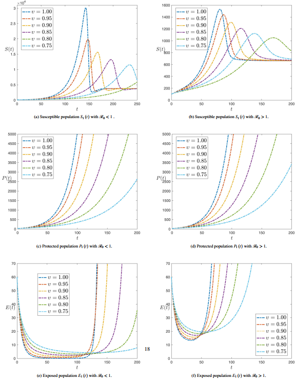
Figure 1 shows the numerical simulation of plant compartments Susceptible ${\textstyle S_{1}\left(t\right)}$, Protected ${\textstyle P_{1}\left(t\right)}$ and Latent ${\textstyle E_{1}\left(t\right)}$ with time history for various values of fractional order at ${\textstyle \mathrm {\mathcal {R}} _{0}<1}$ and ${\textstyle \mathrm {\mathcal {R}} _{0}>1}$. Figures 1(a) and 1(b) show that the maximum value of ${\textstyle S_{1}(t)}$ decreases whether ${\textstyle \mathrm {\mathcal {R}} _{0}<1}$ and ${\textstyle \mathrm {\mathcal {R}} _{0}>1}$, as the time increases and the fractional-order decreases. Figures 1(c) and 1(d) show that ${\textstyle P_{1}(t)}$ decreases as the fractional order decreases and on a big difference between the situation when ${\textstyle \mathrm {\mathcal {R}} _{0}<1}$ and ${\textstyle \mathrm {\mathcal {R}} _{0}>1}$. Figure 1(e) shows that ${\textstyle E_{1}(t)}$ decreases dramatically during the first period with increasing the fractional order until it reaches about 120 days, and then the process reverses after that. While Figure 1(f) shows that ${\textstyle E_{1}(t)}$ is decreasing, but only until 50 days before it starts increasing again.

Figure 1. Numerical simulation of plant compartments $S_{1}\left(t\right),P_{1}\left(t\right),E_{1}\left(t\right)$ for various values of fractional order with $\mathrm {\mathcal {R}} _{0}<1$ and $\mathrm {\mathcal {R}} _{0}>1$

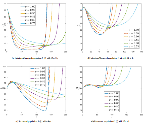
Figure 2 shows the numerical simulation of plant compartments Infected ${\textstyle I_{1}\left(t\right)}$ and Removed ${\textstyle R_{1}\left(t\right)}$ with time history for several values of fractional order at ${\textstyle \mathrm {\mathcal {R}} _{0}<1}$ and ${\textstyle \mathrm {\mathcal {R}} _{0}>1}$. Figure 2(a) shows that ${\textstyle I_{1}(t)}$ initially decreases until close to 150 days with the value of the fractional order differing, and then the process reverses after that. While Figure 2(b) shows that ${\textstyle I_{1}(t)}$ decreases until the period from 60 to 80 days, but its value does not reach zero on the vertical axis, as happened with Figure 2(a).

Figure 2. Numerical simulation of plant compartments $I_{1}\left(t\right),R_{1}\left(t\right)$ for various values of fractional order with $\mathrm {\mathcal {R}} _{0}<1$ and $\mathrm {\mathcal {R}} _{0}>1$

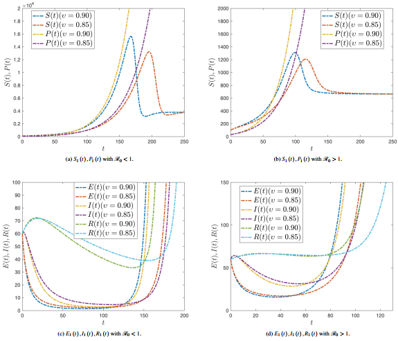
Figure 3 shows the numerical simulation of plant compartments ${\textstyle S_{1}\left(t\right)}$, ${\textstyle P_{1}\left(t\right)}$, ${\textstyle E_{1}\left(t\right)}$, ${\textstyle I_{1}\left(t\right)}$ and ${\textstyle R_{1}\left(t\right)}$ with time history for various values of fractional order at ${\textstyle \mathrm {\mathcal {R}} _{0}<1}$ and ${\textstyle \mathrm {\mathcal {R}} _{0}>1}$.

Figure 3. Numerical simulation of plant compartments $S_{1}\left(t\right),P_{1}\left(t\right),E_{1}\left(t\right),I_{1}\left(t\right),R_{1}\left(t\right)$ with $\mathrm {\mathcal {R}} _{0}<1$ and $\mathrm {\mathcal {R}} _{0}>1$

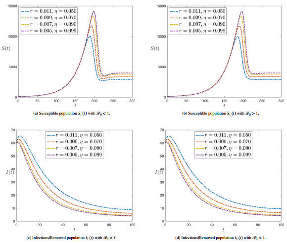
Figure 4 shows the dynamic compartments of Susceptible and Infected with various roguing and replanting values at ${\textstyle \upsilon =0.85}$. Figures 4(a) and 4(b) show that the maximum value of ${\textstyle S_{1}(t)}$ increases as the rate of replanting decreases and the rate of roguing increases. Figures 4(c) and 4(d) show that infectious can be increased as the rate of replanting decreases and the rate of roguing increases.

Figure 4. Dynamic compartments of Susceptible and Infected with various roguing and replanting values at $\upsilon =0.85$

Figures 5 and 6 illustrate the effect of different parameters on plant compartments of americanthe SPEIR model at ${\textstyle \upsilon =0.85}$.

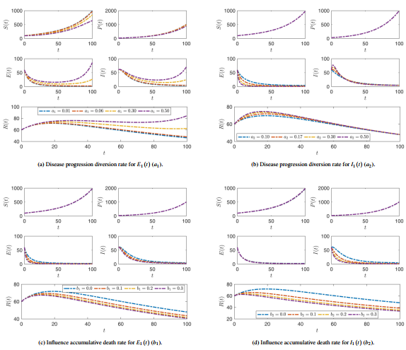
Figure 5. The effect of alteration the values of parameters $a_{1}$, $a_{2}$, $b_{1}$ and $b_{2}$ on all compartment stages where the fractional operator $\upsilon =0.85$

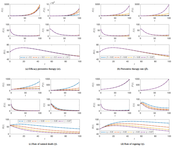
Figure 6. The effect of alteration the values of parameters $\alpha$, $\beta$, $\gamma$ and $\eta$ on all compartment stages where the fractional operator $\upsilon =0.85$

7. Conclusion

In this study, we considered and analyzed the SPEIR model displayed the dynamics of plant diseases with the Atangana-Baleanu fractional derivative in Caputo sense. Both the NEE and EE points were analyzed in terms of model equilibria and stability analysis (local-global). We also demonstrated the generic form of ${\textstyle \mathrm {\mathcal {R}} _{0}}$ and the effects of the controls proposed on it. The Adams-Bashforth-Moulton approach was used to study and solve numerical simulations of the suggested model. The value of the fractional order ${\textstyle \upsilon }$ as well as the parameters of the SPEIR model affect the numerical results that are obtained. Because of this, solutions generated by the fractional order model typically converge extremely quickly to real issues.

Conflict of Interest: The author declare that there is no Conflict of Interest.

Acknowledgments

This research project was funded by the Deanship of Scientific Research, Princess Nourah bint Abdulrahman University, through the Program of Research Project Funding After Publication, grant No (43- PRFA-P-19).

References

[1] Vanderplank J.E. Plant disease: epidemics and control. New York, Academic Press, 1963.

[2] Verhoeff K. Latent infection by fungi. Annu Rev Phytopathol, 12:99-107, 1974.

[3] Agrios G.N. Lant pathology. Academic Press, San Diego, 1988.

[4] Zhang T., Meng X., Song Y., Li Z. Dynamical analysis of delayed plant disease models with continuous or impulsive cultural control strategies. Abstract and Applied Analysis, 2012(SI12):1-25, 2012.

[5] Sisterson M.S., Stenger D.C. Roguing with replacement in perennial crops: conditions for successful disease management. Phytopathology, 103:117-28, 2013.

[6] Yang W., Wang D., Yang L. A stable numerical method for space fractional LandauLifshitz equations. Applied Mathematics Letters, 61:149-155, 2016.

[7] Kuang Y., Hu G. An adaptive FEM with ITP approach for steady Schrödinger equation. International Journal of Computer Mathematics, 95:187-201, 2018.

[8] Luo Y., Gao S., Xie D., Dai Y. A discrete plant disease model with roguing and replanting. Advances in Difference Equations, 1:1-18, 2015.

[9] Chan M.S., Jeger M.J. An analytical model of plant virus disease dynamics with roguing and replanting. Journal of Applied Ecology, 31:413-427, 1994.

[10] Blas N., David G. Dynamical roguing model for controlling the spread of tungro virus via Nephotettix Virescens in a rice field. Journal of Physics: Conference Series, 893, 012018, 2017.

[11] Anggriani N., Yusuf M., Supriatna A.K. The effect of insecticide on the vector of rice tungro disease: insight from a mathematical model. International Information Institute (Tokyo), 20:6197-206, 2017.

[12] Anggriani N., Istifadah N., Hanifah M., Supriatna A.K. A mathematical model of protectant and curative fungicide application and its stability analysis. IOP Conference Series: Earth and Environmental Science, 31, 012014, 2016.

[13] Anggriani N., et al. Optimal control of plant disease model with roguing, replanting, curative, and preventive treatment. In Journal of Physics: Conference Series, 1657, 012050, 2020.

[14] Anggriani N., et al. Dynamical analysis of plant disease model with roguing, replanting and preventive treatment. In Proceedings of 4th International Conferenve on Research, Implementation, and Education of Mathematics and Science, Yogyakarta, 14–16 May 2017.

[15] Odibat Z., Kumar S. A robust computational algorithm of homotopy asymptotic method for solving systems of fractional differential equations. Journal of Computational and Nonlinear Dynamics, 14, 081004, 2019.

[16] Momani S., Abu Arqub O., Maayah B. Piecewise optimal fractional reproducing kernel solution and convergence analysis for the Atangana–Baleanu–Caputo model of the Lienard’s equation. Fractals, 28, 2040007, 2020.

[17] Akgul A., Cordero A., Torregrosa J.R. Solutions of fractional gas dynamics equation by a new technique. Mathematical Methods in the Applied Sciences, 43:1349-1358, 2020.

[18] Singh J., Swroop R., Kumar D. A computational approach for fractional convection-diffusion equation via integral transforms. Ain Shams Engineering Journal, 9:1019-1028, 2018.

[19] Caputo M., Fabrizio M. A new definition of fractional derivative without singular kernel. Progress in Fractional Differentiation and Applications, 1:73-85, 2015.

[20] Abu Arqub O., Singh J., Maayah B., Alhodaly M. Reproducing kernel approach for numerical solutions of fuzzy fractional initial value problems under the Mittag–Leffler kernel differential operator. Mathematical Methods in the Applied Sciences, 46(7):7965-7986, 2023.

[21] Baleanu D., Mousalou A., Rezapour S. On the existence of solutions for some infinite coefficient-symmetric Caputo-Fabrizio fractional integro-differential equations. Boundary Value Problems, 1:1-9, 2017.

[22] Teodoro G., et al. A review of definitions of fractional derivatives and other operators. Journal of Computational Physics, 388:195-208, 2019.

[23] Atangana A., Baleanu D. New fractional derivatives with nonlocal and non-singular kernel: theory and application to heat transfer model. Thermal Science, 20:763-769, 2016.

[24] Maayah B., Abu Arqub O., Alnabulsi S., Alsulami H. Numerical solutions and geometric attractors of a fractional model of the cancer-immune based on the Atangana-Baleanu-Caputo derivative and the reproducing kernel scheme. Chinese Journal of Physics, 80:463-483, 2022.

[25] Abu Arqub O., Singh J., Alhodaly M. Adaptation of kernel functions‐based approach with Atangana–Baleanu–Caputo distributed order derivative for solutions of fuzzy fractional Volterra and Fredholm integrodifferential equations. Mathematical Methods in the Applied Sciences, 46:7807-7834, 2023.

[26] Djennadi S., Shawagfeh N., Abu Arqub O. Well-posedness of the inverse problem of time fractional heat equation in the sense of the Atangana-Baleanu fractional approach. Alexandria Engineering Journal, 59:2261-2268, 2020.

[27] Akgül A. A novel method for a fractional derivative with nonlocal and non-singular kernel. Chaos, Solitons Fractals, 114:478-482, 2018.

[28] Jajarmi A., Ghanbari B., Baleanu D. A new and efficient numerical method for the fractional modelling and optimal control of diabetes and tuberculosis co-existence. Chaos: An Interdisciplinary Journal of Nonlinear Science 29, 093111, 2019.

[29] Yildiz T.A., et al. New aspects of time fractional optimal control problems within operators with nonsingular kernel. Discrete & Continuous Dynamical Systems-S, 13:407-28, 2020.

[30] Sardar T., et al. A generic model for a single strain mosquito-transmitted disease with memory on the host and the vector. Mathematical Biosciences, 263:18-36, 2015.

[31] Podlubny I. Fractional differential equations. Academic Press, New York (1999).

[32] Gorenflo R., Mainardi F. Fractional calculus: Int and differential equations of fractional order. In A. Carpinteri, F. Mainardi (Eds.), Fractals and Fractional Calculus, New York, 1997.

[33] Driessche P., Watmough J. Reproduction numbers and sub-threshold endemic equilibria for compartmental models of disease transmission. Mathematical Biosciences, 180:29-48, 2002.

[34] Castillo-Chavez C., Feng Z., Huang W. On the computation of R0 and its role in global stability. IMA Volumes in Mathematics and Its Applications, 125:229-250, 2002.

[35] Diekmann O., Heesterbeek J.A.P. Mathematical epidemiology of infectious diseases: Model building, analysis and interpretation. John Wiley & Sons, Vol. 5, pp. 320, 2000.

[36] Nise N.S. Control systems engineering. John Wiley & Sons, 8th edition, pp. 800, 2020.

[37] Verhulst F. Nonlinear differential equations and dynamical systems. Springer, Heidelberg, pp. 306, 1996.

[38] Wiggins S. Introduction to applied nonlinear dynamical systems and chaos. Part of the book series: Texts in Applied Mathematics (TAM, volume 2), 2nd Edition, Springer-Verlag, Heidelberg, pp. 882, 2003.

[39] Kumar D., Singh J., Baleanu D. Analysis of regularized long-wave equation associated with a new fractional operator with Mittag-Leffler type kernel. Physica A, 492:155-167, 2018.

[40] Diethelm K., Freed A.D. The FracPECE subroutine for the numerical solution of differential equations of fractional order. Forschung und wissenschaftliches Rechnen, 57-71, 1999.

[41] Garrappa Z.R. On linear stability of predictor-corrector algorithms for fractional differential equations. International Journal of Computer Mathematics, 87:2281-2290, 2010.

[42] Butcher J. Numerical methods for ordinary differential equations in the 20th century. Journal of Computational and Applied Mathematics, 125:1-29, 2000.