Multi-index cutting parameters optimization for surface quality and cutting energy consumption of boring

Abstract

Saving energy is one of the ways to achieve sustainable development. As an important equipment for manufacturing, machine tool has the characteristics of high energy consumption and high emission. In order to cope with reducing energy consumption and carbon emissions without reducing processing quality, the search for optimal cutting parameters requires balancing the contradiction between machining quality and cutting energy consumption, so that cutting parameters can both reduce energy consumption and ensure the quality of processing. It plays an important role in achieving energy saving and emission reduction. In this paper, the processing quality (residual stress, surface roughness) and cutting energy consumption are selected as the optimized multiple indicators, and the selected optimization indicators are analyzed. Weighted grey correlation analysis is used to obtain the multi-index gray correlation degree value, and the multi-index weight coefficient is determined. Based on weighted grey correlation analysis and multi-index orthogonal optimization method, the cutting parameters of the boring process are optimized, and the optimal parameter combination is that cutting depth of 0.05 mm, cutting speed of 120 m/min, and feed rate of 80 mm/min.

Keywords: Boring, cutting energy consumption, surface quality, grey relational analysis, multi-index orthogonal optimization

1. Introduction

With the increase in energy demand, the price of energy has risen sharply, and the production cost of enterprises is increased. Moreover, the increasing awareness of environmental protection demands the restriction of carbon emissions. Therefore, manufacturers are eager to reduce energy consumption and make full use of resources to reduce the carbon dioxide emissions of the manufacturing process. Obviously, energy conservation and emission reduction have become the top priority of the manufacturing industry. In the machining process, the choice of cutting parameters directly affects the surface quality, energy consumption, and environmental emissions of the parts. According to research, selecting the best cutting parameters and optimizing tool trajectory can achieve up to 6-40% energy-saving effect [1]. In addition, energy consumption during processing is also a major part of the environmental burden. Therefore, it is particularly important to optimize cutting parameters and reduce energy consumption of machine tools.

Xie et al. [2] systematically studied the energy consumption characteristics of the whole process of machine tool operation, and constructed the energy consumption cutting parameter model of the whole process of workpiece processing. On this basis, they proposed an energy saving decision method about cutting model for high energy consumption and low emission. Liu et al. [3] proposed a method for energy consumption optimization of CNC machine tools based on cutting parameters. By determining the optimization variables and objective functions of cutting parameters, adding energy consumption constraints for CNC machine tools, and solving the energy consumption optimization function of CNC machine tools based on cutting parameters. Deng et al. [4] established a multi-objective optimization model with milling time and energy consumption as the optimization goals, combined with the actual constraints in the milling process, and took the spindle speed, feed rate, and milling width as the optimization variables, using particles Group algorithm (PSO) finds the optimal solution for the target model. Through actual milling experiments, the validity of the built model is verified, and the optimization results are analyzed. Chandgude et al. [5] used an overall hard TiAlN coating end mill to machine AISI D2 hardened steel to obtain experimental data, and used principal component analysis to optimize cutting parameters. Jiang et al. [6] proposed a cutting parameter optimization model that considers the minimum cutting fluid consumption and the minimum machining cost. Machining cost and cutting fluid consumption were regarded as two goals in the optimization model. A hybrid genetic algorithm was used to solve multi-objective problems and the best cutting parameters was obtained. Balaji et al. [7] used orthogonal methods and analysis of variance to perform drilling experiments. The surface roughness and amplitude were used as targets to evaluate the tool life and cutting parameter significance, and to obtain the optimal cutting parameter level. Rajesh et al. [8] used high-speed steel tools to carry out turning experiments on Al6061 workpiece materials under different cutting parameter values. With the aim of cutting temperature and surface roughness, a regression model related to cutting temperature and surface roughness was established and then passed on. The algorithm to get the best value of the cutting parameters. Chávez-García et al. [9] proposed a novel simulation-based multi-objective optimization (SimMOpt) solution program, which optimizes machining time, processing cost, and product quality to obtain the best cutting parameter conditions. From the above optimization study of cutting parameters, it is shown that the most commonly used optimization targets in machining are traditional indicators such as processing time, processing cost, product quality, and tool life. The optimization methods for such machining processes do not involve environmental issues. Far from meeting the requirements of modern processing.

Economic sustainability has always been the main focus of the optimization of processing operations, and environmental sustainability is rarely taken seriously. Obviously, reducing the machining energy consumption of machine tools can significantly improve the environmental performance of manufacturing process. In actual production, the selection of suitable cutting parameters is of great significance for promoting machining efficiency, reducing energy consumption and ensuring machining quality. Generally, the selection of cutting parameters usually depends on experience or the use of the cutting volume manual. It is feasible to use this method, but it is difficult to get the optimal cutting parameters, and the processing quality cannot be guaranteed, and even more energy will be consumed. In recent years, research has begun to consider energy consumption to choose the best cutting parameters. Mativenga et al. [10] through the turning experiment to optimize the minimum energy footprint, using the direct search method to select the best cutting parameters. Kuram et al. [11] studied the effects of cutting fluid type on the process response (specific energy consumption, tool life and surface roughness) through milling experiments. The D-optimal method was used for experimental design and the target was specific energy consumption. Tool life and surface roughness were used as invisible constraints to optimize the cutting parameters. Based on the optimization results, various conclusions about the effects of cutting parameters and cutting fluid types on the milling performance criteria were obtained. Bhushan et al. [12] aimed at the lowest processing energy consumption and the best tool life. The response surface method was used to optimize the turning parameters. Campatelli et al. [13] optimized the energy consumption as the minimum, and also adopted response surface methodology to optimize the cutting parameters and minimize the energy consumption during the milling process on the machining center. Velchev et al. [14] improved the traditional specific energy consumption model and combined the turning experiment to design the optimal cutting parameters by applying the minimum energy standard. Kant et al. [15] proposed a framework to solve the multi-objective optimization problem. Using the minimum total energy consumption and the minimum total tardiness time as targets, a greedy stochastic adaptive search heuristic algorithm was used to obtain the approximate Pareto front solution. Then use the analytic hierarchy process to determine the optimal solution. Liu et al. [16] proposed a multi-objective optimization model for high-efficiency low-carbon manufacturing cutting parameters with cutting speed and feed rate as the optimal variables, carbon emissions and processing time as the optimization objectives, and non-dominated sorting genetic algorithm for optimal turning. The cutting parameters of the process Zhang et al. [17] optimized the minimum carbon emissions and the minimum processing time for multiple objectives. An improved multi-objective gravity search algorithm combining crossover and mutation operators was designed to find the optimal solution. Based on milling experiments, Zhang et al. [18] established an optimization model with the target of minimum specific energy consumption and minimum processing time, and introduced the quantum weight of subjective and objective weights to solve the optimal cutting parameters of the milling process through a quantum genetic algorithm. However, many of these studies only focus on the minimum energy consumption of cutting parameters. It is important to achieve the minimum processing energy consumption for the development of green sustainable manufacturing, but paying attention to the processing quality to obtain an excellent processing surface is also one of the optimization goals that must be taken seriously in processing. It is obviously more reasonable to optimize the cutting parameters based on the machining quality and cutting energy consumption. In addition, most of the optimization models established by most researchers use the same weights or select a weight to subjectively emphasize or weaken the target, so as to optimize the cutting parameters for single-objective or multi-objective optimization. This lacks a reasonable quantitative basis. Therefore, it is necessary to objectively calculate the weight factors, and it is necessary to formulate a reasonable standard so that appropriate values can be assigned to different optimization objectives during the optimization process.

2. Experimental design

2.1 Experimental material and processing platform

The experimental material is grey cast iron HT200, the sample size is 85mmà64mmà20mm, the chemical composition and mechanical properties are shown in Tables 1 and 2.

Table 1. Chemical composition of gray cast iron HT200

C (%)	S (%)	Mn (%)	P (%)	Si (%)
3.0～3.6	≤0.12	0.6～1.0	≤0.15	1.4～2.2

Table 2. Mechanical properties of gray cast iron HT200

Shear modulus Gpa	Flexural strength Gpa	Density kg/m3	Poisson's ratio	Elastic Modulus Gpa
56.6	0.2	7200	0.31	148

The machine tool is MCV-810 machining center (produced by Taiwan Seiki Corporation), the maximum spindle speed is 8000 r / min, the maximum power of the machine tool is 20 kVA, and the system is the FANAC CNC system.

The cutting force data acquisition system is made up of a cutting force measurement system composed of Kistler9257B type piezoelectric sensor, Kistler5080 charge amplifier, Kistler5697 data collector, computer and Dyno Ware2825D software. The WT330 series power meter produced by Henghe company (YOKOGAWA) is used to measure the power of machine tools during processing.

For boring machining, NBJ16 is chosen as the center of fine tuning and boring cutter machining center. The universal blade of the boring bar is KYOCERA blade, and the TBGT060102L blade is chosen. The test platform is shown in Figure 1, and the cutting fluid is used in the machining process.

Figure 1. Experimental processing platform schematic

2.2 The measuring instrument of surface quality

The instrument used for surface quality observation is shown in Table 3. The surface roughness measurement uses the contour arithmetic mean deviation Ra as the surface roughness evaluation parameter. The measurement parameters are selected as follows: the sampling length is 0.8 mm, the evaluation length is 4 mm, and the measurement length is 5.6 mm. The residual stresses in the surface layer of the gray cast iron after boring were measured by X ray diffraction using the protoiXRD residual stress tester.

Table 3. Surface quality observation instrument

Instrument name	Model and place of origin
Roughness Tester	Mahr XR20, Mahr, Germany
Scanning electron microscope	TM3030, Hitachi Company, Japan
Three-dimensional digital microscope	KH-1300, HIROX Corporation, Japan
Residual stress measuring	protoiXRD, Proto company, Canada

2.3 Experimental Procedures and Parameters

In this test, Fine boring was carried out first, and then a small sample was obtained by wire cutting. Before the observation, the workpiece was cleaned with an acetone solution in an ultrasonic vibration cleaner for 20 minutes, and finally dried and then surface quality indicators after fine boring were examined. In order to avoid surface scratches, the residual stress was measured before measuring the surface roughness, and then the scanning electron microscope and three-dimensional digital microscope were observed, and finally the surface roughness was measured. To reduce the experimental error, each set of parameters was tested 3 times and averaged. Single factor experiments and $L_{16}$ ($4^{5}$) orthogonal experiments were designed as shown in Tables 4 and 5.

Table 4. Boring single factor experimental parameters

Cutting elements	Value
$a_{p}$ (mm)	0.05, 0.15, 0.25, 0.30, 0.35
$v_{c}$ (m/min)	90, 120, 150, 180, 210
$v_{f}$ (m/min)	30, 50, 80, 110,130
$a_{p}$ (mm)	0.05, 0.15, 0.25, 0.30, 0.35

Table 5. Orthogonal experimental factor level table

Factors Level	$a_{p}$ (mm)	$v_{c}$ (m/min)	$v_{f}$ (m/min)
Level 1	0.05	120	30
Level 2	0.15	150	50
Level 3	0.25	180	80
Level 4	0.35	210	110

3. Cutting parameter optimization multiple indicators selected

Energy saving is the way of sustainable development. As an important equipment in manufacturing industry, machine tools have the characteristics of high energy consumption and high emission. In order to reduce the energy consumption and improve the energy efficiency without reducing the quality of processing, it is necessary to weigh the cutting energy and processing quality to find the best cutting parameters. For contradiction, cutting parameters can not only reduce energy consumption, but also ensure machining quality. It plays an important role in energy saving and emission reduction. The aim of this paper is to balance the contradiction between the cutting energy and the processing quality in the precision boring process. The grey correlation theory and the multi-index orthogonal optimization method are used to find the optimal cutting parameters. The target is called the target in the orthogonal optimization (the target city will be the index below). The framework, index and cutting parameters of the optimization problem are outlined in Fig 2. The multiple parameters of the cutting process are cutting energy consumption and machining quality, in which the surface roughness, surface micromorphology, surface residual stress and surface microhardness are measured, and the cutting energy consumption and processing quality will be analyzed from the following. And choose the index. The three important cutting parameters are back feed, cutting speed and feed speed.

Fig 2. Frame structure between optimization problems, indexes and cutting parameters

3.1 Analysis of cutting energy consumption

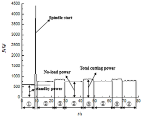
Fig 3 is the power profile of the boring process obtained during the cutting process of the machining center MCV-810. The time period ① is the standby machine running state of the machine tool, the time ② is the state of the machine tool no-load operation, and the time ③ is the cutting and working state of the machine tool. The cutting energy can be calculated by the power meter to detect the required cutting power and the product of the cutting time. As shown in formula (1), the Ec is the cutting energy (unit: J), the Pc is the cutting power (unit: W), and the Tc is the time used for boring a single hole (unit: s).

$Grade=\sum _{i=I}^{m}{\omega }_{i}GRC_{i}$

$E_{c}=P_{c}\times T_{c}$ （1）

Fig 3. The power profile of the MCV-810 boring process

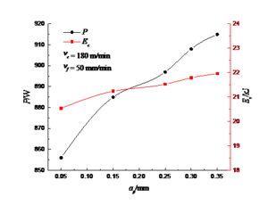
Figs 4 to 6 are the effects of different cutting parameters on cutting power and energy consumption. As can be seen from Fig 4 and Fig 5, the cutting power and energy consumption increases with the increase of the back knife and cutting speed. This is because the higher the cutting parameters, the higher the cutting parameters, the higher the load, the greater the cutting power and the energy consumption in the case of fixing the other two cutting elements; as shown in Fig 6, with the feed speed. With the increase of the cutting power, the cutting energy is reduced, and the higher the feed speed is, the higher the feed speed is, the higher the machine tool load, so the cutting power will increase, but the machining time is shortened, and the cutting energy consumption will be reduced. Power cannot reflect the energy consumption during the actual cutting process, although power cannot reflect the energy consumption in the actual cutting process. The actual cutting energy needs to be determined by the power and time. Therefore, considering the traditional and sustainable factors, it is a more reasonable multi-index optimization method to consider cutting energy consumption rather than power.

Fig 4. The effect of the back cutting depth on the cutting power and energy consumption

Fig 5. The effect of the cutting speed on cutting power and energy consumption

Fig 6. The effect of the feed rate on cutting power and energy consumption

3.2.1 Surface roughness analysis

During the cutting process, the surface roughness of the workpiece has been affected by many factors, such as residual area, vibration, built-up lump, scale thorn, workpiece material and so on. The specific cutting conditions are also reflected in the cutting force, and the machined surface roughness can be analyzed according to the cutting force. Therefore, the surface roughness of the gray cast iron boring is studied and analyzed in this paper.

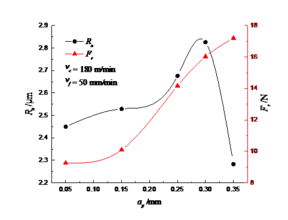
Fig. 7 is the influence of the back cutting depth on the surface roughness and cutting force. As can be seen from the diagram, the cutting force increases with the increase of the back cutting depth, while the surface roughness increases with the back cutting depth increase when the back cutting depth is less than 0.30 mm, and the surface roughness decreases when the a_p is equal to 0.35 mm. When the back cutting depth is increased, the system is easy to be in unstable state and easily flutter because of the longer hanging of the boring bar and the friction between the back and the inner holes of the tool. At the same time, the volume of the material is increased and the cutting force of the material increases, which leads to the increase of the surface roughness. When the amount of the back knife is equal to 0.35 mm, the back cutting depth is larger, because the heat of the friction between the tool and the workpiece produces enough heat to produce the softening effect of the metal in the cutting area, which reduces the tool wear speed and causes the surface roughness to decrease suddenly. However, the back cutting depth is too large, no matter the cutting force or the cutting area, and the surface roughness decreases.

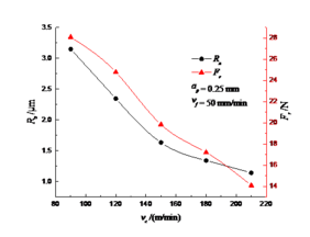
Fig. 8 is the effect of cutting speed on surface roughness and cutting resultant force. From the graph, the resultant force and surface roughness decrease with the increase of cutting speed. With the increase of cutting speed, the scraps and spines are reduced and the cutting forces are reduced. At the same time, the frequency of the system is far away from the inherent frequency of the machine system because of the increase of the cutting speed, thus reducing the vibration of the system and reducing the surface roughness.

Fig. 9 is the influence of feed speed on surface roughness and cutting resultant force. From the graph, the resultant force and surface roughness increase with the increase of feed speed. With the increase of feed speed, on the one hand, the effect of the cutting tool and the machining surface is enhanced, the greater the surface area of the surface, the increase of the metal deformation resistance and the increase of the cutting force, so the roughness of the surface increases rapidly. On the other hand, the vibration of the machining system is aggravated, and the surface roughness increases.

Fig 7. The effect of the back cutting depth on the surface roughness

Fig 8. The effect of the cutting speed on the surface roughness

Fig 9 The effect of the feed rate on the surface roughness

3. 2.2 Analysis of surface micromorphology

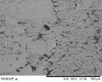
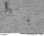
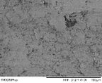
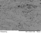
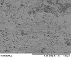
Fig. 10 to Fig. 12 are observation results of the surface morphology of gray cast iron boring under different cutting parameters. The results are obtained by observing the KH-1300 three-dimensional digital microscope and scanning electron microscope TM3030. The magnification of the KH-1300 three-dimensional digital microscope is: 70 times, scanning electron microscope TM3030 magnification of 1000 times. The surface characteristics of Fig. 10 to Fig. 12 can be observed by means of the KH-1300 three-dimensional digital microscope. In particular, the distribution of the surface texture is very different. The surface roughness Ra is 2.450, 2.826, and 3.151μm in order of arrangement in the Fig. 10 to Fig. 12. When the surface roughness is small, the surface texture is finely distributed. On the other hand, the distribution interval is large. According to the results of SEM observation, the gray cast iron materials mainly consist of brittle fractures. Graphite is detached from the surface of cast iron to form pits during cutting, and the sharp edges of graphite lamella structure of flake graphite are easy to form irregular cracks and fractures. Affects the integrity of the machined surface.

Fig.10 compares the surface topography under different back-feeding amount. It can be seen from Fig.10 (a₁) and (a₂) that the width of the surface texture slightly increases with the increase of the back knife, and the surface roughness increases. Slightly increased. Fig.8 shows the comparison of surface topography at different cutting speeds. It can be seen from Fig.11 (a₁) and (a₂) that as the cutting speed increases, the surface texture is denser and more uniform, the surface roughness is reduced, and the surface quality is improved. Comparing the scanning electron microscopy image of Fig.11, Fig.11(b₁) shows that the lower cutting speed is more pronounced with pits, while Fig.11(b₂) is smoother and flatter. Fig.12 shows the comparison of the surface topography at different feed rates. In the case of a small feed, the texture of the workpiece surface is relatively narrow. It can be seen from Fig.12(b₁) that the machined surface is relatively smooth and smooth. Comparing Fig.12 (a₁) and (a₂), as the feed rate increases, the surface texture of the workpiece changes from shallow to deep, from narrow to wide, the surface roughness increases, and pits on the surface of the material also increase, brittle fracture characteristics are obvious. The surface quality has deteriorated significantly.

(a1) ap=0.05mm	(b1) ap = 0.05mm
(a2) ap = 0.30mm	(b2) ap = 0.30mm

Fig 10. Comparison of the surface topographies of different the back cutting depth (v_c=180m/min, v_f=50mm/min): (a) KH-1300 three-dimensional digital microscope 70 times; (b) electron microscope TM3030 1000 times

(a1) vc = 90m/min	(b1) vc = 90m/min
(a2) vc = 210m/min	(b2) vc = 210m/min

Fig 11. Comparison of surface morphology at different cutting speeds (a_p=0.25mm, v_f=50mm/min): (a) KH-1300 three-dimensional digital microscope 70 times; (b) electron microscope TM3030 1000 times

(a1) vf = 30mm/min	(b1) vf = 30mm/min
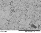
(a2) vf = 130mm/min	(b2)vf= 130mm/min

Fig 12. Comparison of surface topography at different feed rates (a_p=0.25mm, v_c=180m/min): (a) KH-1300 three-dimensional digital microscope 70 times; (b) electron microscope TM3030 1000 times

3.2.3 Surface Residual Stress Analysis

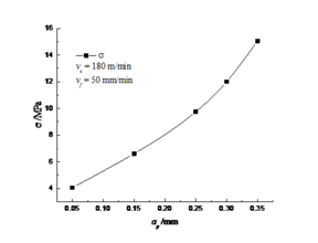
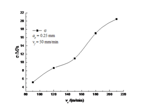
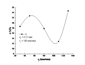
Figs 13 to 15 show the influence of the back-side knife, cutting speed, and feed rate on the residual stress of the machined surface. It can be seen from the Fig that the residual stress is tensile stress. Residual stress is the result of the combined effect of cutting force and cutting heat. In the processed surface cutting force, compressive stress is generated, and cutting heat generates tensile stress. As the cutting speed of the boring and finishing is higher, the generated cutting heat is more, so the residual is present. Pull stress. The residual stress on the surface of the grey cast iron is increased with the increase in the amount of backing and the cutting speed. With the increase of the back knife, the residual stress of the surface layer increases. This is because when the amount of the back knife increases, the friction between the blade and the material increases, the cutting temperature increases, and the thermal stress generated on the surface of the material increases. Larger results in increased residual stress; similarly, when the cutting speed increases, the cutting temperature increases, the heat increases rapidly, the heat transferred to the surface layer increases, and the residual stress of the surface layer increases, while the feed rate increases, the surface layer increases. The residual stress shows a curve change. When the feed-rate is low, the residual stress shows a growing trend. When the feed-rate reaches a certain stage, the cutting heat is too late to transmit to the workpiece. Therefore, the residual stress is reduced at this time, and then the feed-rate is increased. The influence of the deformation zone becomes greater, and at the same time the cutting temperature is further increased, so that the effect of thermal stress continues to increase and the residual stress increases.

Fig 13. Effect of the back cutting depth on residual stress of processed surface layer

Fig 14. Effect of the cutting speed on the residual stress of the processed surface layer

Fig 15. Effect of the feed rate on the residual stress of the processed surface layer

3.3 Multiple indicator optimization selected

The influence of the cutting parameters on the surface quality of the boring, including surface roughness, surface micro-morphology, and surface residual stress, was analyzed above, and the surface roughness and surface residual stress are widely used to evaluate the quality of the product, and its cutting parameters. There is a big relationship, so the multi-targets optimized for this boring process are determined as surface roughness, surface residual stress and cutting energy consumption. According to the frame structure between the optimization problem, index and cutting parameters in Fig 2, formula (2) can be used to describe the multi-objective optimization problem, where Ra is the surface roughness, σ is the surface residual stress, and Ec is the cutting energy consumption.

${\textstyle \left\{{\begin{matrix}min{R}_{a}({a}_{p},{v}_{c},{v}_{f})\\min\sigma ({a}_{p},{v}_{c},{v}_{f})\\minEc({a}_{p},{v}_{c},{v}_{f})\end{matrix}}\right.\left\{{\begin{matrix}{a}_{pmin}\leq {a}_{p}{\leq a}_{pmax}\\{v}_{cmin}\leq {v}_{c}{\leq v}_{cmax}\\{v}_{fmin}\leq {v}_{f}{\leq v}_{fmax}\end{matrix}}\right.}$ (2)

The key to the optimization of the cutting parameters in this paper lies in weighing the contradictions between cutting energy consumption and processing quality (surface roughness and surface residual stress). The steps of cutting parameter optimization are shown in Fig 16. First, the optimization index based on the trade-off problem framework (introduced above) is determined; secondly, the orthogonal experiment is used to design the experiment and data acquisition (introduced above); then the grey correlation is combined. Calculate the weights of each index in theory to determine the comprehensive scoring formula: normalize the index values that need to be optimized, and then calculate the gray correlation coefficient of each index to determine the weight coefficient assigned to each index in the comprehensive scoring method; The index orthogonal optimization comprehensive scoring method selects the optimal cutting parameters.

Fig 16. cutting parameters optimization steps

4. Optimized calculation process

4.1 Grey relational theory calculation

Grey relational analysis is based on grey relational theory and is used to effectively solve the interrelationships of complex multiple response indicators. The grey relational theory was used to determine the relationship between the multi-index orthogonal optimization comprehensive score Grade, and the steps are as follows [19].

1. Normalize the experimental results of the indicators (surface roughness and cutting energy consumption) that need to be optimized to avoid the influence of different units on the calculation. If the index value is "bigger is better", then the normalization adopts formula (3); if the index value is "smaller, the better", then formula (4) is used.

${\textstyle {Z}_{ij}={\frac {{y}_{ij}-min({y}_{ij},i=1,2,\cdots ,n)}{max({y}_{ij},i=1,2,\cdots n)-min({y}_{ij},i=1,2,\cdots n)}}}$

(3)

${\textstyle {Z}_{ij}={\frac {max({y}_{ij},i=1,2,\cdots n)-{y}_{ij}}{max({y}_{ij},i=1,2,\cdots n)-min({y}_{ij},i=1,2,\cdots n)}}}$

(4)

Where i = 1, 2, ..., n and j = 1, 2, ...; m. n is the number of experiment groups and m is the number of optimization indicators. Because the index values (surface roughness and cutting energy consumption) optimized in this paper are "smaller is better", the normalized calculation uses equation (4). The results are shown in Table 6.

2. Calculate the normalized Grey Relational Coefficient (GRC).

${\textstyle \gamma (Z_{O},Z_{ij})={\frac {\Delta min+\xi \Delta max}{{\Delta }_{oj}(k)+\xi \Delta max}}}$

(5)

Where Zo(k)is the reference sequence (Zo(k) = 1, k = 1, 2, …, m), and △oj(k) is the deviation sequence of the reference sequence Zo(k) and the comparison sequence Zij(k). That is, △oj(k)= || Zo(k) - Zij(k)||. △max = max△oj(k) is the maximum value of △oj(k), and △min = min△oj(k) is the minimum value of△oj(k). ξ is the resolution factor. The value range is 0 ≤ ξ ≤1, and ξ is usually 0.5 [20]. The results are shown in Table 6.

Table 6. Normalized value and grey correlation coefficient

	Normalized value				Gray correlation coefficient
Experiment number		Normalization of σ	Normalization of Ra	Normalization of Ec	GRCσ	GRCRa	GRCEc
1	1.00		0.69	0.20	0.00	0.30	0.79
2	0.70		0.79	0.62	0.29	0.20	0.37
3	0.56		0.90	0.86	0.43	0.09	0.13
4	0.20		1.00	0.86	0.79	0.00	0.03
5	0.64		0.46	0.63	0.35	0.53	0.36
6	0.76		0.70	0.10	0.23	0.29	0.89
7	0.39		0.59	0.97	0.60	0.40	0.02
8	0.52		0.90	0.79	0.47	0.09	0.20
9	0.64		0.23	0.85	0.35	0.76	0.14
10	0.29		0.33	0.97	0.70	0.66	0.02
11	0.57		0.71	0.03	0.42	0.28	0.96
12	0.33		0.76	0.51	0.66	0.23	0.48
13	0.00		0.00	1.00	1.00	1.00	0.00
14	0.38		0.32	0.84	0.61	0.67	0.15
15	0.29		0.48	0.54	0.70	0.51	0.45
16	0.31		0.73	0.00	0.68	0.26	1.00

3. The weight coefficient ω is calculated. For a multi-index optimization problem, the importance of each indicator is different. Under the condition that the importance of each indicator is not equal, there is a great change in the degree of gray correlation, which means that the weight coefficient is very good for the optimal outcome trade-off. important. In general, the same weights are used to calculate the grey correlation of multiple response indicators, or the degree of importance of the optimization indicators is determined by experience, but such processing lacks a reasonable quantitative basis. Therefore, in order to objectively calculate the weight coefficient, it is necessary to formulate a reasonable standard so that different weight coefficients can be assigned to different indicators in the optimization process. The weight coefficient ω is calculated by first normalizing the experimental results of the optimized index, then calculating the grey correlation coefficient of the optimized index, taking the gray correlation coefficient of each cutting parameter level as average, and then obtaining the grey correlation coefficient at each level. The ratio of the mean R(max-min), the ratio of the average of the difference between the mean value of the grey correlation coefficient of each optimization index and the sum of the mean difference of the gray correlation coefficient of all the optimization indexes is the weight coefficient ω, and the calculation formula is as follows. The specific calculation results are shown in Table 7.

$R_{I,j}=max\left\{K_{I,j,1},K_{I,j,2},\cdots ,K_{I,j,k}\right\}-$$min\left\{K_{I,j,1},K_{I,j,2},\cdots ,K_{I,j,k}\right\}$ （6）

${\omega }_{i}={\frac {\sum _{j=1}^{p}R_{I,j}}{\sum _{i=1}^{m}\sum _{j=1}^{p}R_{I,j}}}$ （7）

Where i = 1, 2, …, m; j = 1, 2, …, p; k= 1, 2, …, l. m is the number of optimization indicators, p is the number of orthogonal experimental factors, l is the number of orthogonal experimental levels, K is the average value of gray correlation coefficients at each level, and R is the average value of the gray correlation coefficients at each level Worse, ω is the weight coefficient of the optimization indicator.

Table 7. Average of gray correlation coefficients at each level

	σ			Ra	Ec		σ
	ap	vc	vf	ap	vc	vf	ap	vc	vf
Level 1	0.6376	0.6256	0.6593	0.7927	0.4578	0.6359	0.6734	0.6832	0.3552
Level 2	0.5577	0.5430	0.5146	0.6272	0.5497	0.5918	0.6487	0.6631	0.5449
Level 3	0.4919	0.4856	0.5202	0.5355	0.6304	0.6255	0.6441	0.6515	0.7612
Level 4	0.4043	0.4372	0.3974	0.4760	0.7935	0.5782	0.6562	0.6246	0.9610
Range	0.2334	0.1884	0.2619	0.3168	0.3357	0.0576	0.0293	0.0586	0.6058
∑range		0.6837		0.7101			0.6936
Weight		32.76%		34.02%			33.23%

4. Determine the relation of multiple indicators orthogonal optimization comprehensive score Grade by grey relational theory.

$Grade=\sum _{i=I}^{m}{\omega }_{i}GRC_{i}$

(8)

According to the above calculation, the weight coefficient of the surface roughness Ra is 51.88% and the weight coefficient of the cutting energy consumption Ec is 48.12%, which is shown by the formula (9) of the multi-index orthogonal optimization comprehensive score Grade.

${\textstyle Grade=32.76\%\times GR{C}_{a}+34.02\%\times GR{C}_{Ra}+}$$33.23\%\times GR{C}_{Ec}$

(9)

4.2. Multi index optimization

The calculation is performed according to the relationship (9) of the quasi-multi-indicator orthogonal optimization score Grade, and the results are shown in Table 8. The total score reflects the situation of the two indicators. The result of the calculation of the range difference is shown in Fig 17. From the extremes of the graph and the table can be seen, the primary and secondary factors of the score: C> A> B, so A takes A₁, B takes B₁, C takes C₃. Therefore, the optimum finishing boring parameters are A₁B₁C₃, ie, the back cutting depth is 0.05 mm, the cutting speed is 120 m/min, and the feed rate is 80 mm/min.

Fig 17. Trend graph of comprehensive scores at each factor level

4.3.1. Analysis of influencing factors

After the grey relational theory calculation, according to Table 7, the main influence of each optimization index was analyzed, and the gray correlation coefficient of each index was shown in Fig 18. From Table 7 and Fig 18, it can be seen that for the residual stress gray correlation coefficient range difference Rv_f > Ra_p > Rv_c, the change of the feed rate has the largest fluctuation amplitude at the four experimental levels, followed by the back knife amount and cutting speed. , indicating that the degree of influence on residual stress is in order of feed rate, back knife, cutting speed; for the surface roughness of the gray correlation coefficient extreme difference Rv_c > Ra_p > Rv_f, the degree of influence on the surface roughness is in turn cutting Speed, back knife quantity, feed rate; for the cutting energy consumption of the gray level contact with the extreme value Rv_f > Rv_c > Ra_p, then the degree of influence on the cutting energy consumption is the feed speed, cutting speed, back knife. When the value of the three cutting elements is small, the minimum residual stress will be obtained; when the back eating amount and the feed speed are lower, the cutting speed will take the higher value, the lowest surface roughness will be obtained; The lower value of the cutting amount and cutting speed, and the higher the feed rate, will result in the lowest cutting energy consumption. However, the optimal range of these cutting parameters is not the same, meaning that it is impossible to obtain the best results for the three indicators at the same time. Therefore, using the multi-index optimization method proposed in this paper will help solve this problem.

Table 8. Test plan and results

Experimental number	A ap	B vc	C vf	σ/Mpa	Ra/μm	Ec/kJ	Grade
1	0.05	120	30	4.71	2.00	31.72	12.76
2	0.05	150	50	9.93	1.83	19.68	10.42
3	0.05	180	80	12.37	1.66	12.62	8.81
4	0.05	210	110	18.79	1.5	9.74	9.90
5	0.15	120	50	10.96	2.38	19.49	10.88
6	0.15	150	30	8.91	1.98	34.48	15.05
7	0.15	180	110	15.34	2.17	9.70	8.99
8	0.15	210	80	13.12	1.65	14.63	9.72
9	0.25	120	80	11.03	2.76	13.14	8.92
10	0.25	150	110	17.12	2.59	9.53	9.66
11	0.25	180	30	12.29	1.96	36.60	16.86
12	0.25	210	50	16.45	1.89	22.80	13.61
13	0.35	120	110	22.4	3.14	8.87	11.35
14	0.35	150	80	15.56	2.606	13.26	10.39
15	0.35	180	50	17.23	2.34	21.86	13.71
16	0.35	210	30	16.89	1.94	37.64	18.70
k1	10.47	10.98	15.84
k2	11.16	11.38	12.15
k3	12.26	12.09	9.46
k4	13.54	12.98	9.98
R	3.06	2.00	6.38

(a) The influence of the grey correlation coefficient on the residual stress index

(b) The influence of the grey correlation coefficient on the surface roughness index

(c) The influence of the grey correlation coefficient on the cutting energy consumption index

Fig.18 The influence of the grey correlation coefficient of each index

4.3.2. Comparative analysis and verification

In order to highlight the difference between the traditional optimization method and the sustainable multi-index optimization, this paper also obtains the optimal cutting parameters through the traditional optimization method. Traditional optimization refers to the optimization of parameters such as productivity, surface roughness, cutting forces, etc., regardless of environmental sustainability factors. The traditional optimization of cutting parameters in this paper assumes that the weight ratio ω between residual stress and surface roughness is 1:1. The traditional optimization result is a_p=0.05mm, v_c=120m/min, and v_f = 30 mm/min, the results of sustainable multi-index optimization in this paper are: a_p = 0.05 mm, v_c = 120 m/min, and v_f = 80 mm/min. Table 9 shows the comparison between the traditional optimization and the optimization method used in this paper. As can be seen from the table, compared with the traditional objective optimization, the cutting energy consumption has dropped from 31.72kJ to 12.12kJ, a drop of 61.79%. Due to the consideration of environmental sustainability, the shift to the direction of cutting energy consumption is optimized, although the residual stress and surface roughness increase, the increase range is relatively small. If the residual stress and surface roughness constraints are taken into account, this problem can be solved.

Table 9. Comparison of optimization results

	ap	vc	vf	σ	Ra	Ec
Do not consider the optimization of energy consumption	0.05	120	30	4.71	2.00	31.72
Consider the optimization of energy consumption	0.05	120	80	10.21	2.26	12.12

5. Conclusions

Optimizing the cutting parameters based on environmentally sustainable cutting conditions contributes to energy conservation and emission reduction in the current manufacturing industry. In this paper, the processing quality (residual stress, surface roughness) and cutting energy consumption are selected as the optimized multiple indicators, and the selected optimization indicators are analyzed. Then a combination of weighted grey correlation analysis and multiple index orthogonal optimization is proposed. The method optimizes the cutting parameters of the boring process. The main conclusions are as follows:

1. As the back cutting depth and cutting speed increase, the cutting power and energy consumption also increase. As the feed rate increases, the cutting power increases and cutting energy consumption decreases.

2. As the back cutting depth and feed rate increase, both the cutting force and the surface roughness increase, the surface micro-deformation quality deteriorates, and the residual stress of the back-feeding knife increases linearly and the feed rate remains. The stress curve changes. With the increase of cutting speed, the cutting force and surface roughness are reduced. Although the residual stress increases, the surface micro-morphology quality is improved.

3. The analysis of the impact coefficient of each index's grey correlation coefficient shows that the influence degree of residual stress is the feed rate, the back cutting depth, and the cutting speed; the degree of influence on the surface roughness is the cutting speed, backing knife amount, Feeding speed; The degree of influence on cutting energy consumption is the feed rate, cutting speed, and the back cutting depth.

According to the multi-index optimization method proposed in this paper, the optimal parameter combination is a_p= 0.05 mm, v_c= 120 m/min, and v_f = 80 mm/min.

Acknowledgements

The authors would like to gratefully acknowledge the financial support of the National Natural Science Foundation of China (Grant No. 51775113).

References

[1] Newman S, Nassehi A, Dhokia, V, et al. Energy efficient process planning for CNC machining. CIRP Journal of Manufacturing Science and Technology, 2012, 5 (2): 127-136.

[2] Xie Jun, Ma Jinghua, Luo Xiao. Research on energy-saving optimization-oriented machine tool energy consumption model and cutting parameter decision-making method［J］. Journal of Chongqing University of Technology (Natural Science), 2020, 34(8): 77-86.

[3] Liu Xia, Yao Yiping. Research on energy consumption optimization method of CNC machine tool processing based on cutting parameters[J]. Henan Science and Technology, 2020,05:73-75

[4] Deng Wei, Luo Yuyi, Luo Jingang. Milling parameter optimization based on low energy consumption[J]. Chinese Journal of Engineering Machinery. 2019,10,17(5):397-400

[5] Chandgude S B, Pawar P J, Sadaiah M. Process parameter optimization based on principal components analysis during machining of hardened steel[J]. International Journal of Industrial EngineeringComputations, 2015, 6(3): 379-390.

[6] Jiang Z, Zhou F, Zhang H, et al. Optimization of machining parameters considering minimum cutting fluid consumption[J]. Journal of Cleaner Production, 2015, 108: 183-191.

[7] Balaji M, Murthy B S N, Rao N M. Optimization of Cutting Parameters in Drilling of AISI 304 Stainless Steel Using Taguchi and ANOVA [J]. Procedia Technology, 2016, 25: 1106-1113.

[8] Rajesh N, Yohan M, Venkataramaiah P, et al. Optimization of Cutting Parameters for Minimization of Cutting Temperature and Surface Roughness in Turning of Al6061 Alloy[J]. Materials Today Proceedings, 2017, 4(8): 8624-8632.

[9] Chávez-García H, Castillo-Villar K K. Simulation-based model for the optimization of machining parameters in a metal-cutting operation[J]. Simulation Modelling Practice & Theory, 2018, 84: 204–221.

[10] Mativenga P T, Rajemi M F. Calculation of optimum cutting parameters based on minimum energy footprint[J]. Cirp Annals, 2011, 60(1): 149–152.

[11] Kuram E, Ozcelik B, Bayramoglu M, et al. Optimization of cutting fluids and cutting parameters during end milling by using D-optimal design of experiments[J]. Journal of Cleaner Production, 2013, 42(3): 159-166.

[12] Bhushan R K. Optimization of cutting parameters for minimizing power consumption and maximizing tool life during machining of Al alloy Si C particle composites[J]. Journal of Cleaner Production, 2013, 39(1): 242-254.

[13] Campatelli G, Lorenzini L, Scippa A. Optimization of process parameters using a Response Surface Method for minimizing power consumption in the milling of carbon steel[J]. Journal of Cleaner Production, 2014, 66(2): 309-316.

[14] Velchev S, Kolev I, Ivanov K, et al. Empirical models for specific energy consumption and optimization of cutting parameters for minimizing energy consumption during turning[J]. Journal of Cleaner Production, 2014, 80: 139-149.

[15] Kant G, Sangwan K S. Prediction and optimization of machining parameters for minimizing power consumption and surface roughness in machining[J]. Journal of Cleaner Production, 2014, 83: 151-164.

[16] Liu Z J, Sun D P, Lin C X, et al. Multi-objective optimization of the operating conditions in a cutting process based on low carbon emission costs[J]. Journal of Cleaner Production, 2016, 124: 266-275.

[17] Zhang Y, Liu Q, Zhou Y. Integrated optimization of cutting parameters and scheduling for reducing carbon emissions[J]. Journal of Cleaner Production, 2017, 149: 886-895.

[18] Zhang H, Deng Z, Fu Y, et al. Optimization of process parameters for minimum energy consumption based on cutting specific energy consumption[J]. Journal of Cleaner Production, 2017, 166: 1407-1414.

[19] Yan J, Li L. Multi-objective optimization of milling parameters – the trade-offs between energy, production rate and cutting quality[J]. Journal of Cleaner Production, 2013, 52(4): 462-471.

[20] Tzeng C J, Lin Y H, Yang Y K, et al. Optimization of turning operations with multiple performance characteristics using the Taguchi method and Grey relational analysis[J]. Journal of Materials Processing Technology, 2009, 209(6): 2753-2759.