Machine learning techniques to predict the compressive strength of concrete

Abstract

Conventional concrete is the most common material used in civil construction, and its behavior is highly nonlinear, mainly because of its heterogeneous characteristics. Compressive strength is one of the most critical parameters when designing concrete structures, and it is widely used by engineers. This parameter is usually determined through expensive laboratory tests, causing a loss of resources, materials, and time. However, artificial intelligence and its numerous applications are examples of new technologies that have been used successfully in scientific applications. Artificial neural networks (ANN) and support vector machine (SVM) models are generally used to resolve engineering problems. In this work, three models are designed, implemented, and tested to determine the compressive strength of concrete: random forest, SVM, and ANNs. Pre-processing data, statistical methods, and data visualization techniques are also employed to gain a better understanding of the database. Finally, the results obtained show high efficiency and are compared with other works, which also captured the compressive strength of the concrete.

Keywords

Compressive strength of concrete;

Artificial neural network;

Support vector machine;

Random forest.

1. Introduction

Conventional concrete is the most common material used in civil construction, being a mixture composed of water, cement, and different aggregates. Its resistance mainly depends on factors such as cement consumption, water-cement factor, degree of condensation, and the nature of aggregates. The compressive strength of concrete is quite considerable, but its tensile strength is much lower. Owing to this, the concrete can be classified as a fragile material, having entirely different strength properties under tensile and compression tests [1].

The compressive strength of concrete is still one of the most widely used parameters in structural engineering for the design of reinforced concrete structures. The performance of concrete, when defined empirically, can be affected by nonlinear factors by using the concrete compression test as a destructive procedure on concrete specimens. However, this activity involves time, planning, and financial cost because the commonly used compressive strength factor is obtained on the 28th day. Moreover, concrete is heterogeneous and does not follow these assumptions when it is subjected to stress and strain[2].

For fragile materials such as concrete, the most commonly used models are the Rankine and Mohr-Coulomb tests. These models are mostly applied because of their ease of use. However, in the case of concrete, they are unable to describe the strength failure accurately. This is because these models often result in high error rates in nonlinear cases [3].

Owing to the complexity of its behavior, the formulation of a complete constitutive model for concrete is difficult. Complex models have been formulated based on plasticity theory, elasticity, and computational intelligence [4–6].

Technological advancement usually allows engineering problems to be solved, with machine learning and its applications being good examples of fields explored with different expectations and realistic results. In general, artificial intelligence systems have shown their ability to solve real-life problems, particularly in nonlinear tasks [7].

Structural engineering has been a field of significant development through the implementation and testing of new computational models, predicting the different properties of concrete mixtures. In the case of behavioral models, pattern recognition is constructive, and computational intelligence methods can be used. Bio-inspired models can also be an excellent aid to the design of structures for civil engineering [8–13].

This project focuses on the use of computational intelligence to analyze and develop a prediction model for concrete compressive strength using computational methods, emphasizing accuracy and efficiency, and the potential to deal with experimental data. This study aims to contribute to a new model to determine the compressive strength of concrete, using methods such as artificial neural networks (ANNs) and support vector machines (SVMs).

2. Database

The compressive strength of concrete required a definition to establish reliable data in the literature. The chosen database was made available in the article written by Yeh [14]. The programming language used to implement these models was Python, and the Sci-kit-learn and Keras library were also used in this work. The TensorFlow was utilized for backpropagations for ANNs.

Initially, several neural networks were tested to obtain a preliminary result of the concrete compressive strength. To improve these results, other computational models and pre-processing data methods were also implemented.

2.1. Visualization and pre-processing

Database visualization and preprocessing seek to obtain a better understanding of the dataset to be studied. The first one intends to visualize correlations between inputs and outputs to achieve this goal. In this project, the following methods were used for better visualization of the database

* Histograms: Histograms can help us to form a better understanding of the data by showing information about each entry. The purpose of using histograms is to estimate whether the database has a normal distribution or whether it is biased to the left or right. The figures obtained help us to visualize and analyze the resources more effectively and facilitate choosing the most suitable computational models [15].

* Density plots: Density plots are variables that provide an idea of each feature distribution in the dataset. With these plots, we can see a smooth distribution curve drawn over the top of each histogram.

* Box plots: Box plots are another effective way to summarize the distribution of each available resource in the dataset. These boxes are useful because they give a better indication of the median value and the first and last quartile of the used data.

* Correlation matrix: The correlation matrix is a factor that indicates how two variables are related in the dataset. This matrix describes the relationship between any pair of variables. In this matrix, it is possible to see whether the variables are positively or negatively correlated. The value obtained represents how closely these data are related. The correlation matrix can provide better insight into how the regression model can be used. Highly correlated input variables can affect the performance of specific algorithms [16].

Also, the dataset needs to be pre-processed before its application. Pre-processing techniques have been proven effective and can improve the performance of computational models [17]. The pre-processing method used is described as follows.

* Feature scaling: This method involves transforming all characteristics on a standard scale [18,19]. Usually, resources are transformed within a range between 0 and 1. Some programming packages have a built-in scaling criterion that automatically scales resources and reduces the complexity of the method. The scale is necessary to construct the machine learning model because the Euclidean distance between points may lead to a domination point, having a more significant effect on the variable target.

To obtain better results, the database is usually split into training and testing data. Thus, the algorithm is trained with a volume of data that is validated in the test set. This is done to guarantee that the result obtained is not biased and only learns from similar data used for training. The dataset is reorganized with re-sampling. The primary re-sampling forms are presented in the following

* Cross-validation: There are several types of cross-validation. However, the most common is the k-fold method. In this method, a number of samples k are created, each sample being set aside while the model trains with the remainder. The process repeats until it is possible to determine the “quality” of each observation [20–22]. The most common values for the number of samples are between 5 and 10. This technique is most commonly used when the amount of data is lower or not sufficient to obtain a good result with more straightforward divisions.

* GridsearchCV: it is the tuning process that uses hyper-parametrization to determine the optimal values for a given model. This means that the performance of the entire model is based on the values of a specified hyper-parameter. GridsearchCV performs an exhaustive search on the specified parameters. This method is computationally expensive but produces excellent results [23,24].

3. Analytical methods

To predict the compressive strength of concrete, an ideal machine learning method that best suits the dataset is selected. The computational models used are as follows.

3.1. Random forest

Random forest is a powerful technique that is commonly used in regression tasks. Random forest models are constructed from a collection of decision trees [25,26].

Decision trees are easy to use without many pre-processing strategies. These trees divide the decision boundaries into rectangles parallel to the axis. The idea is to build a collection of trees with a controlled variation [27].

Random forest is a clustering technique that can perform regression and classification tasks using multiple decision trees and bootstrap aggregation, commonly known as bagging. Bagging, in the random forest method, involves training each decision tree with a different data sample, where sampling is done with a substitution.

This technique involves combining multiple decision trees to determine the final output by relying on individual decision trees. The biggest problem with decision trees is that they tend to over-fit training data. Error pruning is the most common technique for avoiding this type of problem [28].

Random forest follows multiple decision trees that are averaged out, so the output of the random forest remains as widespread as possible. The random forest model tends to reduce variation in decision tree techniques and avoids over-assembling training data.

The random forest model is defined with the help of GridsearchCV, where the numbers of estimators and the maximum characteristics are the parameters to be adjusted. In most situations, as the number of estimators increases, the random forest model tends to be optimized. The maximum characteristics parameter analyzes the maximum characteristics to be considered in each division.

3.2. SVM

SVMs are popular learning algorithms that work in classification and regression problems. In addition to performing linear regression and classification, SVMs have also worked well on nonlinear data [29,30].

To sort linearly separable data, there may be different hyperplanes that can separate the data. The problem here would be to find a hyper-plane (margin) that could maximize the separation between two classes [31].

Support vectors in SVM are points that are closest to these margins. The separator margin is the distance between the support vectors on both sides of the separators. SVM uses hard margins or soft margins based on the nature of the data, which can be linear or nonlinear.

Therefore, SVM can be defined as a machine learning technique that can be used for regression and classification problems. This technique builds a multidimensional hyper-plane space to separate a dataset into different classes.

3.2.1. Support vector regression

Support vector regression (SVR) is a non-parametric regression technique that relies solely on kernel functions. The goal of SVR is to find a function f(x) that deviates from y_n by a value no larger than ε for each of the training points in our dataset and remains as flat as possible [30-33].

As the dataset is a multivariate supervised dataset, some of the cores used for regression comparison could be linear, polynomial, or RBFs [34].

Polynomial regression is a linear regression model that can fit nonlinear data. At the same time, the RBF is mainly used for working with nonlinear data and is better for robust datasets.

When GridsearchCV is used to evaluate possible kernels, linear, polynomial, and RBFs can be applied. Thus, it is possible to assess the performance of these cores and to evaluate different parameters of ε, which are the penalty parameters for the error. For polynomial and RBF kernels, there is a γ parameter called the kernel coefficient.

In such cases, there is a search of these parameters to find the relation between them and find the best metrics that can optimally predict the relevant results for the database. By applying linear, polynomial, and RBFs, it is found that the RBF is the best SVR kernel.

Using GridsearchCV, the best performance is evaluated based on the results of R². Thus, it is possible to assess the best performance of the implemented model using different kernels, ε values, and γ parameters.

3.3. ANN

ANNs are a typical example of a modern method that solves various engineering problems that could not be explained by traditional methods. The neural network can collect, memorize, analyze, and process a large amount of data obtained through experimental tests [35,36].

Training data are critical to the network as they convey the information needed to find the optimal operating point. The weight assigned to each arrow represents the information arrow to give more or less strength to the transmitted signal. The input neuron has only one input, and its output will be the input that was received multiplied by the weight assigned to the neuron. The neuron in the output layer receives output from both input neurons, multiplied by their respective weight.

ANNs are one of the most useful computational models used in supervised regression tasks and learning classification. ANNs work primarily with three layers: the input layer, the hidden layers, and the output layer. The performance of an ANN depends mostly on the performance of hidden layers.

The Keras sequential regressor can be used for method evaluation. The parameters for the network regressor are described in the following [37].

The number of neurons in the input layer is a pattern usually presented to the neural network. Each neuron in the input layer must represent an independent variable that affects the outcome of the network. Therefore, the number of nodes in the input layer is equal to the number of inputs.

Problems that require two or more intermediate layers are unusual. A neural network with two intermediate layers can represent functions of any shape. Therefore, there are no theoretical reasons for using more than two middle layers. However, the higher the number of layers of neurons, the better the performance of the neural network. This is because it increases learning capacity. These decision regions are fixed ranges, where the answer may be found [38].

Also, the input layer may have a particular neuron called bias that increases the degrees of freedom, allowing the neural network to better adapt to the knowledge.

The number of neurons in the output layer is directly related to the task that the neural network performs. In general, the number of neurons the classifier must have is equal to the number of distinct groups.

3.3.1. Activation functions

When ANNs are built, it is important to consider a suitable model architecture. In an ANN, neurons appear as

${\textstyle z=w^{T}X+b}$

(1)

followed by the activation function that determines whether the neuron is dispensed or follows to the output presented in the following equation

${\textstyle {\overset {\mbox{ˆ}}{y}}=a(z)=a(w^{T}X+b)}$

(2)

It is a direct propagation. However, it needs to train the neural network and evaluate the results using some function error and propagate through the neural network by updating weights (w) and bias (b). Therefore, derivatives of activation functions are used.

Understanding and choosing an appropriate activation function can minimize major problems. Other approaches that can be used are proper normalization, weight regularization, gradient clipping, and improving the architecture model. In the following, we present a list of activation functions used in this project

* Softplus: The derivative of the softplus function is precisely the sigmoid function. The softplus function is

${\textstyle f(x)=ln(1+e^{x})}$

(3)

and its derivative is

${\frac {d}{dx}}f(x)={\frac {e^{x}}{1+e^{-x}}}$

(4)

* ReLU: The rectified linear function (ReLU) activation function is

${\textstyle f(x)=\lbrace {\begin{array}{c}x,{\mbox{ }}if{\mbox{ }}x\geq 0\\0,{\mbox{ }}if{\mbox{ }}x<0\end{array}}}$

(5)

and its derivative is

${\textstyle {\frac {d}{dx}}f(x)=\lbrace {\begin{array}{c}1,{\mbox{ }}if{\mbox{ }}x\geq 0\\0,{\mbox{ }}if{\mbox{ }}x<0\end{array}}}$

(6)

The graph also shows an approximation of the step function and therefore is inaccurate between -0.01 and 0.

* Linear function: The linear function is presented in

${\textstyle f(x)=x}$

(7)

In regression models, the linear function (ELU) should be used for the output layer and ReLU for the other layers [39,40].

3.4. Performance parameters:

To evaluate the error obtained in each epoch, the mean square error

${\textstyle MAE={\frac {1}{N}}\sum _{i=1}^{N}\vert y_{i}-{\overset {\mbox{ˆ}}{y}}\vert }$

(8)

and the mean absolute error

$RMSE={\mbox{ }}{\sqrt {MAE}}{\mbox{ }}={\sqrt {{\frac {1}{N}}{\sum _{i=1}^{N}\left(y_{i}-{\overset {\mbox{ˆ}}{y}}\right)}^{2}}}$

(9)

are commonly used, where ${\textstyle {\overset {\mbox{ˆ}}{y}}}$ is the predicted value of y and y is the average value of y.

4. Analysis and results

This work required the acquisition of reliable experimental data to determine the compressive strength of concrete through computational intelligence. The database chosen was obtained from studies by Yeh [14]. This database presents 1030 experimental stress versus compression tests. Eight input parameters and one output parameter were used. The input parameters are as follows

* cement;

* blast furnace slag;

* fly ash;

* water;

* superplasticizer;

* coarse aggregate;

* fine aggregate;

* age.

The output parameter is the compressive strength of concrete (F_c).

As mentioned previously, the behavior of concrete exhibits differences when compressive strength tests are performed. Time and the process of maintaining moisture to ensure continuous hydration of the concrete can be described as essential parameters.

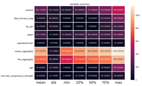
The database used shows the maximums and minimums of input and output components, as listed in Table 1. Figure 1 presents the statistical data of all components in the present data.

Figure 1: Statistics parameters of data

Table 1: Inputs and outputs: Maximum and Minimum

Model attributes	Values
	(Maximum)	(Minimum)
Cement (kg/m³)	540	102
Blast furnace slag (kg/m³)	359.4	0
Fly ash (kg/m³)	200.1	0
Water (kg/m³)	247	121.8
Superplasticizer (kg/m³)	32.2	0
Coarse aggregate (kg/m³)	1145	801
Fine aggregate(kg/m³)	992.6	594
Age (days)	365	1
Compressive strength of concrete (MPa)	82.6	2.33

It can be seen from the presented data that the database provided by Yeh [14] is quite consolidated and has a proper distribution for input and output variables. There are also several studies in the literature that use the same database, serving to perform a comparison between the results obtained in this study.

As the dataset has no null values, there is no need to attribute missing variables, nor are categorical variables found in this database. Thus, it was necessary to implement the feature scaling technique to standardize better the data used.

A visualization of histograms, density boxes, and box plots obtained from the database used is provided. As stated earlier, this visualization aims to give a better idea of which method is more appropriate to obtain the result.

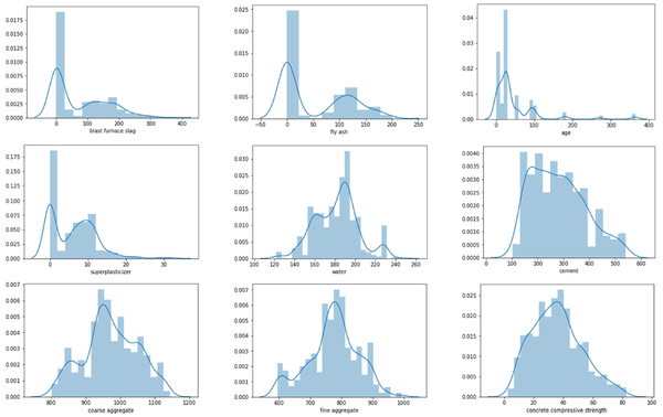
Figure 2 shows the histograms and density plots of the data used in the model. The variables have an almost normal distribution. Thus, it is possible to see that the efficiency of learning algorithms can be facilitated. It is important to note the maximum and minimum values of the compressive strength of concrete.

Figure 2: Histograms and density plots

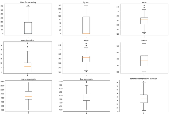
Figure 3 shows the box plots for the variables used. An analysis of the outlier values for each input and output variable was also performed, and the results are listed in Table 2. A proper distribution can be seen with no more than 10% of outliers in any attribute.

Figure 3: Box plot

Table 2: Analysis of outliers

Model attributes	Values
	(Number of outliers)	(Percentage of outliers)
Cement (kg/m³)	0	0.00
Blast furnace slag (kg/m³)	2	0.19
Fly ash (kg/m³)	0	0.00
Water (kg/m³)	9	0.87
Superplasticizer (kg/m³)	10	0.97
Coarse aggregate (kg/m³)	0	0.00
Fine aggregate(kg/m³)	5	0.49
Age (days)	59	5.73
Compressive strength of concrete (MPa)	4	0.39

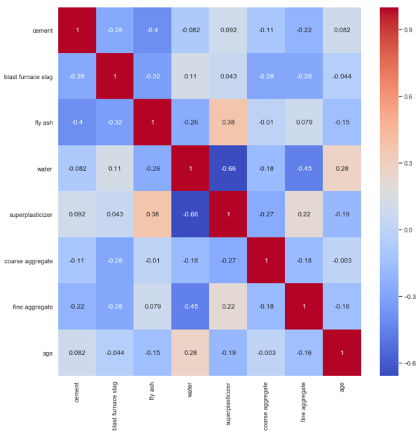
Figure 4 presents the correlation matrix of the data used in the model. The correlation matrix shows no correlation between the parameters used in the computational model. Therefore, it can be said that the components are mostly independent of each other.

Figure 4: Correlation matrix

With the data analysis presented in this unit, the adequate architecture of the computational models was developed and is presented in the following.

4.1. Random forest machine

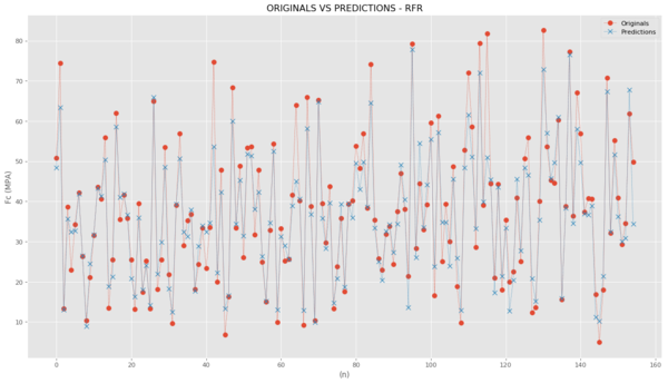
For the random forest machine learning model, the best parameters to be used in the kernel were defined. Figure 5 shows the original and predicted values for the random forest studied. The data related to the test portion were used. It can be seen that the model used presents an excellent result with the random forest. The value of R² is 0.90, and this model presents good results.

Figure 5: Original versus expected results for random forest

4.2. SVM

For the SVR learning model, the best parameters to be used in the kernel were defined. As GridsearchCV is used in this work to evaluate possible kernels, linear, polynomial, and RBFs could be applied. The intention was to evaluate the performance of these cores in the database presented and estimate different parameters of ε, which are the penalty parameters for the error. For polynomial and RBF kernels, there is also a kernel coefficient called the γ parameter. In such cases, there is a need to search these parameters to find the relationships between them and the best metrics that can optimally predict relevant results for the database.

By applying linear, polynomial, and RBFs, it was found that the RBF has been the best SVR kernel, which best predicts the results for the data presented. The best performance is evaluated based on the results of R². Thus, it is possible to evaluate the best performance of the model over different kernels, ε values, and γ parameters.

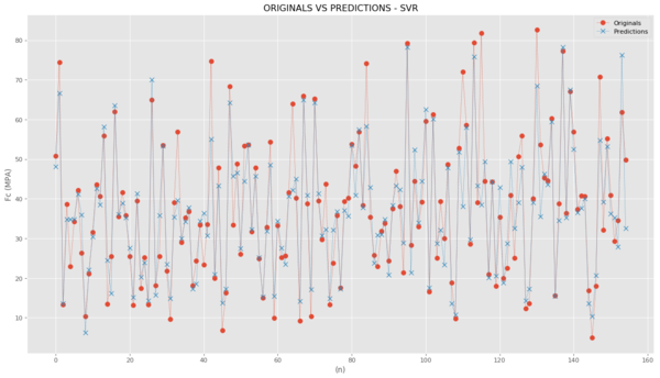
Figure 6 shows the original and predicted values for the SVR model studied. From results, it can be seen that RBF is the kernel that best fits the data used. This model found a value of R² = 0.82. The value of ε should not be too high, and this allows the model to override the data for higher penalties imposed on errors.

Figure 6: Original versus expected results for SVR

4.3. ANN

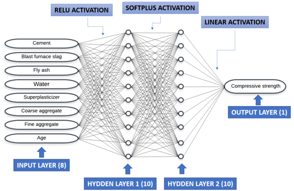
The model used Keras, an open-source neural network library available in Python. Keras was used on the TensorFlow backend [41,42]. The neural network was trained using the SGD optimizer. The defined architecture with the best result is presented, as can be seen in Figure 7.

Figure 7: Schematic representation of the ANN used

Eight neurons were used for the input layer. Further, 2 intermediate layers with 10 neurons each were used. One neuron was used in the output layer (the compressive strength of the concrete).

The activation functions for the initial and intermediate layers are ReLU. This decision was made based on its well-known performance for regression problems [39,40]. It was necessary to use a linear activation function in the last layer because the method is regression [43]. We used Glorot uniform to initialize the weights, with small numbers close to 0 [44].

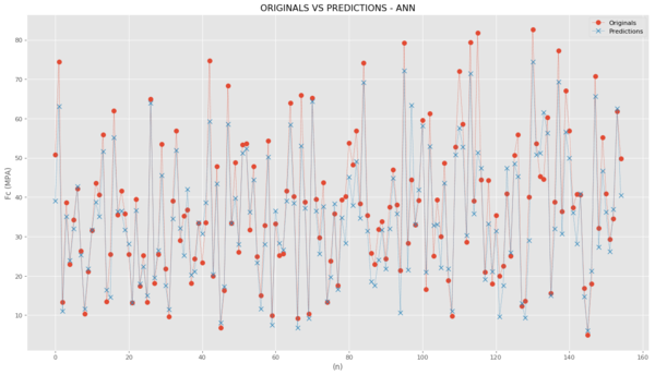
Figure 8shows the original and predicted values for the studied neural network. This result shows that the model used presents an excellent result with the given neural network. The value of R² = 0.90, and this model presents relatively good results.

Figure 8: Original versus expected results for ANN

The comparative results obtained in this study are present in Table 3.

Table 3: Comparison of obtained results

	RMSE	MAE	R²
Random forest	5.60	-	0.90
SVR	7.52	-	0.82
ANN	5.14	3.83	0.90

5. Conclusions

This work aimed to present the study of computational intelligence applied to define the concrete compressive strength from a database obtained in the studies of [14]. It was used three computational methods of machine learning and artificial intelligence: Random forests, support vector machines, and artificial neural networks. Data pre-processing and data visualization methods were also used to improve the results.

The obtained results show that the random forest gave the best performance (MSE = 5.60 and R² = 0.90) and average execution time. It can be noted that the support vector support method had the worst performance of the three used methods but presented the shortest execution time. Already, the artificial neural network showed the second-best result and the longest execution time. Table 4 presents a comparison between results obtained in this work, with results presented in the literature. It is possible to notice a good relation to the results obtained in this work.

Table 4: Comparison of the results obtained in this work with results previously predicted

Research	RMSE	MAE
ANN method (Yeh 2006 [14])	5.70	-
ANN method I (Gandomi and Alavi 2011 [45])	-	4.31
ANN method II (Gandomi and Alavi 2011 [45])	-	4.37
ANN method (Cook et al. 2019 [10])	6.33	5.04
SVR method (Cook et al. 2019 [10])	5.20	3.57
Random forest (Cook et al. 2019 [10])	3.27	4.51
ANN	5.14	3.83
SVR	7.52	-
Random Forest	5.60	-

The computational intelligence models used are reliable to solve different complex problems, such as prediction problems. These models can be used to solve a specific problem when a deviation in available data is expected and accepted, and also when a defined methodology is not available. Therefore, to predict the properties of concrete with high reliability, instead of using expensive experimental investigation, conventional and innovative models can be replaced by computational intelligence models.

Computational intelligence models can be used to predict the compressive strength of concrete specimens, as shown in this study. The prediction of mean percent error values for these simulations shows a high degree of consistency with compressive strength and is experimentally evaluated from the concrete specimens used. Thus, the present study suggests an alternative approach to evaluate compressive strength against destructive testing methods.

6. Acknowledgments

CAPES and CEFET-MG supported the work described in this paper.

7. References

[1] R. C. C. Hibbeler, Resistência dos Materiais, 7th ed. São Paulo, SP: Pearson, 2010.

[2] S. K. Babanajad, Application of genetic programming for uniaxial and multiaxial modeling of concrete. Switzerland: Springer, 2015.

[3] W.-F. Chen, Plasticity in reinforced concrete. J. Ross Publishing, 2007.

[4] B. Bresler and K. S. Pister, “Strength of concrete under combined stresses,” J. Proc., vol. 55, no. 9, pp. 321–345, 1958.

[5] D. C. Drucker and W. Prager, “Soil mechanics and plastic analysis or limit design,” Q. Appl. Math., vol. 10, no. 2, pp. 157–165, 1952.

[6] N. S. Ottosen, “A failure criterion for concrete,” Am. Soc. Civ. Eng. Eng. Mech. Div. J., vol. 103, no. 4, pp. 527–535, 1977.

[7] N. D. Hoang, X. L. Tran, C. H. Le, and D. T. Nguyen, “A backpropagation artificial neural network software program for data classification in civil engineering developed in . NET framework,” DTU J. Sci. Technol., vol. 03, no. 34, pp. 51–56, 2019.

[8] U. Reuter, A. Sultan, and D. S. Reischl, “A comparative study of machine learning approaches for modeling concrete failure surfaces,” Adv. Eng. Softw., vol. 116, no. July 2017, pp. 67–79, 2018.

[9] A. A. Torky and A. A. Aburawwash, “A Deep Learning Approach to Automated Structural Engineering of Prestressed Members,” Int. J. Struct. Civ. Eng., vol. 7, no. 4, pp. 347–352, 2018.

[10] R. Cook, J. Lapeyre, H. Ma, and A. Kumar, “Prediction of Compressive Strength of Concrete: Critical Comparison of Performance of a Hybrid Machine Learning Model with Standalone Models,” J. Mater. Civ. Eng., vol. 31, no. 11, pp. 1–15, 2019.

[11] Z. Sun, K. Li, and Z. Li, “Prediction of concrete compressive strength based on principal component analysis and radial basis function neural network Prediction of concrete compressive strength based on principal component analysis and radial basis function neural network,” IOP Conf. Ser. Mater. Sci. Eng., 2019.

[12] P. G. Asteris, “Concrete compressive strength using artificial neural networks,” Neural Comput. Appl., vol. 2, 2019.

[13] R. Rajeshwari and S. Mandal, “Prediction of compressive strength of high-volume fly ash concrete using artificial neural network,” Lect. Notes Civ. Eng., vol. 25, pp. 471–483, 2019.

[14] I.-C. Yeh, “Analysis of Strength of Concrete Using Design of Experiments and Neural Networks,” J. Mater. Civ. Eng., vol. 18, no. 4, pp. 597–604, 2006.

[15] D. W. Scott, “On optimal and data-based histograms,” Biometrika, vol. 66, no. 3, pp. 605–610, 1979.

[16] J. H. Steiger, “Tests for comparing elements of a correlation matrix,” Psychol. Bull., vol. 87, no. 2, p. 245, 1980.

[17] L. Wang, G. Wang, and C. A. Alexander, “Big data and visualization: methods, challenges and technology progress,” Digit. Technol., vol. 1, no. 1, pp. 33–38, 2015.

[18] G. Forman, “BNS feature scaling: an improved representation over tf-idf for svm text classification,” in Proceedings of the 17th ACM conference on Information and knowledge management, 2008, pp. 263–270.

[19] M.-L. Zhang and Z.-H. Zhou, “Improve multi-instance neural networks through feature selection,” Neural Process. Lett., vol. 19, no. 1, pp. 1–10, 2004.

[20] B. Efron and R. Tibshirani, “Improvements on cross-validation: the 632+ bootstrap method,” J. Am. Stat. Assoc., vol. 92, no. 438, pp. 548–560, 1997.

[21] G. H. Golub, M. Heath, and G. Wahba, “Generalized cross-validation as a method for choosing a good ridge parameter,” Technometrics, vol. 21, no. 2, pp. 215–223, 1979.

[22] J. Shao, “Linear model selection by cross-validation,” J. Am. Stat. Assoc., vol. 88, no. 422, pp. 486–494, 1993.

[23] L. Buitinck et al., “API design for machine learning software: experiences from the scikit-learn project”, 2013.

[24] F. Pedregosa et al., “Scikit-learn: Machine learning in Python,” J. Mach. Learn. Res., vol. 12, no. Oct, 2011.

[25] I. Barandiaran and T. K. Ho, “The Random Subspace Method for Constructing Decision Forest,” IEEE Trans. Pattern Anal. Mach. Intell, vol. 20, no. 8, pp. 832–844, 1998.

[26] M. Pal, “Random forest classifier for remote sensing classification,” Int. J. Remote Sens., vol. 26, no. 1, pp. 217–222, 2005.

[27] P. O. Gislason, J. A. Benediktsson, and J. R. Sveinsson, “Random forests for land cover classification,” Pattern Recognit. Lett., vol. 27, no. 4, pp. 294–300, 2006.

[28] L. Breiman, “Random forests,” Mach. Learn., vol. 45, no. 1, pp. 5–32, 2001.

[29] C.-F. Lin and S.-D. Wang, “Fuzzy support vector machines,” IEEE Trans. neural networks, vol. 13, no. 2, pp. 464–471, 2002.

[30] B. Scholkopf and A. J. Smola, “Learning with kernels: support vector machines, regularization, optimization, and beyond,” IEEE Trans. Neural Networks, vol. 16, no. 3, pp. 781–781, 2001.

[31] J. A. K. Suykens and J. Vandewalle, “Least squares support vector machine classifiers,” Neural Process. Lett., vol. 9, no. 3, pp. 293–300, 1999.

[32] H. Drucker, C. J. C. Burges, L. Kaufman, A. J. Smola, and V. Vapnik, “Support vector regression machines,” in Advances in neural information processing systems, 1997, pp. 155–161.

[33] S. R. Gunn, “Support vector machines for classification and regression,” ISIS Tech. Rep., vol. 14, no. 1, pp. 5–16, 1998.

[34] D. Basak, S. Pal, and D. C. Patranabis, “Support vector regression,” Neural Inf. Process. Rev., vol. 11, no. 10, pp. 203–224, 2007.

[35] J. J. Hopfield, “Artificial neural networks,” IEEE Circuits Devices Mag., vol. 4, no. 5, pp. 3–10, 1988.

[36] W. S. Sarle, “Neural networks and statistical models,” Proc. Ninet. Annu. SAS Users Gr. Int. Conf., 1994.

[37] A. Gulli and S. Pal, Deep Learning with Keras. Packt Publishing Ltd, 2017.

[38] V. F. Arruda, G. F. Moita, and P. F. S. Silva, “Determining the optimal artificial neural network architecture capable of predict the compressive strength of concrete,” Proc. XL Ibero-Latin-American Congr. Comput. Methods Eng., 2019.

[39] D. A. Clevert, T. Unterthiner, and S. Hochreiter, “Fast and accurate deep network learning by exponential linear units (ELUs),” 4th Int. Conf. Learn. Represent. ICLR 2016 - Conf. Track Proc., pp. 1–14, 2016.

[40] G. Klambauer, T. Unterthiner, A. Mayr, and S. Hochreiter, “Self-normalizing neural networks,” Adv. Neural Inf. Process. Syst., vol. 2017-Decem, pp. 972–981, 2017.

[41] P. Goldsborough, “A tour of tensorflow”, 2016.

[42] J. Kossaifi, Y. Panagakis, A. Anandkumar, and M. Pantic, “Tensorly: Tensor learning in python,” J. Mach. Learn. Res., vol. 20, no. 1, pp. 925–930, 2019.

[43] A. F. Agarap, “Deep learning using rectified linear units (relu),” arXiv Prepr. arXiv1803.08375, 2018.

[44] A. Kaveh, M. Kalateh-Ahani, and M. Fahimi-Farzam, “Constructability optimal design of reinforced concrete retaining walls using a multi-objective genetic algorithm,” Struct. Eng. Mech., vol. 47, no. 2, pp. 227–245, 2013.

[45] A. H. Gandomi and A. H. Alavi, “Applications of computational intelligence in behavior simulation of concrete materials,” Stud. Comput. Intell., vol. 359, pp. 221–243, 2011.