Study of the aerodynamic forces on a simplified shape X-43 aircraft under supersonic conditions, design optimization

Abstract

The paper focuses on the shape optimization, based on the resultant aerodynamic forces, of a simplified X-43 aircraft. The equations of oblique shock waves and Prandtl-Meyer expansion waves, along with the improvement of the aircraft geometry using a genetic algorithm optimisation, will allow to shape and optimize the external dimensions of the bi-dimensional simplified aircraft design. The main purpose of the optimisation is the reduction of the drag force while maintaining a sufficient lift to hold the weight of the aircraft. The optimization is undertaken at four different altitudes, obtaining for each altitude the most favourable aircraft shape to maximize the aircraft efficiency. The study can be extended to various possible aircraft weight configurations.

Keywords: X-43, simulation Computational Fluid Dynamics (CFD), hypersonics, aerodynamic shape optimization, generic algorithms

1 Introduction

The aerospace industry is very demanding in terms of high performance, this is the reason why, optimisation techniques are particularly welcome in order to find the best design for each given situation. Optimisation algorithms allow improving new designs or designs already created, without the need of testing a large number of possible configurations.

Hypersonic flight vehicles such as the X-43, require profound studies on each technological part. Examples of the depth of such studies are, the optimization of the internal engine flow channel via employing genetic algorithms, which was undertaken by [1]. Aeroelastic and aerothermoelastic-acoustics simulations based on new computational Fluid Mechanics models, were presented in [2,3]. The pressure distribution over this particular aircraft was numerically determined by [4], where they implemented a method which introduced artificial dissipation coefficients. The resulting overall lift and drag coefficients for several angles of attack were obtained when solving the three dimensional Navier-Stokes equations by [5,6], the comparison with the experimental measurements gave a very good agreement. The flight dynamics affecting a 2D hypersonic vehicle resembling the X-43, were described in [7], where the non linear equations of motion were derived. An increase of the aerodynamic efficiency of the hypersonic aircraft (HA) was obtained in [8], via adding energy in front of the bow of the HA. It was observed that the addition of energy weakened the shock wave. In [9], the shock-wave structures appearing around the same (HA) studied by the rest of the researchers cited in this paper, were filmed using a high-speed video camera. Visualizations of the flow at the engine entrance throat, where the shock waves reflect, were particularly interesting.

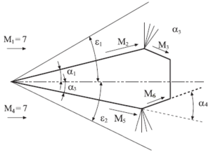
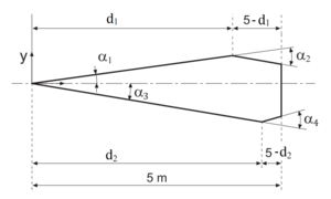
In the present study, given the Mach number and the altitude at which the X-43 simplified shape aircraft performs, the aerodynamic forces acting on the aircraft will be calculated based on the mathematical formulation defined in section II. In the next step, these forces will be optimized, computing this formulation with a python code and using the RMOP optimizer (http://tts.cimne.com/rmop). The optimization will be based on the variation of the main geometrical parameters of the aircraft, presented in Figures 1 and 2. The shape of the chosen aircraft, was as well optimised for different possible flight altitudes and Mach numbers.

2 Mathematical model

In the present section, the required equations able to determine the lift and drag of the simplified shape X-43 aircraft, for a given initial geometry, free-stream Mach number and for a certain altitude, will be introduced. Further information regarding the equations development is to be found in [10,11,12]. It has to be noted that oblique reattached shock waves will appear at the leading edge. Expansion waves will appear both in extrados and intrados of the aerodynamic body. Figure 1 shows graphically the main features of the problem under study.

Figure 1. Oblique shock waves and Prandtl-Meyer expansion waves on a simplified shape of the X-43

Since the objective is to determine the aerodynamic forces, it is needed to calculate the pressure on each aircraft surface. In order to obtain the pressure, it is first required to calculate the different Mach numbers, therefore, it will be necessary to study the change on velocity through the oblique shock wave and expansion Prandtl-Meyer waves.

It has to be noted that the procedure used to calculate the forces acting on the extrados and intrados of the aircraft is identical. This is why the following explanation will focus on the extrados part of the airplane.

The procedure followed to calculate the Mach number after the shock wave ${\textstyle M_{2}}$, starts by finding the oblique shock wave angle ${\textstyle \varepsilon _{1}}$. This angle can be found from the wedge inclination angle ${\textstyle \alpha _{1}}$ and the free-stream Mach number ${\textstyle M_{\infty }=M_{1}}$, as the implicit equation (1) shows

${\frac {1}{\tan \alpha _{1}}}={\bigg [}{\frac {\gamma +1}{2}}{\bigg (}{\frac {M_{1}^{2}}{M_{1}^{2}\sin ^{2}\varepsilon _{1}-1}}{\bigg )}-1{\bigg ]}\tan \varepsilon _{1}$

(1)

To obtain the Mach number ${\textstyle M_{2}}$ after the oblique shock wave, initially equation (2) is required. From this equation, the upstream Mach number perpendicular to the oblique shock wave ${\textstyle M_{N1}}$ is gathered. The downstream Mach number perpendicular to the shock wave, ${\textstyle M_{N2}}$, is to be obtained from equation (3). Notice that from this equation two normal Mach numbers will be obtained, the subsonic one is the one required for the next step. Via introducing the normal subsonic Mach number obtained in the previous step, ${\textstyle M_{N2}}$ in equation (4), the downstream Mach number ${\textstyle M_{2}}$ is obtained

$M_{1}={\frac {M_{N1}}{\sin \varepsilon _{1}}}$

(2)

$M_{N1}^{2}={\frac {M_{N2}^{2}+{\big (}{\frac {2}{\gamma -1}}{\big )}}{{\big (}{\frac {2\gamma }{\gamma -1}}{\big )}M_{N2}^{2}-1}}$

(3)

$M_{N2}=M_{2}\sin \varepsilon _{1}$

(4)

This final result ${\textstyle M_{2}}$, is the starting point to calculate the Mach number after the expansion waves ${\textstyle M_{3}}$. In this case, the procedure is based on initially finding a required angle ${\textstyle \eta _{0}}$, needed to obtain a downstream Mach number ${\textstyle M_{2}}$, and whenever the upstream Mach number is equal to one. Equation (5) is meant to be used to obtain this initial angle

${\begin{array}{cc}\eta _{0}={\sqrt {\frac {\gamma {+1}}{\gamma {-1}}}}\tan ^{-1}({\sqrt {\frac {\gamma {-1}}{\gamma {+1}}}}B)-\tan ^{-1}(B)\\\end{array}}$

(5)

where ${\textstyle B={\sqrt {M_{2}^{2}-1}}}$.

Since equation (5) can just be employed when the upstream Mach number is the unity, the flow will need to turn an angle ${\textstyle \eta }$ to obtain a downstream Mach number ${\textstyle M_{3}}$, the angle ${\textstyle \eta }$ will be ${\textstyle \eta =\eta _{0}+\alpha _{2}}$. Now, by substituting in equation (5) the value of ${\textstyle \eta }$ just obtained, the Mach number ${\textstyle M_{3}}$ will be the remaining variable to be determined. Two values of ${\textstyle M_{3}}$ will be obtained from equation (5), the supersonic one is to be the one required. The same procedure is to be employed in the intrados part of the vehicle in order to obtain the Mach numbers ${\textstyle M_{5}}$ and ${\textstyle M_{6}}$.

Finally, the pressure existing after the extrados oblique shock wave ${\textstyle P_{2}}$ and after the Prandl-Meyer expansion waves ${\textstyle P_{3}}$, can be determined from equations (6) and (7), respectively. The same procedure is to be used to calculate the pressures acting on the surfaces 5 and 6. The force acting perpendicularly to each surface is simply the pressure multiplied by the area, the projection of the forces in x and y direction will give the drag and lift forces respectively

${\frac {P_{2}}{P_{1}}}={\frac {2\gamma }{\gamma +1}}M_{N1}^{2}-{\frac {\gamma {-1}}{\gamma {+1}}}$

(6)

${\frac {P_{3}}{P_{2}}}={\frac {{\bigg (}1+{\frac {\gamma -1}{2}}M_{2}^{2}{\bigg )}^{\frac {\gamma }{\gamma {-1}}}}{{\bigg (}1+{\frac {\gamma -1}{2}}M_{3}^{2}{\bigg )}^{\frac {\gamma }{\gamma {-1}}}}}$

(7)

3 Optimisation model

For the optimization it has been used the Robust Multi-Objective Optimization Platform RMOP, a platform based on genetic algorithms and evolutionary strategies, which is the CIMNE's in-house optimization tool. It implements a Genetic Algorithm based on ${\textstyle \lambda }$ - ${\textstyle \mu }$ strategy and Particle Swarm Optimization method, with soft coupling and Gradient-based techniques, like Conjugate Gradient or Newton methods, just to mention two of them. Among the techniques to enhance the convergence and accuracy of the analysis, it implements Nash Games, and Hybrid Games, as well as hybridization through the genetic operators. The most relevant one is the Nash Games. It provides an improvement of convergence through the definition of what is called players. Each player is taking care of part of the problem (some of the design variables and/or objective functions), defining a competition between players that push the optimization further. The hybridization can be completed with the definition of a Pareto player, which is solving the complete problem. The platform is also enabling a pure hybrid approach. Two or more populations can be defined, assigning exploration and exploitation roles to each of them. The roles can be defined through the values of the probability of cross-over and mutation, or through the assignment of different objective functions and constraint to each population. Hybridization through the combination of optimization methods, as well as the mixing between multiple populations and combination of methods is an on-going development of the platform. For this analysis, standard GA has been used.

The changing inputs of the optimization are the design variables. These are the four angles defining the aircraft geometry, ${\textstyle \alpha _{1}}$, ${\textstyle \alpha _{2}}$, ${\textstyle \alpha _{3}}$ and ${\textstyle \alpha _{4}}$, and the dimensions ${\textstyle d_{1}}$ and ${\textstyle d_{2}}$, as shown in Figure 2.

Figure 2. Design variables on the simplified shape of the X-43

During the optimization, these variables are chosen within a range due to geometrical requirements, as for instance having sufficient space for a possible rear engine. The range in which each variable can be selected and the changing step between the bounds are represented in Table 1.

Table 1. Design variables bounds and step

	Lower limit	Upper limit	Variable step
$\alpha _{1}$, ${\textstyle \alpha _{3}}$	7	24	0.1
$\alpha _{2}$, ${\textstyle \alpha _{4}}$	0	40	0.1
$d_{1}$, ${\textstyle d_{2}}$	4.2	4.95	0.05

The objective function is the best solution or group of solutions that the model aims to find, this objective function is, in this case, to be minimised. Having a multi-objective optimisation platform, more than one objective function can be established. The optimisation has been performed in order to reduce the drag force and increase the lift force which has to compensate the weight of the aircraft.

The purpose is obtaining a design curve of the minimum drag and maximum lift forces for different configurations. The main interest in the optimisation is reducing the drag force, as it will involve a decrease of the power required. However, it is also interesting to evaluate the lift force providing design configurations that can lift higher or lower weight values of the aircraft.

As the optimisation is based in minimising the parameters, and the lift force is wanted to increase, the optimisation will found the minimum negative values of the lift force ($-L$), finding in this way the maximum values.

Having defined the design variables and the objective functions, the optimisation case can be formulated as

$D:\chi \rightarrow R\quad min(D(\alpha _{1},\alpha _{2},\alpha _{3},\alpha _{4}<,d_{1},d_{2}))$

$D:\chi \rightarrow R\quad min(L(\alpha _{1},\alpha _{2},\alpha _{3},\alpha _{4}<,d_{1},d_{2}))$

$\alpha _{1}\in \chi _{1}$ $\alpha _{2}\in \chi _{2}$ $\alpha _{3}\in \chi _{3}$ $\alpha _{4}\in \chi _{4}$

$d_{1}\in \chi _{5}$ $d_{2}\in \chi _{6}$

where $\chi _{1},\chi _{3}=[7,24]$; $\chi _{2},\chi _{4}=[0,40]$ and $\chi _{5},\chi _{6}=[4.2,4.95]$.

The optimisation was run with a population of 100 individuals for 5000 evaluations, with a random initial population of 200 individuals, a 0.9 probability of crossover and a 0.1 probability of mutation.

4 Results

The conditions at which the aircraft was initially optimised were, ${\textstyle Mach=7}$ and a flight altitude of ${\textstyle h=30000m}$. Following the International Standard Atmosphere (ISA), the thermo-physical values were obtained; a temperature of ${\textstyle T=226.65K}$, a pressure of ${\textstyle P=1171.87Pa}$ and a gravity of ${\textstyle g=9.715m/s^{2}}$. In reality the optimization was undertaken at another three different altitudes, 25000 m, 35000 m and 40000 m. Table 2 presents the air properties at all studied altitudes.

Table 2. ISA Atmosphere

Altitude [m]	Temperature [K]	Pressure [Pa]
25000.0	221.650	2511.02
30000.0	226.650	1171.87
35000.0	237.050	558.924
40000.0	251.050	277.522
Density [kg/m3]	Sound speed [m/s]	Viscosity [Pa.s]
0.0394658	298.455	0.0000146044
0.0180119	301.803	0.0000148835
0.00821392	308.649	0.0000154559
0.00385101	317.633	0.0000162096

It is important to remember that the results of a multi-objective optimisation do not have a unique solution, as there is no solution that optimises each objective function at the same time. This is why, a set of equally good solutions is encountered called the Pareto front. These are also called non-dominated solutions as they dominate all the other solutions except the ones in the Pareto.

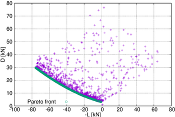
The resultant Pareto of the optimisation is shown in Figure 3, together with the evolution of the different attempts to find the optimum values. It can be easily seen that a high number of attempts are close to the optimum results.

Figure 3. Pareto front of the optimisation

From the Pareto front configurations a range of values can be immediately discarded due to the incapacity of lifting the minimum weight necessary to build the aircraft. The weight of the real X-43 NASA aircraft is 1400 kg, so the results for lift values below 14kN can be discarded. However, having this weight reduced would imply the possibility of having configurations with lower values of drag, as can be seen on Figure 3.

Some of the design variables which conform the Pareto front with a possible optimum performance are presented in Table 3. These parameters define the optimum geometries of the aircraft for the given objective functions. The total number of configurations obtained on the Pareto front is 420, therefore, the table just represents a overview of the optimum designs.

Table 3. Some of the design variables optimised values, taken from the Pareto front

${\boldsymbol {\alpha _{1}}}^{[\circ ]}$	${\boldsymbol {\alpha _{2}}}^{[\circ ]}$	${\boldsymbol {\alpha _{3}}}^{[\circ ]}$	${\boldsymbol {\alpha _{4}}}^{[\circ ]}$	${\boldsymbol {d_{1}}}[m]$	${\boldsymbol {d_{2}}}[m]$
7.0	2.6	10.6	0.0	4.6	4.2
L = 10492 [N]			D = 5342 [N]
7.0	8.8	13.8	0.0	4.55	4.2
L = 22708 [N]			D = 8449 [N]
7.0	3.7	15.7	0.0	4.4	4.2
L = 30649 [N]			D = 10772 [N]
7.0	8.1	17.8	0.0	4.6	4.2
L = 40754 [N]			D = 14390 [N]
7.0	5.8	19.7	0.0	4.55	4.2
L = 50624 [N]			D = 18204 [N]
7.0	3.9	21.4	0.0	4.55	4.2
L = 60018 [N]			D = 22275 [N]
7.0	4.1	23.1	0.0	4.5	4.2
L = 70406 [N]			D = 27038 [N]
7.0	9.1	23.9	0.0	4.6	4.2
L = 75733 [N]			D = 29645 [N]

From Table 3 it can be seen that there are some parameters that remain constant on the Pareto front, these are the angles ${\textstyle \alpha _{1}}$ with ${\textstyle 7^{\circ }}$, ${\textstyle \alpha _{4}}$ with ${\textstyle 0^{\circ }}$ and the distance ${\textstyle d_{2}}$ with ${\textstyle 4.2m}$. It has to be noted that the three design variables have acquired the value of their lower bound, which have been set in order to have sufficient space for the engine to be located at the rear.

This entails that it is needed the thinnest possible surface on the extrados part of the aircraft implying the lowest value possible for ${\textstyle \alpha _{1}}$, which is ${\textstyle 7^{\circ }}$. Besides, the distance ${\textstyle d_{1}}$ is around 4.55${\textstyle m}$ and together with ${\textstyle \alpha _{2}}$ fulfills the sufficient space for the engine. In the intrados region, it is relevant to highlight the null value of ${\textstyle \alpha _{4}}$, which is due to the elimination of the expansion waves, these expansion waves increase the drag due to the particularly low pressure generated downstream of the expansion wave.

Regarding the parameters that do change, the angle ${\textstyle \alpha _{3}}$ changes directly with the aerodynamic forces. The angle increases from ${\textstyle 7^{\circ }}$ up to ${\textstyle 23.9^{\circ }}$ and the drag and lift forces increase along with it. It can be said that it has a high influence on the vehicle overall performance.

On the other side, the angle ${\textstyle \alpha _{2}}$ and the distance ${\textstyle d_{1}}$ have multiple values for different optimum configurations that go from ${\textstyle 0.6^{\circ }}$ until ${\textstyle 13^{\circ }}$, and from ${\textstyle 4.5m}$ to ${\textstyle 4.6m}$, respectively.

• Altitudes discussion

It is of interest to evaluate the aerodynamic forces of the aircraft for different altitudes, since the density and pressure of the air plays a predominant role.

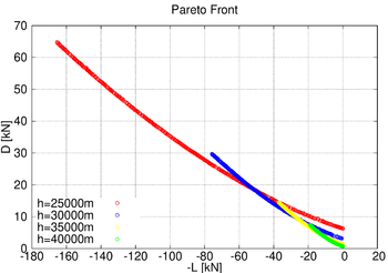
Figure 4. Pareto front for different altitudes

In Figure 4 the resulting Pareto front is shown for four optimisations at different altitudes (25, 30, 35 and 40 km). The considerable difference between diverse altitudes is highly noted regarding the range of values of the aerodynamic forces lift and drag, while all the Pareto fronts tend to a similar curve.

These highly different ranges of aerodynamic forces are caused by the difference of pressure between altitudes. As can be observed in Figure 4, for lower altitudes the range of lift and drag forces that can be achieved changing the geometry is much higher than with altitudes above. This is a consequence of the effect that changing the geometry has on the variation of pressures around the aircraft, at higher altitudes this effect is lower than in lower altitudes and, for this reason, the impact on the aerodynamic forces is different. As the altitude is increased, the values of drag are decreased considerably along with the lift force. The maximum value of lift force that can be obtained changing the geometry at an altitude of $h=40000m$ is around 20kN while flying at $h=25000m$ is around 165kN, the same happens with the minimum drag force being 0.7kN at $h=40000m$ and 6.3kN at $h=25000m$.

Having a look to the design variables for each altitude, similar solutions have resulted in terms of geometry for the optimum conditions, hence, nearly the same design configurations of the aircraft are optimum for different altitudes. However, as said, it has different impact on the aerodynamic forces.

• Velocity and power

The viability of the flight can be discussed from the engine power needed for each altitude. In Table 4 the power needed for a specific range of drag from the Pareto curve is shown for each altitude.

Table 4

$h[m]$	$D[kN]$	$v[m/s]$	$P[MW]$
10000	86.5-886.8	2096.5	181.3-1859.2
25000	6.3-64.7	2088.5	13.0-133.63
30000	3.2-29.6	2135.6	6.8-63.2
35000	1.4-14.5	2203.4	3.1-31.9
40000	0.7-7.4	2269.2	1.6-16.8

On the first column of Table 4 are shown the different altitudes at which the optimisation has been run, it has to be noted that it has also been run the optimisation for a 10km altitude but it has not been shown on the Figure 4. This is due to the non viability of the aircraft at this altitude, as it will be seen on the power needed. On the second column it can be seen the range of different drag forces that can be achieved modifying the geometry as seen on Figure 4. The third column of the Table shows the velocity at which the aircraft is flying, considering that the Mach number is 7, as mentioned before. Finally, on the last column are displayed the range of values of the power needed obtained from the drag force and the velocity.

These values approximate the order of magnitude of the power that would be needed at each altitude, it has to be noted that it changes drastically for different altitudes, having the lowest values at the highest altitudes as it happens with the drag force.

It is of common knowledge that Ramjets and Scramjets are able to generate a power around 100 MW, thus, when comparing with Table 4, it can be concluded that the viability of the flight is acceptable from 25 km of altitude and above, requiring an additional transport for the aircraft to this altitude, as at 10 km the engine can not supply the power needed. Nevertheless, newer technology is likely to improve the power supplied by these engines.

5. Conclusions

With the mathematical model developed, coded into Python and joined with an optimisation algorithm it is resulted a design curve of different aerodynamic forces changing the geometry of the aircraft. It is obtained for each one of these force values a not intuitive configuration of the design variables, being able to add restrictions or dependencies between the variables, building a complex design with few computational resources and time.

The simulations have been done with a conventional laptop with 8 cores. Each iteration has a duration time of around 1 second, and it has been done a number of 5000 simulations parallelised, resulting in a duration of 15 minutes for each optimisation.

The optimisation of 6 design variables has resulted in fixing 3 of these 6 design variables in their lower bound values searching for a thin aircraft and limited by the engine space and minimum thickness of the aircraft. Hence, the design curve of the geometry is obtained varying only the values of ${\textstyle \alpha _{2}}$, ${\textstyle \alpha _{3}}$ and ${\textstyle d_{1}}$. As the lift force has to be sufficient to lift the weight of the aircraft, the results on the Pareto front below a lift force of 14kN (weight of actual NASA X-43) have been discarded.

Moreover, the results have been later extrapolated to different altitudes in order to study the performance of the aircraft in the different stages of the flight, considering the required power for each altitude and each design configuration. The results have shown that different altitudes affect highly to the resulting aerodynamic forces when changing the geometry, due to the pressure difference. The drag and lift decrease as the altitude increases, therefore allowing to have a lower required power at higher altitudes.

This optimisation process allows a much more easy way of designing with a wide range of parameters to take into account in order to achieve the optimum conditions. However, in this case, some of the parameters that have been optimised have resulted optimum in their boundary values. Is for this reason that further optimisations could be done modifying the geometry with a more complex one together with wider limits.

References

[1] Ahuja V., Hartfield R.J., Shelton A. Optimization of hypersonic aircraft using genetic algorithms. Applied Mathematics and Computation, 242:423–434, 2014.

[2] Gupta K.K., Voelker L.S. Aeroelastic simulation of hypersonic flight vehicles. AIAA Journal, 50(3):717–723, 2012.

[3] Gupta K.K., Choi S.B., Lung S.F., Ibrahim A. Aerothermoelastic-acoustics simulation of flight vehicles. American Institute of Aeronautics and Astronautics, AIAA Journal, 55(1):49–56, 2016.

[4] Elizarova T.G., Shirokov I.A. Artificial dissipation coefficients in regularized equations of supersonic aerodynamics. Doklady Mathematics, 98(3):648–651, 2018.

[5] Zheleznyakova A.L., Surzhikov S.T. Application of the method of splitting by physical processes for the computation of a hypersonic flow over an aircraft model of complex configuration. High Temperature, 51(6):816–829, 2013.

[6] Zheleznyakova A.L., Surzhikov S.T. Calculation of a hypersonic flow over bodies of complex configuration on unstructured tetrahedral meshes using the AUSM scheme. High Temperature, 52(2):271–281, 2014.

[7] Mirmirani M., Kuipers M., Levin J., Clark A.D. Flight dynamic characteristics of a scramjet-powered generic hypersonic vehicle. IEEE, 2009 American Control Conference, 2525–2532, 2009.

[8] Khankhasaeva Y.V., Borisov V.E., Lutsky A.E. Influence of energy input on the flow past hypersonic aircraft X-43. Journal of Physics: Conference Series, 815(1):012018, 2017.

[9] Kotov M.A., Ruleva L.B., Solodovnikov S.I., Surzhikov S.T. Preliminary experimental assessment of supersonic airflow behavior over ExoMars and X–43 inlet models using multiple flow regime shock tube. Journal of Physics: Conference Series, 1009(1):012038, 2018.

[10] Zucrow M.J., Hoffman J.D. Gas dynamics. Vol. 1, Wiley, 1976.

[11] Anderson J.D. Modern compressible flow: with historical perspective. Vol. 12, McGraw-Hill, New York, 1990.

[12] Bergada J.M. Mecánica de fluidos: breve introducción teórica con problemas resueltos. Iniciativa Digital Politecnica, Oficina de Publicacions Academiques Digitals, 2017.