Revision as of 03:38, 29 October 2024 (view source) Huanglh (talk | contribs) m (Huanglh moved page Draft Huang 935701954 to Chenhan Huang 2024a) ← Older edit		Revision as of 05:33, 29 October 2024 (view source) Huanglh (talk | contribs) Newer edit →
Line 24:		Line 24:
	==1 Background of the study==		==1 Background of the study==
−
−	Climate change is a global challenge, with greenhouse gas emissions leading to rising global temperatures and frequent extreme weather events. The power sector is one of the major sources of global carbon emissions, and achieving carbon peak and carbon neutrality in this sector is a key initiative for countries to fulfill their commitments under international climate conventions such as the Paris Agreement. For example, China has proposed a "dual-carbon" goal, where the low-carbon transformation of the power sector has far-reaching implications for global climate governance, demonstrating the responsibility of a major country. [1] The power sector's low-carbon transition not only demonstrates the responsibility of a major power but also helps to promote a common global response to climate change. Reducing carbon emissions from the power sector can directly decrease the growth rate of greenhouse gases such as sulfur dioxide, nitrogen oxides, and particulate matter in the atmosphere, which are among the main causes of environmental problems like acid rain and haze.
−
−	Utilizing the electricity-carbon model, it is possible to accurately assess the carbon emissions of different power generation technologies (e.g., traditional coal power generation, natural gas power generation, and emerging solar power generation, wind power generation, nuclear power generation, etc.) at various stages. Through detailed data analysis, it is possible to determine when and at what rate to phase out high-carbon emitting power generation technologies, while simultaneously vigorously developing low-carbon or zero-carbon power generation technologies. For example, the electricity-carbon model can simulate that over the next 10-20 years, if carbon peaking is to be achieved, the installed capacity of solar and wind power generation will need to be expanded at a certain growth rate per year, while gradually reducing the operating hours of thermal power units. This will help the power industry to formulate a scientific and reasonable energy transition strategy, avoiding blind investment and resource wastage.At the same time, the electricity-carbon model can take into account the real-time operation of the power system, including changes in load demand and the generation characteristics of different power sources. On the premise of ensuring the reliability of power supply, optimized scheduling through the model can prioritize the use of low-carbon emission power sources for power generation. Additionally, the government and enterprises will introduce various policies and technical measures to promote carbon peaking and carbon neutrality, such as carbon tax policies, renewable energy subsidy policies, and the promotion of carbon capture, utilization, and storage (CCUS) technology. The electricity-carbon model can quantitatively assess these policies and technical measures. The results from the model can serve as a scientific basis to demonstrate to the public, investors, and the international community the specific action plans and progress of the power industry in addressing climate change. Transparent quantitative analysis of carbon emissions and planning of emission reduction pathways can enhance social confidence in the low-carbon transformation of the power industry and provide strong data support for international climate negotiations, proving the actual contributions made by the country or region in the field of electricity to combat climate change.
−
−	Estimation and management of carbon emissions has become a key issue in scientific research and policy development[2]. The Carbon emission estimation modeling, as a major tool for assessing and predicting corporate carbon emissions, plays a crucial role in formulating emission reduction strategies and achieving carbon neutrality goals[3,4]. electricity-carbon model, also known as "electric-carbon analysis model" or "electric-carbon calculation model", is based on the correlation between electricity consumption and carbon emissions from consumption of other energy varieties and industrial production, and makes use of the advantages of electricity big data, such as wide coverage, real-time, high resolution and high degree of digitization, to construct an innovative model to estimate the carbon emissions of enterprises. It is based on the correlation between electricity consumption and carbon emissions from other energy sources and industrial production, and utilizes the advantages of wide coverage, strong real-time, high resolution and high degree of digitization of big data of electricity to innovatively construct the calculation method of "electricity-carbon calculation"[5]. The electric power industry is a major concern for the nation's economy and people's livelihood. The power industry is a basic energy industry that has a major impact on the people's livelihood and national security, and power consumption is also an indicator of carbon dioxide emissions，The electricity consumption is also an indicator of carbon dioxide emissions[6]. Therefore, the development of enterprise "electricity-carbon model", the use of accurate measurement of electricity, real-time access, unified management and other characteristics of the carbon dioxide emissions of emission-control enterprises accurate prediction, real-time and effective mapping of the province's carbon assets, carbon emissions, is not only conducive to enriching the means of carbon regulation, but also conducive to the provision of a reference basis for the prediction of the carbon price, which will help local enterprises to better participate in the national carbon market transactions. It not only helps to enrich the means of carbon regulation, but also helps to provide a reference basis for carbon price prediction, which in turn helps local enterprises better participate in the national carbon market. Accurate carbon emission estimation not only helps the government and enterprises to formulate more scientific and reasonable emission reduction strategies and policies, but also lays a solid foundation for realizing the goal of global carbon neutrality!The carbon emissions estimate will also lay a solid foundation for achieving the global carbon neutrality goal [7].
	==2 Current status of the study==		==2 Current status of the study==

---

Revision as of 05:33, 29 October 2024

Abstract:The electricity-carbon model is a tool used to analyze the carbon emission situation of the power system and its interrelationships with energy structure, economy, technology, and other factors. It can accurately assess the carbon emission situation of different power generation technologies at various stages and helps the power industry to formulate a scientific and reasonable energy transition strategy, which is of great significance. This study takes 38 ceramic enterprises as research objects, establishes five types of electricity-carbon models, and explores the fitting and prediction accuracy of each model. The results show that: In the calibration based on the univariate primary polynomial linear regression electricity-carbon model of 30 ceramic enterprises, 16 of them have a deviation of less than 5% between predicted and verified emissions; 8 of them have a deviation of 5%-10%, and 6 of them have a deviation of more than 10%.For the univariate quadratic polynomial linear regression electricity-carbon model, out of 32 ceramic enterprises, 9 have a deviation of less than 5% between predicted and verified emissions; 9 have a deviation of 5%-10%, and 14 have a deviation of more than 10%. The average deviation value is 12.88%.The calibration results based on the carbon emissions source decomposition of the electricity-carbon model and the linear regression of a one-dimensional polynomial electricity-carbon model are more or less the same.In the calibration of the linear electricity-carbon model based on multi-source data, for 35 ceramic enterprises, 19 have a deviation within 5% between predicted and verified emissions; 8 have a deviation between 5% and 10%, and 8 have a deviation of more than 10%. The average deviation value is 8.65%.The accuracy of the carbon emissions from various electricity-carbon models was verified, providing a reference for enterprises when choosing electricity-carbon models for accounting.

Key words:ceramic enterprises; carbon emissions;electricity-carbon model;linear fitting;prediction bias

1 Background of the study

2 Current status of the study

In recent years, in the prediction of carbon emission accounting, gray model, LMDI method, Environmental Kuznets Curve (EKC), regression analysis method, KAYA decomposition method, STIRPAT model, BP neural network and other models have been widely used by scholars at home and abroad [8] .

The team of Assistant Professor Michael R. Davidson at the University of California, San Diego, in collaboration with the team of Professor Xiliang Zhang and Associate Professor Da Zhang at the Institute of Nuclear Energy and New Energy Technology of Tsinghua University (INERT), the team of Professor Xu Lu at the School of Environment of Tsinghua University, and the team of Academician Xiaohui Zhang at the Chinese Academy of Meteorological Sciences (CAMS), have participated in the development of the Renewable Energy Siting and Power-system Optimization Model (RESPO). This model is designed to optimize the layout of renewable energy sources and power systems with a high degree of spatial and temporal accuracy. The RESPO model can be used to study the optimal layout of renewable energy development within the power system, supporting the realization of carbon neutrality[9].

The Lawrence Berkeley National Laboratory: In-depth research on carbon emissions from electric power systems and development of models and analytical tools to assess and analyze carbon emissions from electric power production, transmission and consumption, providing a basis for policymaking and energy planning [10].

Imperial College, UK, researchers have conducted an in-depth study of carbon emission modeling in the power system, focusing on the impact of factors such as power market mechanisms and energy policies on carbon emissions. Through modeling, they analyze the carbon emission trends and reduction potential of the power sector under different policy scenarios, providing decision support for the energy transition in the UK and Europe [11] .

The Karlsruhe Institute of Technology (KIT), Germany, has a high level of excellence in energy system modeling and analysis, and its research team has developed a variety of electricity-carbon models for assessing the carbon emissions of the German power system and the impact of renewable energy development on carbon emissions. The institute is also actively involved in European energy research programs and collaborates with research institutes in other European countries to promote Europe's energy transition [12] .

Xie Di et al. Analyzing and constructing a prediction model of future carbon emissions in Qinghai Province using the STIRPAT model and socio-economic development data[13]. Li Qigeng et al. assessed the energy saving and emission reduction effects of environmental regulatory policies in Shanxi by constructing a system dynamics model of industrial energy consumption and pollutant emissions[14]; Ma Yuheng et al.analyzed the current status of carbon emissions in the Northeast region by constructing the STIRPAT model, Using the LMDI decomposition method to investigate the factors influencing carbon emissions in the Northeast region, and then employing scenario analysis to predict the peak of carbon emissions in this area, it is concluded that the three northeastern provinces will achieve their carbon emission peak targets under the "energy-saving scenario" by 2030 [15].

After the launch of the national carbon emissions trading market, the electric power industry was the first to be included in the carbon market. In order to intuitively understand the dynamics of carbon emissions, the implementation of carbon reduction action grid enterprises actively open "electric carbon" model, "electric carbon index" model, electric carbon ecological map and many other studies. State Grid Fujian Xiamen Power Supply Company established a carbon and electricity intensity analysis model, and initially completed the drawing of Xiamen's electricity and carbon ecological map[16]. State Grid Zhoushan Power Supply Co. State Grid Zhoushan Power Supply Company in Zhejiang Province has developed the "Electricity and Carbon Index" model, which integrates the energy consumption data of the production and operation of enterprises in various industries, such as electricity, gas, coal, oil, etc., and converts them into carbon emissions, resulting in the value of the "Electricity and Carbon Index" [17].The State Grid Sichuan Electric Power Research Institute (SGSPRI) has deployed a dynamic emission factor calculation model, which realizes the dynamic and localized calculation of the emission factor by integrating the production data and energy consumption data of different types of power plants, as well as the data of inward and outward power transfer in the region.

To summarize, this paper proposes to establish five kinds of electricity-carbon models to assess the carbon emissions of 38 ceramic enterprises in Fujian Province. The five models are: a linear regression electricity-carbon model with a univariate polynomial that only considers the relationship between electricity consumption and carbon emissions; a linear regression electricity-carbon model with a univariate quadratic polynomial; a linear electricity-carbon model with a decomposition of carbon emission sources that takes into account the combustion of fossil fuels, emissions from the production process, the net purchased electricity, the net purchased heat, and so on. The purpose of this model is to verify the performance of various models, including the linear EC model for decomposition of carbon emission sources considering fossil fuel combustion, production process emissions, net purchased electricity, net purchased heat, etc.; the linear EC model based on the production correlation volume considering ceramic production; and the linear EC model based on the multi-parameter "electricity-energy-carbon" considering "electricity, natural gas, and carbon emissions" for carbon emission estimation. The purpose of this study is to verify the accuracy of carbon emissions from various electricity-carbon models and to provide reference for enterprises when choosing electricity-carbon models for accounting. The accurate measurement and management of electricity-carbon models can help to improve the effectiveness of carbon regulation and provide a basis for participation in the national carbon market.

3 Research objectives

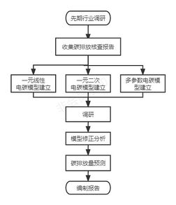
Relying on the technical advantages and experience of the Fujian Metrology Institute in previous carbon emission verification, this paper selects 38 ceramic enterprises in Fujian Province as research objects and establishes enterprise-level electricity-carbon models. By combining multi-source data, we constructed a univariate polynomial linear regression model, a univariate quadratic polynomial linear regression model, and other forms of "multi-data-carbon" models (such as electricity/gas-carbon models). The correlation coefficients of the variables are used to assess the degree of correlation between the independent variable influencing factors and carbon emissions. The technical roadmap is illustrated in Figure 3.1.The enterprise-level electricity-carbon models are validated using the data from the following year. If deviations are found, the reasons are confirmed through multiple methods, such as telephone communication, on-site research, and historical analysis. Corrective parameters are then set for the enterprise-level electricity-carbon models.

4 Content of the study

4.1 Calibration analysis of one-variable polynomial linear regression electricity-carbon model for Fujian ceramics industry

4.1.1 One-variable polynomial linear regression electricity-carbon modeling and corrections

Polynomial regression, a method of regression analysis that examines the polynomials between a dependent variable and one or more independent variables, is called Polynomial Regression. If there is only one independent variable, it is called univariate polynomial regression; if there are more than one independent variables, it is called multivariate polynomial regression [18] , In this study 4.1 uses a univariate polynomial regression equation and 4.2 is a univariate quadratic polynomial regression equation with the formula:

One-variable polynomial regression equations:

${\textstyle y={\beta }_{0}+{\beta }_{1}x+\epsilon }$

(1)

One-variable polynomial regression equations:

${\textstyle y={\beta }_{0}+{\beta }_{1}x+{\beta }_{2}{x}^{2}+}$${\displaystyle \epsilon }$

(2)

where Y is the dependent variable.

X is the independent variable.

${\textstyle {\beta }_{0}}$is the intercept term (the predicted value of Y when X = 0).

${\textstyle {\beta }_{1}}$is the primary term coefficient, which represents the linear effect of X on Y .

${\textstyle {\beta }_{2}}$is the quadratic term coefficient, which represents the effect of X ² on Y .

${\textstyle \epsilon }$ is the error term, representing random fluctuations not captured by the model.

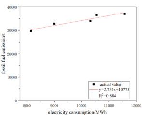
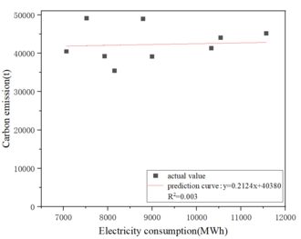
Extract the enterprise's respective corresponding existing historical year to 2020 annual electricity and carbon emissions data, in which the electricity data as the independent variable, carbon emissions data as the dependent variable, to establish a one-dimensional linear electricity and carbon model, and fit the linear curve. Take enterprise 1 as an example, as shown in Figure 4.1.

In accordance with the above method to extract the linear correlation coefficients of the fitted curves of 38 enterprises in turn, it was found that the linear relationship between electricity and carbon emissions of 27 enterprises was poor (the correlation coefficient of the degree of linear fit was less than 0.9), and it was considered that the data of the abnormal years should be excluded and re-modeled, and the linear correlation coefficients of the extracted to the 38 enterprises were as shown in Table 4.1.

company identification	Correlation coefficient (before correction)	Correlation coefficient (corrected)	company identification	Correlation coefficient (before correction)	Correlation coefficient (corrected)
Enterprise 1	0.003	0.9282	Enterprise 20	0.9986	0.9986
Enterprise 2	0.0445	0.7448	Enterprise 21	0.9679	0.9679
Enterprise 3	0.0387	0.6889	Enterprise 22	0.7019	0.9753
Enterprise 4	0.7297	0.9228	Enterprise 23	0.9041	0.9041
Enterprise 5	0.5215	0.8324	Enterprise 24	0.9888	0.9888
Enterprise 6	0.7892	0.9328	Enterprise 25	0.9031	0.9031
Enterprise 7	0.7071	0.9853	Enterprise 26	0.4946	0.9753
Enterprise 8	0.4306	0.9604	Enterprise 27	0.8912	0.9957
Enterprise 9	0.8508	0.9818	Enterprise 28	0.8552	0.9417
Enterprise 10	0.1104	0.8573	Enterprise 29	0.9778	0.9778
Enterprise 11	0.8539	0.8917	Enterprise 30	0.9093	0.998
Enterprise 12	0.9362	0.9362	Enterprise 31	0.5982	0.9185
Enterprise 13	0.1509	0.8729	Enterprise 32	0.3993	0.9091
Enterprise 14	0.1279	0.8348	Enterprise 33	0.4665	0.909
Enterprise 15	0.7107	0.9207	Enterprise 34	0.4304	0.8379
Enterprise 16	0.965	0.9066	Enterprise 35	0.8346	0.938
Enterprise 17	0.5394	0.8607	Enterprise 36	0.752	0.9924
Enterprise 18	0.9377	0.9377	Enterprise 37	0.6411	0.9657
Enterprise 19	0.9314	0.9314	Enterprise 38	0.6567	1.0000

As can be seen from the table, after the model correction, the linear relationship of the electricity-carbon model of the 38 companies is better (the correlation coefficient of the degree of linear fit is greater than 0.9) for 30 companies (78.9%), with the highest value of 1.000 and the lowest value of 0.6889, and the average value reaches 0.9217.

4.1.2 Calibration of one-variable polynomial linear regression electrocarbon models

Selected 30 enterprises with good linear relationship between electricity and carbon emissions and predictable emissions to carry out electricity-carbon model prediction and verification analysis. Based on the verified electricity data for 2021, the electricity-carbon model predicted the emissions in 2021 and compared the deviation with the actual verified carbon emissions. 16 of the 30 ceramic enterprises had a deviation of less than 5% between the predicted and verified emissions; 8 had a deviation of 5%-10%, and 6 had a deviation of more than 10%, as summarized in Table 4.2.

sector

Number of linearly fitting firms

Linear fit case

Number of enterprises with forecast deviations

Forecast deviations

Better linearity Correlation coefficient ≥ 0.9

Poor linearity Correlation coefficient <0.9

Better forecasts Prediction deviation ≤10%

Poor forecasting results Forecast deviation >10%

Mean value of correlation coefficient

Number of enterprises

percentage

Mean value of correlation coefficient

Number of enterprises

percentage

Mean value of forecast deviation

Number of enterprises

percentage

Mean value of forecast deviation

Number of enterprises

percentage

Ceramics

38

0.9518

30

78.9%

0.8246

8

21.1%

30

3.81%

24

80%

19.59%

6

20%

4.2 Calibration analysis of one-quadratic polynomial linear regression electricity-carbon model for Fujian ceramics industry

4.2.1 One-quadratic polynomial linear regression electricity-carbon modeling and corrections

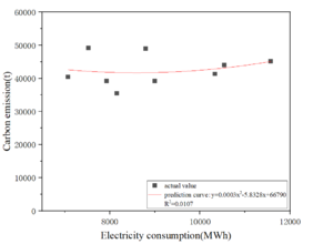
Extract the enterprise's respective corresponding existing historical year to 2020 annual electricity and carbon emissions data, in which the electricity data as the independent variable, carbon emissions data as the dependent variable, the establishment of a one-quadratic polynomial linear regression electricity-carbon model, and fit the linear curve. Take enterprise 1 as an example, as shown in Figure 4.2.

The linear correlation coefficients of the fitted curves of the 38 enterprises were extracted sequentially according to the above method, and it was found that the linear relationship between electricity and carbon emissions of 25 enterprises was poor (the correlation coefficient of the degree of linear fit was less than 0.9), and it was considered that the data of the abnormal years would be excluded and then remodeled, and the linear correlation coefficients of the 38 enterprises were extracted as shown in Table 4.3 (the data of enterprise 2, enterprise 3, enterprise 26, and enterprise 38 were available for 3 years only). years of data, no quadratic fitting was performed).

company identification	Correlation coefficient (before correction)	Correlation coefficient (corrected)	company identification	Correlation coefficient (before correction)	Correlation coefficient (corrected)
Enterprise 1	0.0107	0.9321	Enterprise 20	0.9999	0.9999
Enterprise 2	0.3718	/	Enterprise 21	0.9833	0.9833
Enterprise 3	0.1082	/	Enterprise 22	0.7745	0.9816
Enterprise 4	0.797	0.9237	Enterprise 23	0.9081	0.9081
Enterprise 5	0.6606	0.9011	Enterprise 24	0.9907	0.9907
Enterprise 6	0.7912	0.9643	Enterprise 25	0.9057	0.9057
Enterprise 7	0.9125	0.9864	Enterprise 26	0.4968	/
Enterprise 8	0.456	0.9926	Enterprise 27	0.8922	0.999
Enterprise 9	0.8512	0.9897	Enterprise 28	0.9142	0.997
Enterprise 10	0.2411	0.8858	Enterprise 29	0.9992	0.9992
Enterprise 11	0.8789	0.9937	Enterprise 30	0.9256	0.9997
Enterprise 12	0.9415	0.9415	Enterprise 31	0.6034	0.9418
Enterprise 13	0.1513	0.9999	Enterprise 32	0.7811	0.9258
Enterprise 14	0.128	0.8372	Enterprise 33	0.4715	0.9091
Enterprise 15	0.81	0.952	Enterprise 34	0.6145	0.9101
Enterprise 16	0.993	0.9085	Enterprise 35	0.8685	0.9383
Enterprise 17	0.8613	0.9636	Enterprise 36	0.7693	0.9944
Enterprise 18	0.9507	0.9507	Enterprise 37	0.806	0.9678
Enterprise 19	0.959	0.9259	Enterprise 38	0.7051	/

As can be seen from the table, after the model correction, in addition to four companies that could not be corrected for not quadratic fit, the remaining 34 companies have a better linear relationship (the correlation coefficient of the degree of linear fit is greater than 0.9) of the electricity-carbon model of the 32 companies, which accounted for 94.1%, with the highest value of 0.9999, the lowest value of 0.8372, and the average value reaches 0.9529.

4.4.2 One-quadratic polynomial linear regression electrocarbon model calibration

Selected 32 enterprises with good linear relationship between electricity and carbon emissions can predict the emissions to carry out the electricity-carbon model prediction and verification analysis. Based on the verified electricity data for 2021, the emissions in 2021 were predicted by the electricity-carbon model and compared with the deviation of the actual verified carbon emissions. 9 of the 32 ceramic enterprises had a deviation of less than 5% between the predicted emissions and the verified emissions, 9 had a deviation of 5%-10%, and 14 had a deviation of more than 10%, with an average deviation value of 12.88%, as summarized in Table 4.4.

sector

Number of fitted enterprises

Linear regression fit of a quadratic polynomial in one variable

Number of enterprises with forecast deviations

Forecast deviations

Linear regression with a quadratic polynomial fits better Correlation coefficient ≥ 0.9

Poorly fitted linear regression with a quadratic polynomial Correlation coefficient <0.9

Better forecasts Prediction deviation ≤10%

Poor forecasting results Forecast deviation >10%

Mean value of correlation coefficient

Number of enterprises

percentage

Mean value of correlation coefficient

Number of enterprises

percentage

Mean value of forecast deviation

Number of enterprises

percentage

Mean value of forecast deviation

Number of enterprises

percentage

Ceramics

34

0.9887

32

94.1%

0.8615

2

5.9%

32

4.66%

18

56.3%

23.46%

14

43.7%

4.3 Calibration analysis of linear electricity-carbon model based on carbon emission source decomposition for ceramic industry

4.3.1 Establishment of a linear electricity-carbon model based on carbon source decomposition

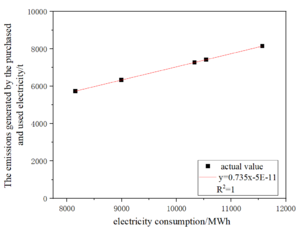
Carbon emission sources in the ceramic industry include: fossil fuel combustion, production process emissions, net purchased use of electricity, and net purchased use of heat. Carbon emissions from each carbon emission source for each historical year of the enterprise and the data of electricity consumption for each historical year are analyzed, taking enterprise 1 as an example, as shown in Figure 4.3.

Figure 4.3-1 The linear relationship between electricity consumption and fossil fuel emission	Figure 4.3-2The linear relationship between electricity consumption and emissions from net purchased electricity

The fitted correlation coefficients of the coupled mapping of electricity and emissions from each source for the 38 enterprises are obtained sequentially as in Table 4.5.

company identification	Electricity emissions from net purchased use	Fossil fuel combustion emissions	Production process emissions	Total emissions	company identification	Electricity emissions from net purchased use	Fossil fuel combustion emissions	Production process emissions	Total emissions
Enterprise 1	1	0.884	/	0.9282	Enterprise 20	1	0.998	/	0.9986
Enterprise 2	1	0.2391	/	0.7448	Enterprise 21	1	0.9553	/	0.9679
Enterprise 3	1	0.5628	/	0.6889	Enterprise 22	1	0.9551	/	0.9753
Enterprise 4	1	0.8382	0.7393	0.9228	Enterprise 23	1	0.9015	0.0124	0.9041
Enterprise 5	1	0.8384	0.9502	0.8324	Enterprise 24	1	0.9631	/	0.99
Enterprise 6	1	0.9466	0.9101	0.9328	Enterprise 25	1	0.8159	0.1325	0.9031
Enterprise 7	1	0.6691	/	0.9853	Enterprise 26	1	0.887	/	0.9753
Enterprise 8	1	0.9516	/	0.9604	Enterprise 27	1	0.5111	/	0.9957
Enterprise 9	1	0.9878	/	0.9818	Enterprise 28	1	0.9012	0.0586	0.9417
Enterprise 10	1	0.8321	/	0.8573	Enterprise 29	1	0.8287	0.6362	0.9778
Enterprise 11	1	0.8592	/	0.993	Enterprise 30	1	0.9967	/	0.998
Enterprise 12	1	0.9329	0.1538	0.9362	Enterprise 31	1	0.8753	/	0.9185
Enterprise 13	1	0.8318	0.7098	0.8729	Enterprise 32	1	0.1744	/	0.9091
Enterprise 14	1	0.9498	0.8424	0.8348	Enterprise 33	1	0.402	/	0.909
Enterprise 15	1	0.6404	/	0.9207	Enterprise 34	1	0.5565	/	0.8379
Enterprise 16	1	0.9743	/	0.9066	Enterprise 35	1	0.9026	/	0.938
Enterprise 17	1	0.7839	/	0.8607	Enterprise 36	1	0.9883	/	0.9924
Enterprise 18	1	0.9039	/	0.9377	Enterprise 37	1	0.9401	/	0.9657
Enterprise 19	1	0.9387	/	0.9055	Enterprise 38	1	0.7138	/	0.9443

By analyzing the correlation coefficients of the coupled mapping fit between electricity and emissions of each emission source, it can be found that if the correlation coefficients of the coupled mapping fit between electricity and emissions of each emission source are high, the correlation coefficients of the coupled mapping fit between electricity and total emissions are also high; the correlation coefficients of the coupled mapping fit between electricity and emissions of the emission sources with a large percentage of carbon emissions have a large effect on the results of the coupled mapping fit between electricity and total emissions and the other way around, it is small, and this also This explains that some enterprises will cause the linear fitting effect of electricity and total emissions to deteriorate due to changes in the production status of some emission sources, thus affecting the prediction bias accuracy of the electricity-carbon model.

4.3.2 Calibration of linear electricity-carbon model based on carbon source decomposition

The coefficients of the coupled mapping fitting function of electricity data and carbon emission data are extracted and summed respectively, resulting in the fitting coefficients of the indirect coupled mapping function of electricity and carbon emissions, from which the fitting equations of the linear electricity-carbon model based on the decomposition of carbon emission sources are obtained as shown in Table 4.6.

company identification	Σa	Σb	one-dimensional fitted equation	company identification	Σa	Σb	one-dimensional fitted equation
Enterprise 1	3.0761	10754	y = 3.0761x + 10754	Enterprise 20	4.1572	435.98	y = 4.1572x + 435.98
Enterprise 2	0.7784	28381	y = 0.7784x + 28381	Enterprise 21	4.4156	-1395.9	y = 4.4156x - 1395.9
Enterprise 3	2.9617	21224	y = 2.9617x + 21224	Enterprise 22	2.6376	7956.1	y = 2.6376x + 7956.1
Enterprise 4	2.7109	19661	y = 2.7109x + 19661	Enterprise 23	3.1791	254.39	y = 3.1791x + 254.39
Enterprise 5	6.9937	-56682	y = 6.9937x - 56682	Enterprise 24	1.6091	-275.43	y = 1.6091x - 275.43
Enterprise 6	4.3428	-11954	y = 4.3428x - 11954	Enterprise 25	1.8788	-3242.4	y = 1.8788x - 3242.4
Enterprise 7	7.0392	-13624	y = 7.0392x - 13624	Enterprise 26	0.5512	35460	y = 0.5512x + 35460
Enterprise 8	7.1051	-20265	y = 7.1051x - 20265	Enterprise 27	0.6593	62415	y = 0.6593x + 62415
Enterprise 9	6.9134	-22856	y = 6.9134x - 22856	Enterprise 28	2.7325	7249.6	y = 2.7325x + 7249.6
Enterprise 10	7.6711	-21576	y = 7.6711x - 21576	Enterprise 29	1.8799	-1716.2	y = 1.8799x - 1716.2
Enterprise 11	5.0651	-15964	y = 5.0651x - 15964	Enterprise 30	3.2377	-49.007	y = 3.2377x - 49.007
Enterprise 12	5.368	4001.4	y = 5.368x + 4001.4	Enterprise 31	3.3286	1682.3	y = 3.3286x + 1682.3
Enterprise 13	4.4572	-6283.2	y = 4.4572x - 6283.2	Enterprise 32	0.8232	24770	y = 0.8232x + 24770
Enterprise 14	0.3976	73120	y = 0.3976x + 73120	Enterprise 33	3.1803	3360.7	y = 3.1803x + 3360.7
Enterprise 15	3.4854	5812.8	y = 3.4854x + 5812.8	Enterprise 34	1.3597	13302	y = 1.3597x + 13302
Enterprise 16	3.6071	-14.172	y = 3.6071x - 14.172	Enterprise 35	3.2349	-2101.9	y = 3.2349x - 2101.9
Enterprise 17	2.5361	5347.8	y = 2.5361x + 5347.8	Enterprise 36	3.5902	-1595.2	y = 3.5902x - 1595.2
Enterprise 18	3.4581	-1254.2	y = 3.4581x - 1254.2	Enterprise 37	2.6712	2391	y = 2.6712x + 2391
Enterprise 19	3.1993	467.58	y = 3.1993x + 467.58	Enterprise 38	4.3805	14245	y = 4.3805x + 14245

Through comparison, it is found that the fitting equations of the linear electricity-carbon model based on the decomposition of carbon emission sources are consistent with the one-dimensional linear fitting equations of the direct coupling of electricity-carbon , which is mainly due to the fact that the independent variables of each linear equation based on the decomposition of carbon emission sources are all the data of electricity, and the use of the direct cumulative is in fact to add up the slopes and the intercepts of the individual linear equations correspondingly, and the final obtained fitting equations of the linear electricity-carbon model based on the decomposition of carbon emission sources are consistent with the one-dimensional linear fitting equations of the direct coupling of electricity-carbon . The resulting linear electricity-carbon model based on carbon emission source decomposition is consistent with the one-dimensional linear fitting equation for the direct coupling of electricity-carbon .

4.4 Calibration Analysis of Linear electricity-carbon model Based on Production Correlation Volume for Fujian Ceramics Industry

4.4.1 Linear electricity-carbon modeling of Ceramic Firms Based on Production Linkage Quantities

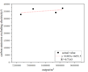
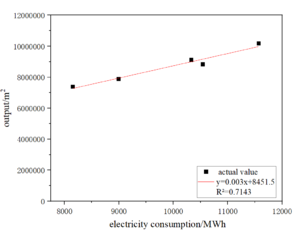
Establish the net purchased electricity generated carbon emissions and electricity data of the fitting relationship equation and deducted from the electricity indirect emissions of other carbon emissions and electricity data of the fitting relationship equation, which in addition to electricity emissions of other carbon emissions and electricity data of the fitting relationship equation through the intermediate amount of data (ceramics production) to establish the relationship between the electricity data and the carbon emissions data, respectively, to obtain the fitting coefficients of the two parts of the fitted model fitting coefficients. The fitting coefficients are added together to obtain the fitting function of the total carbon emissions data and electricity data. Take Enterprise 1 as an example in Figure 4.4.

Figure 4.4-1 The linear relationship between output and carbon emission excluding electricity	Figure 4.4-2 The linear relationship between electricity consumption and output

company identification	Electricity-electricity-carbon emissions correlation coefficient	Electricity - ceramic production correlation coefficient	Correlation coefficient for ceramic production - carbon emissions from de-electricity	company identification	Electricity-electricity-carbon emissions correlation coefficient	Electricity - ceramic production correlation coefficient	Correlation coefficient for ceramic production - carbon emissions from de-electricity
Enterprise 1	1	0.7143	0.95	Enterprise 20	1	0.9925	0.9877
Enterprise 2	1	0.2931	0.4012	Enterprise 21	1	0.9256	0.9151
Enterprise 3	1	0.7996	0.9348	Enterprise 22	1	0.9879	0.9989
Enterprise 4	1	0.8327	0.9673	Enterprise 23	1	0.9783	0.8178
Enterprise 5	1	0.1232	0.1525	Enterprise 24	1	0.6232	0.2041
Enterprise 6	1	0.7041	0.7507	Enterprise 25	1	0.6722	0.5647
Enterprise 7	1	0.7949	0.9319	Enterprise 26	1	0.7241	0.1265
Enterprise 8	1	0.8911	0.8049	Enterprise 27	1	0.9749	0.8616
Enterprise 9	1	0.9332	0.9797	Enterprise 28	1	0.7961	0.9536
Enterprise 10	1	0.9984	0.875	Enterprise 29	1	0.9655	0.9293
Enterprise 11	1	0.9352	0.9595	Enterprise 30	1	0.9862	0.9497
Enterprise 12	1	0.8126	0.6578	Enterprise 31	1	0.0653	0.03152
Enterprise 13	1	0.8392	0.6538	Enterprise 32	1	0.3088	0.6808
Enterprise 14	1	0.0055	0.3605	Enterprise 33	1	0.9757	0.5606
Enterprise 15	1	0.9788	0.6477	Enterprise 34	1	0.86	0.8767
Enterprise 16	1	0.9871	0.9214	Enterprise 35	1	0.9013	0.9411
Enterprise 17	1	0.8661	0.7496	Enterprise 36	1	0.9998	0.986
Enterprise 18	1	0.9489	0.9001	Enterprise 37	1	0.7864	0.717
Enterprise 19	1	0.9525	0.9717	Enterprise 38	1	0.8988	0.8986

As can be seen from the table, the 38 companies based on the amount of production linkage of the coupled mapping fitted a better linear relationship (the correlation coefficient of the degree of linear fit is greater than 0.9) there are 12 companies, accounting for 63.6% of the total number of companies.

company identification	fitting factor		(math.) simultaneous equations	company identification	fitting factor		(math.) simultaneous equations
a	b	a	b
Enterprise 9	6.6717	-19327.1	y=6.6717x- 19327.1	Enterprise 21	4.182456	-241.0406	y=4.182456x- 241.0406
Enterprise 11	5.608158	-17873	y=5.608158x- 17873	Enterprise 22	2.491884	8718.5992	y=2.491884x+ 8718.5992
Enterprise 16	2.82915	8757	y=2.82915x+ 8757	Enterprise 29	1.8495762	-1299.5654	y=1.8495762x-1299.5654
Enterprise 18	3.3891	-1271.357	y=3.3891x- 1271.357	Enterprise 30	4.397316	-14775.8	y=4.397316x- 14775.8
Enterprise 19	3.285485	-338.572	y=3.285485x- 338.572	Enterprise 35	3.186538	-1205.727	y=3.186538x- 1205.727
Enterprise 20	4.110577	565.4129	y=4.110577x+ 565.4129	Enterprise 36	3.720592	-1979.4748	y=3.720592x- 1979.4748

4.4.2 Calibration of Linear Electrocarbon Model for Ceramic Firms Based on Production Correlation Quantities

Based on the annual electricity data of 2021, the emissions in 2021 were predicted by the electricity-carbon model and compared with the deviation of the actual verified carbon emissions. 6 of the 12 ceramic enterprises had a deviation of less than 5% between the predicted emissions and the verified emissions; 3 had a deviation of 5%-10% and 3 had a deviation of more than 10%, with an average value of the deviation of 9.37%.

sector

Number of linearly fitting firms

Linear fit case

Number of enterprises with forecast deviations

Forecast deviations

Better linearity Correlation coefficient ≥ 0.9

Poor linearity Correlation coefficient <0.9

Better forecasts Prediction deviation ≤10%

Poor forecasting results Forecast deviation >10%

Mean value of correlation coefficient

Number of enterprises

percentage

Mean value of correlation coefficient

Number of enterprises

percentage

Mean value of forecast deviation

Number of enterprises

percentage

Mean value of forecast deviation

Number of enterprises

percentage

Ceramics

38

0.9564

12

31.6%

0.682

26

68.4%

12

3.70%

9

75.00%

26.39%

3

25.00%

4.5 Multi-source linear electricity-carbon model calibration analysis for ceramic industry

4.5.1 Establishment and Modification of a Multi-source Linear Electrocarbon Model for Ceramic Firms

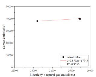
The ceramic enterprises will be corresponding to the existing historical years to 2020 years of electricity and natural gas to calculate carbon emissions, and then with the total emissions to establish "electricity - natural gas - carbon emissions" multi-parameter electricity-carbon model and fit a linear curve, to enterprise 2 as an example of Figure 4.5.

Figure 4.5 The linear fitting curve of the multi-parameter electricity-carbon model of enterprise 2

The correlation coefficients for the degree of linear fit were found to be greater than 0.9 for seven enterprises. The data of abnormal years were considered for re-modeling after elimination, of which enterprise 1 and enterprise 38 could not be corrected due to changes in natural gas consumption over the years, and the remaining 29 enterprises with multi-parameter electricity-carbon models fitted linear curves to obtain the correlation coefficients as shown in the table below.

company identification	Correlation coefficient (before correction)	Correlation coefficient (corrected)	company identification	Correlation coefficient (before correction)	Correlation coefficient (corrected)
Enterprise 1	0.2067	/	Enterprise 20	0.9987	0.9987
Enterprise 2	0.414	0.9555	Enterprise 21	0.9958	0.9958
Enterprise 3	0.3336	0.9927	Enterprise 22	0.9736	0.9268
Enterprise 4	0.3472	0.9714	Enterprise 23	0.8919	0.9963
Enterprise 5	0.6209	0.9955	Enterprise 24	1	1
Enterprise 6	0.149	0.9073	Enterprise 25	0.893	0.9045
Enterprise 7	0.7376	0.9897	Enterprise 26	0.7943	0.9836
Enterprise 8	0.6767	0.9814	Enterprise 27	0.8912	0.9957
Enterprise 9	0.044	0.986	Enterprise 28	0.0683	0.9786
Enterprise 10	0.3339	0.9733	Enterprise 29	0.9121	0.9121
Enterprise 11	0.0946	0.9999	Enterprise 30	0.6901	0.9165
Enterprise 12	0.3745	0.9414	Enterprise 31	0.8529	0.9617
Enterprise 13	0.062	0.9935	Enterprise 32	0.3416	0.9923
Enterprise 14	0.5615	0.7894	Enterprise 33	0.3785	0.9384
Enterprise 15	0.4109	0.9949	Enterprise 34	0.9439	0.9407
Enterprise 16	0.7401	0.9844	Enterprise 35	0.0716	0.9274
Enterprise 17	0.0721	0.9362	Enterprise 36	0.7799	0.9686
Enterprise 18	0.9849	0.9849	Enterprise 37	0.3354	0.9899
Enterprise 19	0.5464	0.9751	Enterprise 38	0.0647	/

As can be seen from the table, except for 2 enterprises that could not be corrected, the rest of the enterprises have been corrected by the model, and the linear relationship of the electricity-carbon model of 36 enterprises is better (the correlation coefficient of the degree of linear fit is greater than 0.9) there are 35 enterprises, which accounts for 97.2% of the total number of enterprises, with the highest value of 1.000, the lowest value of 0.7894, and the average value reaches 0.9633.

4.5.2 Multi-source linear electricity-carbon model calibration for ceramic firms

Thirty-five enterprises with good linear relationship between multi-parameter electric carbon and predictable emissions were selected to carry out electricity-carbon model prediction and verification analysis. Based on the verified electricity data of 2021, the emissions in 2021 were predicted by multi-parameter electric carbon and compared with the deviation of the actual verified carbon emissions. 19 of the 35 ceramic enterprises had a deviation of less than 5% between the predicted emissions and the verified emissions, 8 had a deviation of 5%-10%, and 8 had a deviation of more than 10%, with an average value of deviation of 8.65%.

sector

Number of linearly fitting firms

Multi-parameter linear fitting case

Number of enterprises with forecast deviations

Forecast deviations

Better linear fit Correlation coefficient ≥ 0.9

Poor linear fit Correlation coefficient <0.9

Better forecasts Prediction deviation ≤10%

Poor forecasting results Forecast deviation >10%

Mean value of correlation coefficient

Number of enterprises

percentage

Mean value of correlation coefficient

Number of enterprises

percentage

Mean value of forecast deviation

Number of enterprises

percentage

Mean value of forecast deviation

Number of enterprises

percentage

Ceramics

36

0.9683

35

97.1%

0.7894

1

2.9%

35

3.56%

27

77.1%

25.84%

8

22.9%

V. Conclusion

A horizontal comparison of different electricity-carbon model calibration methods is made. According to the order of testing methods, the calibration of the linear regression electricity-carbon model with a one-variable polynomial is method 1, the calibration of the linear regression electricity-carbon model with a one-variable quadratic polynomial is method 2, the calibration of the electricity-carbon model based on the decomposition of the carbon emission sources is method 3, the calibration of the linear electricity-carbon model based on the production correlation quantity is method 4, and the calibration of the linear electricity-carbon model based on the multi-source data is method 5. The main analyzed data of each calibration method is shown in the table below.

sector	Good linearity of electrocarbon model fit (correlation coefficient ≥ 0.9) Mean value of correlation coefficient					Better forecasts (forecast deviation ≤10%) Mean value of forecast deviation
Method 1	Method 2	Method 3	Method 4	Method 5	Method 1	Method 2	Method 3	Method 4	Method 5
Ceramics	0.9518	0.9587	0.9518	0.9564	0.9683	3.81%	4.66%	3.81%	3.70%	3.56%

Through comparison, it is found that, using the simplest method 1 as the benchmark, the fitted linearity of the electricity-carbon model established by method 2 is not significantly improved, and the prediction deviation is only reduced in the paper-making industry; method 3 is consistent with the essence of method 1, and the results of the fitted linearity and the prediction deviation results are the same as those of method 1, but the method has a certain degree of interpretativeness; method 4 establishes a certain improvement of fitted linearity of the electricity-carbon model compared with method 1; method 5 establishes a certain improvement of the electricity-carbon model fit linearity compared with method 1, and the prediction deviation is reduced. The fitted linearity of the electricity-carbon model established by Method 4 is somewhat improved compared with Method 1; the fitted linearity of the electricity-carbon model established by Method 5 is somewhat improved compared with Method 1, and the prediction deviation is somewhat reduced, which is mainly due to the fact that the method introduces other emission source data, which is conducive to increasing the proportion of the independent variable in the electricity-carbon model, and reducing the impact of power emission fluctuations on linearity. It can be seen that Method 5 is a better solution for the calibration of the electricity-carbon model.

In terms of the difficulty of obtaining data related to carbon emissions, Methods 1 and 2 are the easiest, requiring only electricity and total emissions data; Method 3 is the most difficult, but the calibration results are consistent with Method 1, but Method 3 can be used to analyze and explain the reasons for the poor linearity of the electricity-carbon model and the large prediction bias in some enterprises; Methods 4 and 5, in addition to electricity and total emissions data, need to be combined with the industry's actual situation, to obtain the data of production-related quantities or other emission sources. In addition to electricity and total emissions data, Methods 4 and 5 need to take into account the actual situation of the industry and obtain data on production-related quantities or other emission sources. The difficulty of obtaining data is general, and the production data is more difficult to obtain than the emission source data, because some of the data on production-related quantities (e.g., production output, etc.) may be obtained through statistics or calculations, and internal confidentiality may be involved. The degree of difficulty in obtaining data from each method: Method 1 = Method 2 < Method 5 < Method 4 < Method 3. Meanwhile, for enterprises with large deviations in prediction, through on-site research and comprehensive analysis of historical verification, the main reasons are consistent with the reasons for the poor linear relationship, i.e., first, changes in the production situation, such as a longer period of shutdowns, intermittent production, the addition or subtraction of production lines, and so on; and second, changes in production processes, such as the type or specification of the products produced, such as the type or specification of the products produced. The second is changes in the production process, such as large changes in the types or specifications of the products produced, and changes in energy consumption due to major technological reforms.

Acknowledgements

This work was supported by Sub-project of National Key Research and Development Projects of China(Grant No. 2022YFF0606404)), and Competitive Projects for Public Welfare of Fujian Provincial Department of Science and Technology(Grant No. 2024R1051)).

References

[1] Jindu, Liu Xinping, China's energy structure transition: carbon emission reduction effects, drivers, and carbon peaking exploration, Journal of Safety and Environment (n.d.) 1-8. https://doi.org/10.13637/j.issn.1009-6094.2024.0074.

[2] H. Li, Y. Su, C.J. Ding, G.G. Tian, Z. Wu, Unveiling the green innovation paradox: Exploring the impact of carbon emission reduction on corporate green technology innovation, Technological Forecasting and Social Change 207 (2024) 123562. https://doi.org/10.1016/j.techfore.2024.123562.

[3] X. Xia, X. Zeng, Z. Wang, J. Chen, Y. Cheng, Carbon tax for energy-intensive enterprises: a study on carbon emission reduction strategies, Expert Systems with Applications 257 (2024) 125011. https://doi.org/10.1016/j.eswa.2024.125011.

[4] Z. Zhang, F. Zhang, C. Ma, Does carbon emission trading scheme inhibit corporate executives' pursuit of excess compensation? from a quasi-natural experiment in China, Energy Economics 139 (2024) 107870. https://doi.org/10.1016/j.eneco.2024.107870.

[5] Y. Xia, G. Sun, Y. Wang, Q. Yang, Q. Wang, S. Ba, A novel carbon emission estimation method based on electricity-carbon nexus and non intrusive load monitoring, Applied Energy 360 (2024) 122773. https://doi.org/10.1016/j.apenergy.2024.122773.

[6] D. Wang, J. Gan, J. Mao, F. Chen, L. Yu, Forecasting power demand in China with a CNN-LSTM model including multimodal information, Energy 263 (2023) 126012. https://doi.org/10.1016/j.energy.2022.126012.

[7] Near-Real-Time Carbon Emission Accounting Technology Toward Carbon Neutrality, Engineering 14 (2022) 44-51. https://doi.org/ 10.1016/j.eng.2021.12.019.

[8] H. Chen, S. Wang, J. Li, Y. Yu, D. Li, L. Jin, Y. Guo, X. Cui, A tracking control method for electricity-carbon emission forecasting, Heliyon 10 (2024) e36576. https://doi.org/10.1016/j.heliyon.2024.e36576.

[9] J. Li, C. Zhang, M.R. Davidson, X. Lu, Assessing the synergies of flexibly-operated carbon capture power plants with variable renewable energy in large-scale power systems, Applied Energy 377 (2025) 124459. https://doi.org/10.1016/j.apenergy.2024.124459.

[10] F. Rosner, T. Bhagde, D.S. Slaughter, V. Zorba, J. Stokes-Draut, Techno-economic and carbon dioxide emission assessment of carbon black production, Journal of Cleaner Production 436 (2024) 140224. https://doi.org/10.1016/j.jclepro.2023.140224.

[11] C. Li, N. Shah, Z. Li, P. Liu, Decoupling framework for large-scale energy systems simultaneously addressing carbon emissions and energy flow relationships through sector units: A case study on uncertainty in China's carbon emission targets, Computers & Chemical relationships through sector units: a case study on uncertainty in China's carbon emission targets, Computers & Chemical Engineering 191 (2024) 108840. https://doi.org/10.1016/j.compchemeng.2024.108840.

[12] J. Lotze, M. Moser, G. Savvidis, D. Keles, V. Hagenmeyer, The complementary role of energy system and power grid models: an analysis of the European energy transformation from a holistic perspective, Energy Conversion and Management 315 (2024) 118761. https://doi.org/10.1016/j.enconman.2024. 118761.

[13] Xie Di, Tian Yinglin, Wang Guangqian, Li Tiejian, Zhong Deyu, Research on Carbon Neutral Pathways and Realization Ways in Qinghai Province, Journal of Applied Basic and Engineering Sciences 30 (2022) 1331-1345. https://doi.org/10.16058/j.issn.1005-0930.2022.06.001.

[14] Qigeng Li, Zijin Ji, Hongchao Zhang, Research on the spatio-temporal evolution law of coordinated development of EES in coal mining subsidence area in Shanxi Province, Mining Safety and Environmental Protection (n.d.) 1-7. https://doi.org/10.19835/j.issn.1008-4495.2021.06.023.

[15] Yuheng Ma, Study on the Peak Carbon Emission Pathway in Northeast China in 2030, M.S., Jilin University, 2019. https://kns.cnki.net/kcms2/article/abstract?v=0-LBHIej7QlIw-scoIpCaRgQAwd8uBpjmmWlepxXgKW0bD_ YQf-spfVLcunPm9EgHyLIj4oT82tSVaeVnHo--xkyYiX6lqACkQfPa2Nkn6gjhT0PjKeumdLd_tkRJN5YFulys4gRJc2rAjzjeIFWDDlpYfqvFN1jOVlrC65_ Exu6UR7vEDW3RKMP6XHlH3Ib9u2f11sG6lM=&uniplatform=NZKPT&language=CHS (accessed October 21, 2024).

[16] Chen Maling, State Grid Fujian Xiamen Power Supply Company: "Modularization 2.0" Sponge Substation Completed, China Power Enterprise Management (2024) 96.

[17] Zhoushan, Zhejiang: PV project on grid to help islands achieve "double carbon" goal, Rural Electrification (2021) 59.

[18] B. Lyu, J. Li, Multiple-model polynomial regression and efficient algorithms for data analysis, Theoretical Computer Science 1021 (2024) 114878. https://doi.org/10.1016/j.tcs.2024.114878.