(Tag: Visual edit) |
(Tag: Visual edit) |
||
| Line 78: | Line 78: | ||
{| style="text-align: left; margin:auto;width: 100%;" | {| style="text-align: left; margin:auto;width: 100%;" | ||
|- | |- | ||
| − | | style="text-align: center;" | <math>x'=\ | + | | style="text-align: center;" | <math>x'=\Psi(x,y)-\Omega(x,y),</math> |
|} | |} | ||
|} | |} | ||
| Line 90: | Line 90: | ||
{| style="text-align: left; margin:auto;width: 100%;" | {| style="text-align: left; margin:auto;width: 100%;" | ||
|- | |- | ||
| − | | style="text-align: center;" | <math>\ | + | | style="text-align: center;" | <math>\Psi= \left( \begin{array}{c} \frac{\beta _s IS}{N}+\frac{\beta _a AS}{N}+\frac{\beta _h HS}{N}\\ 0\\ 0\\ 0 \end{array} \right) </math> |
|} | |} | ||
|} | |} | ||
| Line 102: | Line 102: | ||
{| style="text-align: left; margin:auto;width: 100%;" | {| style="text-align: left; margin:auto;width: 100%;" | ||
|- | |- | ||
| − | | style="text-align: center;" | <math>\ | + | | style="text-align: center;" | <math>\Omega= \left( \begin{array}{c} kE\\ -k(1-\sigma )E+(\phi _h+\gamma _s+\delta _s)I\\ -k\sigma E+ \mu A\\ -\phi _h I+(\gamma _h+\delta _h)H \end{array} \right) </math> |
|} | |} | ||
|} | |} | ||
| Line 113: | Line 113: | ||
{| style="text-align: left; margin:auto;width: 100%;" | {| style="text-align: left; margin:auto;width: 100%;" | ||
|- | |- | ||
| − | | style="text-align: center;" | <math>F=\left[\frac{\partial \ | + | | style="text-align: center;" | <math>F=\left[\frac{\partial \Psi_i}{\partial x_j}(E_0)\right]=\left[ \begin{array}{cccc} 0 & \beta _s & \beta _a &\beta _h\\ 0 & 0 & 0 & 0\\ 0 & 0 & 0 & 0\\ 0 & 0 & 0 & 0 \end{array} \right], </math> |
|} | |} | ||
|} | |} | ||
| Line 122: | Line 122: | ||
{| style="text-align: left; margin:auto;width: 100%;" | {| style="text-align: left; margin:auto;width: 100%;" | ||
|- | |- | ||
| − | | style="text-align: center;" | <math>V=\left[\frac{\partial \ | + | | style="text-align: center;" | <math>V=\left[\frac{\partial \Omega_i}{\partial x_j}(E_0)\right]=\left[ \begin{array}{cccc} k & 0 & 0 &0\\ -k(1-\sigma ) &h_1& 0 & 0\\ -k\sigma & 0 & \mu & 0\\ 0 & -\phi _h & 0 & h_2 \end{array} \right] </math> |
|} | |} | ||
|} | |} | ||
| Line 165: | Line 165: | ||
Theorem 1: If <math display="inline">R_0 <1</math> the disease-free equilibrium <math display="inline">E_0</math> is locally asymptotically stable. | Theorem 1: If <math display="inline">R_0 <1</math> the disease-free equilibrium <math display="inline">E_0</math> is locally asymptotically stable. | ||
| − | <span id='theorem-modelo1_simple'></span> | + | <span id='theorem-modelo1_simple'></span>Proof 1: Noting that the two last equations of system ([[#eq-1|1]]) are uncoupled to the remaining equations of the system, we can easily obtain, by direct integration, the following analytical results: |
{| class="formulaSCP" style="width: 100%; text-align: left;" | {| class="formulaSCP" style="width: 100%; text-align: left;" | ||
| Line 181: | Line 181: | ||
In the same way as the total population N is constant, then | In the same way as the total population N is constant, then | ||
| − | <math>S(t)=N-[E(t)-I(t)-A(t)-H(t)-R(t)-F(t)].</math>Thus, the local stability of model ([[#eq-1|1]]) can be studied through the remaining coupled system of state variables, namely, the variables <math display="inline">E</math>, <math display="inline">I</math>, <math display="inline"> | + | <math>S(t)=N-[E(t)-I(t)-A(t)-H(t)-R(t)-F(t)].</math>Thus, the local stability of model ([[#eq-1|1]]) can be studied through the remaining coupled system of state variables, namely, the variables <math display="inline">E</math>, <math display="inline">I</math>, <math display="inline">A</math> and <math display="inline">H</math>. The Jacobian matrix of ([[#eq-1|1]]) restricted to these variables and evaluated at the equilibrium point <math display="inline">E_0=(N,0,0,0,0,0,0)</math> is given by |
{| class="formulaSCP" style="width: 100%; text-align: left;" | {| class="formulaSCP" style="width: 100%; text-align: left;" | ||
| Line 265: | Line 265: | ||
{| style="text-align: left; margin:auto;width: 100%;" | {| style="text-align: left; margin:auto;width: 100%;" | ||
|- | |- | ||
| − | | style="text-align: center;" | <math> | + | | style="text-align: center;" | <math>a_1a_2-a_3 =\left(1-R_ 0\right)\Omega _1+ (1-\sigma ) \Omega _2</math> |
|- | |- | ||
| style="text-align: center;" | <math> + h_ 2 \left(\mu \left(\mu +h_ 2\right)+ k \sigma \left(1+k+\mu +h_ 2\right)\beta _a \right)</math> | | style="text-align: center;" | <math> + h_ 2 \left(\mu \left(\mu +h_ 2\right)+ k \sigma \left(1+k+\mu +h_ 2\right)\beta _a \right)</math> | ||
| Line 283: | Line 283: | ||
<math display="inline">\Omega _2= k \phi \beta _h+k h_ 2 \beta _s +\frac{k^2 \mu \phi \beta _h+k \mu ^2 \phi \beta _h+k \mu \phi h_ 2 \beta _h}{h_ 1 h_ 2}</math>. | <math display="inline">\Omega _2= k \phi \beta _h+k h_ 2 \beta _s +\frac{k^2 \mu \phi \beta _h+k \mu ^2 \phi \beta _h+k \mu \phi h_ 2 \beta _h}{h_ 1 h_ 2}</math>. | ||
| − | <math display="inline">\begin{array}{l}\Omega _3=k \phi \left(k+\mu +2 h_ 2\right)\beta _h\\ +h_1 \left(h_ 2^3+(k+\mu ) h_ 2 \left(\mu +k \sigma \beta _a \right)+2 h_ 2^2 \left(\mu +k\sigma \beta _a \right)+k \phi \beta _h \right)\end{array}</math> | + | <math display="inline">\begin{array}{l}\Omega _3=k \phi \left(k+\mu +2 h_ 2\right)\beta _h\\ +h_1 \left(h_ 2^3+(k+\mu ) h_ 2 \left(\mu +k \sigma \beta _a \right)+2 h_ 2^2 \left(\mu +k\sigma \beta _a \right)+k \phi \beta _h \right).\end{array}</math> |
This shows that Liénard-Chipard's second condition is fulfilled. Therefore, the proof is complete. | This shows that Liénard-Chipard's second condition is fulfilled. Therefore, the proof is complete. | ||
| Line 357: | Line 357: | ||
|} | |} | ||
| − | The estimated basic reproductive number <math display="inline">R_0</math> during the National Period of Healthy Distance, for the epidemic in the CDMX using the SIR model is <math display="inline">R_0=1.21</math>, while for the model ([[#eq-1|1]]) with the parameters of the table [[#table-1|1]] is <math display="inline">R_0=1. | + | The estimated basic reproductive number <math display="inline">R_0</math> during the National Period of Healthy Distance, for the epidemic in the CDMX using the SIR model is <math display="inline">R_0=1.21</math>, while for the model ([[#eq-1|1]]) with the parameters of the table [[#table-1|1]] is <math display="inline">R_0=1.79</math>. On the other hand, the estimated <math display="inline">R_0</math> for the epidemic in Tabasco, that was obtained with the SIR model is <math display="inline">R_0=1.51</math> and the estimation using the model ([[#eq-1|1]]) is <math display="inline">R_0=1.79</math>. This means that the model ([[#eq-1|1]]) predicts that the epidemic will be stronger with respect to the prediction of the SIR model. |
<div id='img-2a'></div> | <div id='img-2a'></div> | ||
| Line 423: | Line 423: | ||
|} | |} | ||
| − | + | Fgures [[#img-5a|5a]] and [[#img-5|5b]] show the estimated cumulative case for Tabasco using the SIR model and the model ([[#eq-1|1]]), respectively. The SIR model estimates around 12,000 total infected cases while the model ([[#eq-1|1]]) estimates around 29000 cumulative infected cases. In September 1st, 2020, the Healthy Secretariat reported 28,471 confirmed infected cases. | |
==6 Numerical results (New Normality Data)== | ==6 Numerical results (New Normality Data)== | ||
| Line 526: | Line 526: | ||
Note that the sensitivity index may depend on several parameters of the system, but also can be constant, independent of any parameter. For example, <math display="inline">Y _\theta ^{R_0}=1</math> means that increasing by a given percentage increases always <math display="inline">R_0</math> by that same percentage. For the mathematical model ([[#eq-1|1]]), the estimation of a sensitive parameter should be carefully done, since a small perturbation in such parameter leads to relevant quantitative changes. On the other hand, the estimation of a parameter with a rather small value for the sensitivity index does not require as much attention to estimate, because a small perturbation in that parameter leads to small changes. | Note that the sensitivity index may depend on several parameters of the system, but also can be constant, independent of any parameter. For example, <math display="inline">Y _\theta ^{R_0}=1</math> means that increasing by a given percentage increases always <math display="inline">R_0</math> by that same percentage. For the mathematical model ([[#eq-1|1]]), the estimation of a sensitive parameter should be carefully done, since a small perturbation in such parameter leads to relevant quantitative changes. On the other hand, the estimation of a parameter with a rather small value for the sensitivity index does not require as much attention to estimate, because a small perturbation in that parameter leads to small changes. | ||
| − | From Table [[#table-2|2]], we see that the most sensitive parameters to the basic reproduction number <math display="inline">R_0</math> of the COVID-19 model ([[#eq-1|1]]) are <math display="inline">\beta _a</math> and <math display="inline">\mu </math>. However, these parameters were chosen from report of Healthy Secretary. In contrast, the lest sensitive parameter is <math display="inline">\ | + | From Table [[#table-2|2]], we see that the most sensitive parameters to the basic reproduction number <math display="inline">R_0</math> of the COVID-19 model ([[#eq-1|1]]) are <math display="inline">\beta _a</math> and <math display="inline">\mu </math>. However, these parameters were chosen from report of Healthy Secretary. In contrast, the lest sensitive parameter is <math display="inline">\delta _h</math>. |
==8 Conclusion== | ==8 Conclusion== | ||
| Line 532: | Line 532: | ||
We have introduced a compartmental mathematical model to understand the dynamic of the COVID 19 pandemic. This model considers a constant population splitted into susceptible class <math display="inline">S</math>, exposed class <math display="inline">E</math>, infectious with symptoms class <math display="inline">I</math>, asymptomatic infectious class <math display="inline">I_a</math>, hospitalized class <math display="inline">H</math>, recovery class <math display="inline">R</math>, and death class <math display="inline">F</math>. The used data correspond to two entities: Mexico city and the State of Tabasco, both considered during the pandemic as “red spotlights”. First of all we showed the existence and stability of the free illnes equilibrium and then we considedered two stages for the numerical study of model: The National Healthy Distance period and the "New normality" period. For comparison reasons, our simulations were done using our model an the classical SIR model. It must be mentioned that for all the numerical simulations, most of the parameters were taken from official government data such as the CONACYT and the updated reference literature linked to the presented models up to 2020. | We have introduced a compartmental mathematical model to understand the dynamic of the COVID 19 pandemic. This model considers a constant population splitted into susceptible class <math display="inline">S</math>, exposed class <math display="inline">E</math>, infectious with symptoms class <math display="inline">I</math>, asymptomatic infectious class <math display="inline">I_a</math>, hospitalized class <math display="inline">H</math>, recovery class <math display="inline">R</math>, and death class <math display="inline">F</math>. The used data correspond to two entities: Mexico city and the State of Tabasco, both considered during the pandemic as “red spotlights”. First of all we showed the existence and stability of the free illnes equilibrium and then we considedered two stages for the numerical study of model: The National Healthy Distance period and the "New normality" period. For comparison reasons, our simulations were done using our model an the classical SIR model. It must be mentioned that for all the numerical simulations, most of the parameters were taken from official government data such as the CONACYT and the updated reference literature linked to the presented models up to 2020. | ||
| − | As a first stage, the study is done during the lockdown (National Healthy Distance) strategy implemented from March 20th to May 31st. For both models, ours and SIR, the obtained numerical estimations fit in an excellent way the reported data, as the accumulated number of infectious disease and the daily infectious cases as well as for the daily deaths (see Figures [[#img-4a|4a]]-[[#img-5|5]]). However, it can be noticed that our model predicts better the infected accumulated cases, the accumulated deaths and the duration of the pandemic (see Figures [[#img-5|5]] and [[#img-8|8]]). With respect to the reproductive number, for the model ([[#eq-1|1]]) and using data and parameters for the CDMX we obtain <math display="inline">R_0=1. | + | As a first stage, the study is done during the lockdown (National Healthy Distance) strategy implemented from March 20th to May 31st. For both models, ours and SIR, the obtained numerical estimations fit in an excellent way the reported data, as the accumulated number of infectious disease and the daily infectious cases as well as for the daily deaths (see Figures [[#img-4a|4a]]-[[#img-5|5]]). However, it can be noticed that our model predicts better the infected accumulated cases, the accumulated deaths and the duration of the pandemic (see Figures [[#img-5|5]] and [[#img-8|8]]). With respect to the reproductive number, for the model ([[#eq-1|1]]) and using data and parameters for the CDMX we obtain <math display="inline">R_0=1.79</math>, while for the SIR model the value is <math display="inline">R_0=1.21</math>. This means that our model is more realistic with respect to pandemic transmision speed, which can be corroborated with the monthly data until May 31, 2020. |
In a second stage, simulations were done using the updated data until August 22th 2020, corresponding to the “New Normality” period when the Mexican government open the activities in sectors which they considered important for the economy, but when the peak's pandemic was not reached yet. The obtained numerical results with the model ([[#eq-1|1]]) fit in a satisfactory way and the predictions improve with respect to the obtained with the classic SIR Model (see Figure [[#img-6|6]]-[[#img-8|8]]). | In a second stage, simulations were done using the updated data until August 22th 2020, corresponding to the “New Normality” period when the Mexican government open the activities in sectors which they considered important for the economy, but when the peak's pandemic was not reached yet. The obtained numerical results with the model ([[#eq-1|1]]) fit in a satisfactory way and the predictions improve with respect to the obtained with the classic SIR Model (see Figure [[#img-6|6]]-[[#img-8|8]]). | ||
| Line 541: | Line 541: | ||
<div id="cite-1"></div> | <div id="cite-1"></div> | ||
| − | '''[[#citeF-1|[1]]]''' B. Tang and X Wang and Q. Li and NL. Bragazzi and S. Tang and Y. Xiao and J. Wu. (2020) "Estimation of the transmission risk of the 2019-ncov and its implication for public health interventions.", Volume 9(2). Journal of Clinical Medicine 462–532 | + | '''[[#citeF-1|[1]]]''' B. Tang and X Wang and Q. Li and NL. Bragazzi and S. Tang and Y. Xiao and J. Wu. (2020) "Estimation of the transmission risk of the 2019-ncov and its implication for public health interventions.", Volume 9(2). Journal of Clinical Medicine 462–532. |
<div id="cite-2"></div> | <div id="cite-2"></div> | ||
| − | '''[[#citeF-2|[2]]]'''. (2020) "Wuhan seafood market pneumonia virus isolate Wuhan-Hu-1". Complete genome 462–532 | + | '''[[#citeF-2|[2]]]'''. (2020) "Wuhan seafood market pneumonia virus isolate Wuhan-Hu-1". Complete genome 462–532. |
<div id="cite-3"></div> | <div id="cite-3"></div> | ||
| − | '''[[#citeF-3|[3]]]''' L.S. Hung. (2003) "The SARS epidemic in Hong Kong: what lessons have we learned?", Volume 96(8). J R Soc Med 374-378 | + | '''[[#citeF-3|[3]]]''' L.S. Hung. (2003) "The SARS epidemic in Hong Kong: what lessons have we learned?", Volume 96(8). J R Soc Med 374-378. |
<div id="cite-4"></div> | <div id="cite-4"></div> | ||
| − | '''[[#citeF-4|[4]]]''' K. K. To and O. T. Tsang and K. H Chan and T. C. Wu and J. M. Chan and W. S. Leung and T. S. Chik and C. Y. Choi and D. H. Kandamby. (2020) "Consistent detection of 2019 novel coronavirus in saliva", Volume 71(15). Clin Infect Dis Off Publ Infect Dis, Soc Am 841–843 | + | '''[[#citeF-4|[4]]]''' K. K. To and O. T. Tsang and K. H Chan and T. C. Wu and J. M. Chan and W. S. Leung and T. S. Chik and C. Y. Choi and D. H. Kandamby. (2020) "Consistent detection of 2019 novel coronavirus in saliva", Volume 71(15). Clin Infect Dis Off Publ Infect Dis, Soc Am 841–843. |
<div id="cite-5"></div> | <div id="cite-5"></div> | ||
| − | '''[[#citeF-5|[5]]]''' E. Zowalaty and E. Mohamed and J. D. Jarhult. (2020) "From SARS to COVID-19: A previously unknown SARS- related coronavirus (SARS-CoV-2) of pandemic potential infecting humans – Call for a One Health approach", Volume 9. One Health | + | '''[[#citeF-5|[5]]]''' E. Zowalaty and E. Mohamed and J. D. Jarhult. (2020) "From SARS to COVID-19: A previously unknown SARS- related coronavirus (SARS-CoV-2) of pandemic potential infecting humans – Call for a One Health approach", Volume 9. One Health. |
<div id="cite-6"></div> | <div id="cite-6"></div> | ||
| − | '''[[#citeF-6|[6]]]''' J. Djordjevic and C. J. Silva and D. F. R. Torres. (2018) "A stochastic SICA epidemic model for HIV transmission", Volume 84. Applied Mathematics Letters 168-175 | + | '''[[#citeF-6|[6]]]''' J. Djordjevic and C. J. Silva and D. F. R. Torres. (2018) "A stochastic SICA epidemic model for HIV transmission", Volume 84. Applied Mathematics Letters 168-175. |
<div id="cite-7"></div> | <div id="cite-7"></div> | ||
| − | '''[[#citeF-7|[7]]]''' A. Rachah and D. F. M Torres. (2016) "Dynamics and optimal control of Ebola transmission", Volume 10. Math Comput Sci 331-342 | + | '''[[#citeF-7|[7]]]''' A. Rachah and D. F. M Torres. (2016) "Dynamics and optimal control of Ebola transmission", Volume 10. Math Comput Sci 331-342. |
<div id="cite-8"></div> | <div id="cite-8"></div> | ||
| − | '''[[#citeF-8|[8]]]''' F. Brauer and C. Castillo-Chavez and Z. Feng. (2019) "Mathematical models in epidemiology". New York: Springer-Verlag | + | '''[[#citeF-8|[8]]]''' F. Brauer and C. Castillo-Chavez and Z. Feng. (2019) "Mathematical models in epidemiology". New York: Springer-Verlag. |
<div id="cite-9"></div> | <div id="cite-9"></div> | ||
| − | '''[[#citeF-9|[9]]]''' F. Gompertz. (1825) "On the nature of the function expressive of the law of h man mortality, and on a new mode of determining the value of life contingencies. In a letter to Francis Baily, Esq. FRS &c", Volume 115. Philosophical transactions of the Royal Society of London 513-583 | + | '''[[#citeF-9|[9]]]''' F. Gompertz. (1825) "On the nature of the function expressive of the law of h man mortality, and on a new mode of determining the value of life contingencies. In a letter to Francis Baily, Esq. FRS &c", Volume 115. Philosophical transactions of the Royal Society of London 513-583. |
<div id="cite-10"></div> | <div id="cite-10"></div> | ||
| − | '''[[#citeF-10|[10]]]''' P.F. Verhulst. (1838) "Notice sur la loi que la population poursuit dans son accroisse- ment. Corresp", Volume 10. Math Phys 113–121 | + | '''[[#citeF-10|[10]]]''' P.F. Verhulst. (1838) "Notice sur la loi que la population poursuit dans son accroisse- ment. Corresp", Volume 10. Math Phys 113–121. |
<div id="cite-11"></div> | <div id="cite-11"></div> | ||
| − | '''[[#citeF-11|[11]]]''' O. Torrealba-Rodríguez and R. A. Conde-Gutiérrez and A. L. Hernández-Javier. (2020) "Modeling and prediction of COVID-19 in Mexico applying mathematical and computational models", Volume 138. Chaos, Solitons and Fractals 109946 | + | '''[[#citeF-11|[11]]]''' O. Torrealba-Rodríguez and R. A. Conde-Gutiérrez and A. L. Hernández-Javier. (2020) "Modeling and prediction of COVID-19 in Mexico applying mathematical and computational models", Volume 138. Chaos, Solitons and Fractals 109946. |
<div id="cite-12"></div> | <div id="cite-12"></div> | ||
| − | '''[[#citeF-12|[12]]]''' F. Ndaïrou and I. Area and J. J. Nieto and D. F. M. Torres "Mathematical modeling of COVID-19 transmission dynamics with a case study of Wuhan". Chaos, Solitons and Fractals 109846 | + | '''[[#citeF-12|[12]]]''' F. Ndaïrou and I. Area and J. J. Nieto and D. F. M. Torres "Mathematical modeling of COVID-19 transmission dynamics with a case study of Wuhan". Chaos, Solitons and Fractals 109846. |
<div id="cite-13"></div> | <div id="cite-13"></div> | ||
| − | '''[[#citeF-13|[13]]]''' A. G. M. Neves and G. Guerrero. (2020) "Predicting the evolution of the COVID-19 epidemic with the A-SIR model: Lombardy, Italy and So Paulo state,Brazi", Volume 413. Nonlinear Phenomena Physica D 132693 | + | '''[[#citeF-13|[13]]]''' A. G. M. Neves and G. Guerrero. (2020) "Predicting the evolution of the COVID-19 epidemic with the A-SIR model: Lombardy, Italy and So Paulo state,Brazi", Volume 413. Nonlinear Phenomena Physica D 132693. |
<div id="cite-14"></div> | <div id="cite-14"></div> | ||
| − | '''[[#citeF-14|[14]]]''' P. Van den Driessche and J. Watmough. (2002) "Reproduction numbers and sub-threshold endemic equilibria for compartmental models of disease transmission", Volume 180. Math Biosci 29–48 | + | '''[[#citeF-14|[14]]]''' P. Van den Driessche and J. Watmough. (2002) "Reproduction numbers and sub-threshold endemic equilibria for compartmental models of disease transmission", Volume 180. Math Biosci 29–48. |
<div id="cite-15"></div> | <div id="cite-15"></div> | ||
| − | '''[[#citeF-15|[15]]]''' A. Liénart and H. Chipart. (1914) "Sur le signe de la partie réelle des racines d'une équation algébrique", Volume 10. J Math Pures Appl (6 éme série) 291-346 | + | '''[[#citeF-15|[15]]]''' A. Liénart and H. Chipart. (1914) "Sur le signe de la partie réelle des racines d'une équation algébrique", Volume 10. J Math Pures Appl (6 éme série) 291-346. |
<div id="cite-16"></div> | <div id="cite-16"></div> | ||
| − | '''[[#citeF-16|[16]]]''' Batista, M. (2020) "Estimation of the final size of the COVID-19 epidemic". medRxiv | + | '''[[#citeF-16|[16]]]''' Batista, M. (2020) "Estimation of the final size of the COVID-19 epidemic". medRxiv. |
<div id="cite-17"></div> | <div id="cite-17"></div> | ||
| Line 592: | Line 592: | ||
<div id="cite-18"></div> | <div id="cite-18"></div> | ||
| − | '''[[#citeF-18|[18]]]''' N. M. Ferguson and D. Laydon and G. Nedjati-Gilani and N. Imai and K. Ainslie and M. Baguelin and S. Bhatia and A. Boonyasiri and Z. Cucunuba and G. Cuomo-Dannenburg. (2020) "Impact of non-pharmaceutical interventions (NPIs) to reduce COVID-19 mortality and healthcare demand", Volume. Imperial College COVID-19 Response Team | + | '''[[#citeF-18|[18]]]''' N. M. Ferguson and D. Laydon and G. Nedjati-Gilani and N. Imai and K. Ainslie and M. Baguelin and S. Bhatia and A. Boonyasiri and Z. Cucunuba and G. Cuomo-Dannenburg. (2020) "Impact of non-pharmaceutical interventions (NPIs) to reduce COVID-19 mortality and healthcare demand", Volume. Imperial College COVID-19 Response Team. |
Revision as of 04:18, 18 November 2023
Abstract
The goal of this work is a dynamic and numerical study of a compartmental mathematical model in order to know the evolution of state variables of the pandemic caused by COVID-19 on red spotlights in México. The model include 7 compartments and the results were compared with the classic SIR model, resulting that our predictions adjusted better the official data. A parameter sensitivity analysis is included.
keywords: COVID-19 pandemic; local stability; Equilibrium point; reproductive basic number.
2 Introduction
In December 31, 2019, Wuhan Municipal Health Commission in Hubei Province, China reported a cluster of 27 pneumonia cases with unknown etiology. The outbreak is associated with common exposures in one wholesale seafood and living animals market in Wuhan City including seven serious cases [1]. The starting point for the first symptomatic case was notified on December 2019. By the 7th of January 2020, the Chinese authorities identified as the causative agent of this outbreak a new type of coronavirus from the family coronaviridae that was called later SARS-CoV-2 which genetic sequence was shared by the Chinese authorities on January the 12th [2]. The via of transmission between human beings, it is similar to the one described by other coronaviruses, by secretions of infected people, mainly by having direct contact with breathing droplets up to 5 microns (allowing them to be transmitted over distances closer than 2 meters) and the contaminated hands or fomites with such secretions, followed by the direct contact of mucosa emissions from the mouth, nose or eyes [3]. The virus SARS-CoV-2 has been founded into the nasopharynx excretions too, including the saliva [4]. On March 11 2020 OMS declared COVID-19 as a world pandemic, since then it is considered the main health problem not only by the mortality rate but also by the secondary effects presented on people such as: Psychological illness, economic loss and the negative impact on their daily activities [5]. From March 20th to May 31st The Secretariat of Health Mexico implemented the social distancing, best known as Healthy Distance (quarantine) because of the COVID-19 pandemic, then to avoid a catastrophic impact on the economy's country, on June 1st, a “The New Normality” started and the goverment reported weekly health alert per region symilar to the traffic light sytem, so with colors there was indicated the type of authorized activities in all economic, labor, educational and social spheres. In this context, the mathematical models of the dynamic transmission on infected diseases have taken an unprecedented relevance. They were applied to help the government`s actions against COVID-19. These models play an important role so as to quantify some possible strategies for mitigation and control of infected diseases [6,7]. There are several models for the infected diseases, since the Clasical SIR Model to more complex proposals [8]. The applied mathematical models, such as Gompertz and Logistic [9,10], have been used with some success to predict the number of infected people with COVID-19. Unfortunately these ones predict on right acurately in short time periods and a huge quantity of data is requested for a good sickness estimation, as it is shown on a recent work done by Torrealba Rodriguez et al. [11], for a COVID-19 estimation in México. On his contributions, Denaiuru et al. [12], makes the proposal for a compartmental mathematical model to the spread of COVID-19 disease, by giving special emphasis on the super-spreaders individuals transmissibility. The problem by working with extensive compartmental models, it is the lack of information for most of the parameters. In a recent work, Neves Armando G.M et. al [13] propose a slightly generalized version of the A-SIR model and propose a scheme for fitting the parameter for the model to real data using the time series only of the deceased individuals. The scheme is applied to the concrete cases of Lombardy, Italy and So Paulo state, Brazil, showing different aspects of the epidemic. In both cases they see strong evidence that the adoption of social distancing measures contributed to a lower increase in the number of deceased individuals when compared to the baseline of no reduction in the infection rate.
In this work, we consider a adaptation of the model in [12] by discarding the super-infectious class but considering the asymtomatic class as an infectious vector. Also we have adjusted the parameters of the resulting model to the Mexican country situations. So we present a consistent compartmental model involving to susceptible class , exposed class , infectious with symptoms class , asymptomatic infectious class , Hospitalized class , recovery class , and death class . Then a qualitative analysis of the model is done. We show the basic reproduction number and the local stability of the free disease equilibrium. The model is solved numerically to predict the dynamic's pandemic in two federal entities which were considered “red spotlights” for the COVID-19 : the CDMX and Tabasco State. As in the whole Country, in both the National Health Distance and the “New Normality” were implemented. Finally we present the estimations with the Classic SIR Model in order to be compared with the proposed model predictions.
3 Model formulation
We propose a compartment model that takes into account the hospitalized individuals and died individuals due to the virus infection. Considering that the size of the population is constant, , we subdivide this population into seven classes: suceptibles class , exposed class , infectious and symptomatic class , infectious and asymptomatic class , sick hospitalized class , recovery class and fatality class , We consider that the rate at which susceptible individuals are infected by having contact with the symptomatic class is and the rate at which succeptible individuals are infected by having contact with the asymptomatic class is . On the other hand, the incubation period of the virus is considered to be and that a fraction of exposed individuals do not develop symptoms, while a fraction of individuals who developed symptoms, require hospitalization. The average recovery period of symptomatic individuals, individuals asymptomatic and hospitalized individuals is represented by , and , respectively. Furthermore, we assume that symptomatic individuals and hospitalized individuals die at a rate and respectively. These relationships between the different classes are represented in the diagram of the Figure 1.
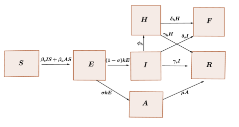
|
| Figure 1: Transference diagram for the proposed COVID-19 model. |
According to the diagram in Figure 1, the dynamics of the epidemic can be represented using the following model of ordinary differential equations
|
|
(1) |
The region of interest for the analysis of the model is
|
|
4 Stability analysis of disease-free equilibrium.
The model (1) has the disease-free equilibrium point . The next generation operator method of Van den Driessche is used to calculate [14]. According to the method, we consider the group of disease variables to and the disease-free variable group to . Thus,
|
|
where
|
|
and
|
|
represent new infections and transitions of individuals between groups, respectively. Therefore
|
|
|
|
and
|
|
where and .
The basic reproduction number, which measures the secondary cases of COVID-19 caused by an infected individual in a susceptible population during your infectious period, is given by , where denotes the spectral radius. That is
|
|
Note that is the sum of three reproductive numbers :
|
|
is given by the product of: the infection rate of susceptible individuals by interaction with symptomatic individuals , the proportion of individuals who develop symptoms and the average duration of an individual in the infectious class . is given by the product of: the infection rate of susceptible individuals by interaction with asymptomatic individuals , the proportion of individuals who do not develop symptoms after the incubation, , and the average duration of an individual in the asymptomatic class Similarly, is given by the product of: the infection rate of susceptible individuals by interaction with hospitalized individuals , the proportion of individuals who develop symptoms and require hospitalization, , and the average duration of an individual to travel from the first contact with the virus to leave the class of hospitalized
Theorem 1: If the disease-free equilibrium is locally asymptotically stable.
Proof 1: Noting that the two last equations of system (1) are uncoupled to the remaining equations of the system, we can easily obtain, by direct integration, the following analytical results:
|
|
(2) |
In the same way as the total population N is constant, then
Thus, the local stability of model (1) can be studied through the remaining coupled system of state variables, namely, the variables , , and . The Jacobian matrix of (1) restricted to these variables and evaluated at the equilibrium point is given by
|
|
The characteristic polynomial of is
|
|
(3) |
where
|
|
(4) |
Using the Liénard-Chipard test [15], all the roots of (the eigenvalues of ) are negative or have negative real part if, and only if, the following conditions are satisfied:
- , .
- .
In order to check these conditions of the Liénard-Chipard test, we rewrite the coefficients , and of the characteristic polynomial in terms of the basic reproduction number :
|
|
(5) |
In this way, the first Liénard-Chipard's condition is evident. On the other hand,
|
|
where
.
.
This shows that Liénard-Chipard's second condition is fulfilled. Therefore, the proof is complete.
5 Numerical results (National Healthy Distance Period)
In this section, we show numerical results for the model (1), using Matlab and Mathematica. To solve SIR model we used the algorithms shown in [16]. The simulations were runed with the official data of the cities of México, CDMX and Tabasco, that was reported by the Healthy Secretariat during the National Healthy Distance Period, from March 20th to May 31st, 2020. The Table 1 shows the parameters used in the numerical simulations. Many of them were obtained from official data from the Mexican government. The infection rate of susceptibles by contact with symptomatic individuals, , was estimated using least squares in the SIR model with reported data.
| Parameter | CDMX | Tabasco | Reference |
| 0.42 | 0.302 | Estimed | |
| 0.39 | 0.42 | Fitting | |
| 0.08 | 0.08 | Fitting | |
| [17] | |||
| 0.68 | 0.68 | [17] | |
| 0.153 | 0.153 | [18] | |
| [17] | |||
| [17] | |||
| [17] | |||
| 0.09 | 0.09 | [17] | |
| 0.035 | 0.035 | [17] |
The estimated basic reproductive number during the National Period of Healthy Distance, for the epidemic in the CDMX using the SIR model is , while for the model (1) with the parameters of the table 1 is . On the other hand, the estimated for the epidemic in Tabasco, that was obtained with the SIR model is and the estimation using the model (1) is . This means that the model (1) predicts that the epidemic will be stronger with respect to the prediction of the SIR model.
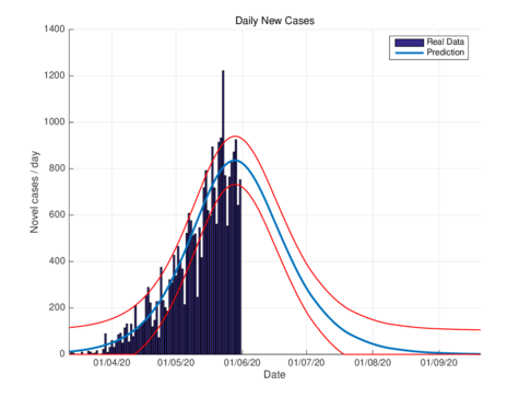
|
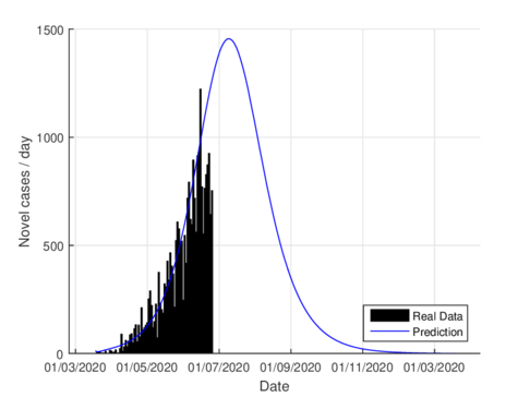
|
| (a) Estimated daily cases for the CDMX, using the SIR model. | (b) Estimated daily cases for CDMX, using the model (1). |
| Figure 2: Daily infectious cases for CDMX. | |
Figures 2a and 2b show the estimations for infections per day using the SIR model and the model (1) for the CDMX. It can be seen that both estimations adjust well the known data. However, with the model (1) the maximum daily infection rate is around 1450 infected, which is reached in mid-June, This is consistent with the reported data. This rate is aproximated better using our nodel instead the SIR model.
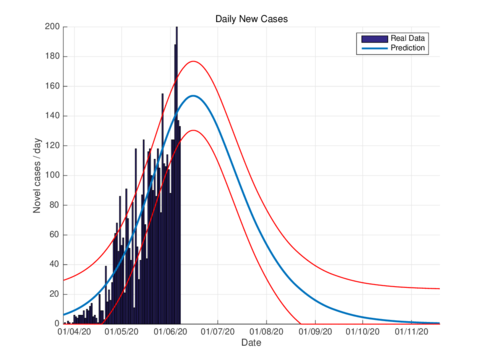
|
|
| (a) Estimated daily new cases for Tabasco using the SIR model. | (b) Estimated daily cases for Tabasco, using the model (1). |
| Figure 3: Daily infectious cases for Tabasco. | |
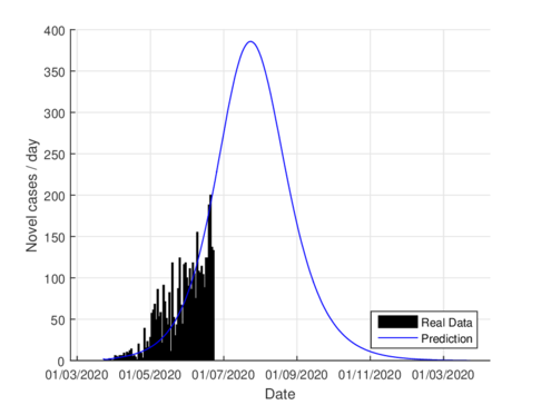
Figures 3a and 3b show the estimates of infections per day using the SIR model and model (1) for Tabasco. Like in the CDMX, the model (1) predicts a maximum of daily cases around 380, that is reached by the end of June 2020, when the confinement was implemented.
|
|
| (a) Estimated cumulative infected cases in CDMX using the SIR model. | (b) Estimated cumulative infected cases in CDMX, using the model (1). |
| Figure 4: Estimated cumulative infected cases for CDMX. | |
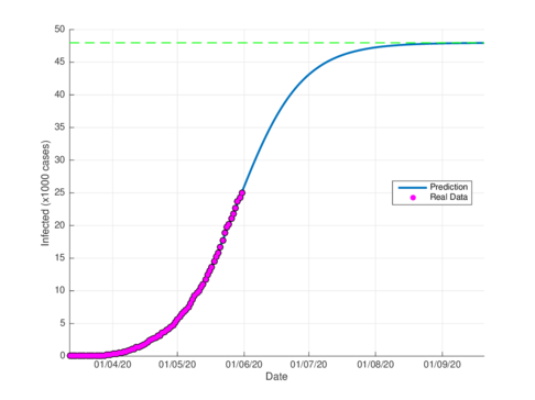
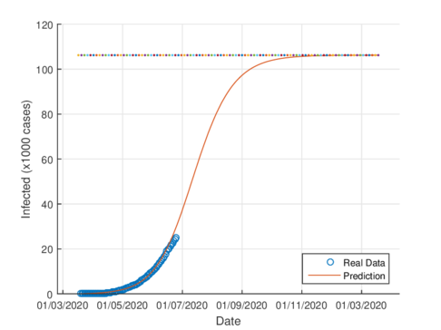
The figures 4a and 4b show the cumulative case estimates for the CDMX, using the SIR model and the model (1), respectively. We can note that, both models adjust appropriately the official data. However, they differ in the total number of people who were infected during the pandemic. The SIR model predicted around 48,000 total cases and the model (1) predicted 105,000 total cases. On the other hand, the Healthy Secretariat reported a total of 99,564 infections at September 1st, 2020.
|
|
| (a) Estimation of cumulative infected cases in Tabasco, using the SIR model. | (b) Estimation of cumulative infected cases in Tabasco, using the model (1). |
| Figure 5: Estimated cumulative infected cases for Tabasco. | |
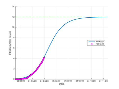
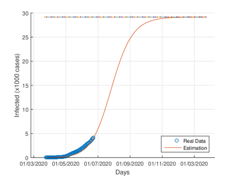
Fgures 5a and 5b show the estimated cumulative case for Tabasco using the SIR model and the model (1), respectively. The SIR model estimates around 12,000 total infected cases while the model (1) estimates around 29000 cumulative infected cases. In September 1st, 2020, the Healthy Secretariat reported 28,471 confirmed infected cases.
6 Numerical results (New Normality Data)
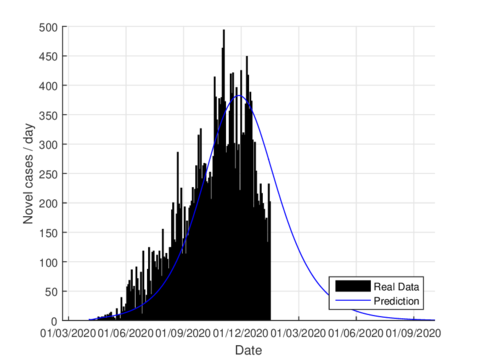
On June 1st, the Mexican government activated the so-called new normality strategy in order to open up activities which are considered essential to reactivate the country's economy. This situation caused a minor increase in almost the entire national territory, furthermore, it caused two plateaus to be observed in the epidemiological curve. If we consider the data on the state of Tabasco after confinement until August 21st, 2020, the parameters were adjusted to this normality and we can see that the model predicts the maximum number of daily cases by mid-July as seen in figure 6. The official reports indicated that the maximum number of daily cases in Tabasco ocurrred in July 12th.
|
| Figure 6: Estimation of daily cases using the model (1) for Tabasco considering the new normality. |
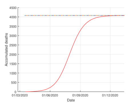
For the case of Tabasco, in the new normality, the model (1) predicts a maximum of 640 hospitalized individuals at the beginning of August and around 4,100 deaths are estimated at the end of the pandemic. In the same way, the model estimates the end of the pandemic by the end of November or the beginning of December as can be seen in Figures 7 and 8 (and 6).
Furthermore, also, we have obtained satisfactory respective estimations for the CDMX, which are not included here to obtain a document not so extensive.
The estimation of indicators such as number of infected, number of hospitalized and deaths are useful for the management of any pandemic, for example, in this case, in the planning of the hospital conversion.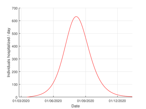
|
| Figure 7: Estimation of hospitalized cases in Tabasco using the model (1). |
|
| Figure 8: Estimated accumulated deaths in Tabasco using the model (1). |
7 Sensitivity analysis of the parameters
In this section we describe the sensitivity analysis of the parameters of model (1), this information is useful to determine the robustness of model predictions to parameter values. Furthermore, it is used to know the parameters that have a high impact on the threshold and these must be handled carefully . More specifically, sensitivity indices allows us to measure the relative change in a variable when a parameter changes. In order to do this analysis, we introduce the following definition.
Definition 1: The normalized forward sensitivity index of , which is differentiable with respect to a given parameter , is defined by
|
|
The values of the sensitivity indices for the parameters values of CDMX and Tabasco, of Table 1, are showed in Table 2. These parameters have been taken from official data. We have seen the mathematical model (1) describes well the real data, giving rise to numerical results showed in the previous section.
| Parameter | CDMX | Tabasco |
Note that the sensitivity index may depend on several parameters of the system, but also can be constant, independent of any parameter. For example, means that increasing by a given percentage increases always by that same percentage. For the mathematical model (1), the estimation of a sensitive parameter should be carefully done, since a small perturbation in such parameter leads to relevant quantitative changes. On the other hand, the estimation of a parameter with a rather small value for the sensitivity index does not require as much attention to estimate, because a small perturbation in that parameter leads to small changes.
From Table 2, we see that the most sensitive parameters to the basic reproduction number of the COVID-19 model (1) are and . However, these parameters were chosen from report of Healthy Secretary. In contrast, the lest sensitive parameter is .
8 Conclusion
We have introduced a compartmental mathematical model to understand the dynamic of the COVID 19 pandemic. This model considers a constant population splitted into susceptible class , exposed class , infectious with symptoms class , asymptomatic infectious class , hospitalized class , recovery class , and death class . The used data correspond to two entities: Mexico city and the State of Tabasco, both considered during the pandemic as “red spotlights”. First of all we showed the existence and stability of the free illnes equilibrium and then we considedered two stages for the numerical study of model: The National Healthy Distance period and the "New normality" period. For comparison reasons, our simulations were done using our model an the classical SIR model. It must be mentioned that for all the numerical simulations, most of the parameters were taken from official government data such as the CONACYT and the updated reference literature linked to the presented models up to 2020.
As a first stage, the study is done during the lockdown (National Healthy Distance) strategy implemented from March 20th to May 31st. For both models, ours and SIR, the obtained numerical estimations fit in an excellent way the reported data, as the accumulated number of infectious disease and the daily infectious cases as well as for the daily deaths (see Figures 4a-5). However, it can be noticed that our model predicts better the infected accumulated cases, the accumulated deaths and the duration of the pandemic (see Figures 5 and 8). With respect to the reproductive number, for the model (1) and using data and parameters for the CDMX we obtain , while for the SIR model the value is . This means that our model is more realistic with respect to pandemic transmision speed, which can be corroborated with the monthly data until May 31, 2020.
In a second stage, simulations were done using the updated data until August 22th 2020, corresponding to the “New Normality” period when the Mexican government open the activities in sectors which they considered important for the economy, but when the peak's pandemic was not reached yet. The obtained numerical results with the model (1) fit in a satisfactory way and the predictions improve with respect to the obtained with the classic SIR Model (see Figure 6-8).
Finally it is important to mention that the inclusion of classes in the population, such as hospitaized and deaths cases, the models provide valuable information to the goverments during the management of pandemics.
BIBLIOGRAPHY
[1] B. Tang and X Wang and Q. Li and NL. Bragazzi and S. Tang and Y. Xiao and J. Wu. (2020) "Estimation of the transmission risk of the 2019-ncov and its implication for public health interventions.", Volume 9(2). Journal of Clinical Medicine 462–532.
[2]. (2020) "Wuhan seafood market pneumonia virus isolate Wuhan-Hu-1". Complete genome 462–532.
[3] L.S. Hung. (2003) "The SARS epidemic in Hong Kong: what lessons have we learned?", Volume 96(8). J R Soc Med 374-378.
[4] K. K. To and O. T. Tsang and K. H Chan and T. C. Wu and J. M. Chan and W. S. Leung and T. S. Chik and C. Y. Choi and D. H. Kandamby. (2020) "Consistent detection of 2019 novel coronavirus in saliva", Volume 71(15). Clin Infect Dis Off Publ Infect Dis, Soc Am 841–843.
[5] E. Zowalaty and E. Mohamed and J. D. Jarhult. (2020) "From SARS to COVID-19: A previously unknown SARS- related coronavirus (SARS-CoV-2) of pandemic potential infecting humans – Call for a One Health approach", Volume 9. One Health.
[6] J. Djordjevic and C. J. Silva and D. F. R. Torres. (2018) "A stochastic SICA epidemic model for HIV transmission", Volume 84. Applied Mathematics Letters 168-175.
[7] A. Rachah and D. F. M Torres. (2016) "Dynamics and optimal control of Ebola transmission", Volume 10. Math Comput Sci 331-342.
[8] F. Brauer and C. Castillo-Chavez and Z. Feng. (2019) "Mathematical models in epidemiology". New York: Springer-Verlag.
[9] F. Gompertz. (1825) "On the nature of the function expressive of the law of h man mortality, and on a new mode of determining the value of life contingencies. In a letter to Francis Baily, Esq. FRS &c", Volume 115. Philosophical transactions of the Royal Society of London 513-583.
[10] P.F. Verhulst. (1838) "Notice sur la loi que la population poursuit dans son accroisse- ment. Corresp", Volume 10. Math Phys 113–121.
[11] O. Torrealba-Rodríguez and R. A. Conde-Gutiérrez and A. L. Hernández-Javier. (2020) "Modeling and prediction of COVID-19 in Mexico applying mathematical and computational models", Volume 138. Chaos, Solitons and Fractals 109946.
[12] F. Ndaïrou and I. Area and J. J. Nieto and D. F. M. Torres "Mathematical modeling of COVID-19 transmission dynamics with a case study of Wuhan". Chaos, Solitons and Fractals 109846.
[13] A. G. M. Neves and G. Guerrero. (2020) "Predicting the evolution of the COVID-19 epidemic with the A-SIR model: Lombardy, Italy and So Paulo state,Brazi", Volume 413. Nonlinear Phenomena Physica D 132693.
[14] P. Van den Driessche and J. Watmough. (2002) "Reproduction numbers and sub-threshold endemic equilibria for compartmental models of disease transmission", Volume 180. Math Biosci 29–48.
[15] A. Liénart and H. Chipart. (1914) "Sur le signe de la partie réelle des racines d'une équation algébrique", Volume 10. J Math Pures Appl (6 éme série) 291-346.
[16] Batista, M. (2020) "Estimation of the final size of the COVID-19 epidemic". medRxiv.
[17]. (2020) "COVID-19, México. https://coronavirus.gob.mx/datos/.". Conahcyt. Mexico.
[18] N. M. Ferguson and D. Laydon and G. Nedjati-Gilani and N. Imai and K. Ainslie and M. Baguelin and S. Bhatia and A. Boonyasiri and Z. Cucunuba and G. Cuomo-Dannenburg. (2020) "Impact of non-pharmaceutical interventions (NPIs) to reduce COVID-19 mortality and healthcare demand", Volume. Imperial College COVID-19 Response Team.
Document information
Published on 13/12/23
Submitted on 18/10/23
Licence: CC BY-NC-SA license
Share this document
claim authorship
Are you one of the authors of this document?