Revision as of 01:02, 13 December 2022

Abstract

Wildfires are an example of a phenomenon that can be investigated using point process theory. We analyze public data from the National Forestry Commission. It consists of wildfire records, specifically their coordinates and dates of occurrence in Mexico State from 2010 to 2018. The spatial component was examined and we found that wildfires tend to cluster. Afterwards, a time series analysis was conducted. This shows that the data comes from a stationary stochastic process. Finally, some spatio-temporal features that demonstrate the point process' regular behavior in space and time were investigated. This research could be a reference to describe wildfire behavior in a specific space and time.

keywords Environmental statistics, point processes, spatio-temporal statistics, wildfires.

1 Introduction

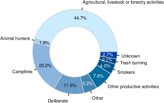
Wildfires are complex phenomena with serious socio-environmental consequences, including economic and biodiversity losses, among others. Anthropogenic factors are responsible for nearly all wildfires in Mexico State, according to data from the National Forestry Commission (Conafor, its Spanish acronym) [1] (see Figure 1).

Figure 1: Mexico State wildfire causes (2010-2018).

There is plenty of specialized literature available on wildfires (see [2] and [3]). The authors of [4] use a logistic regression model to assess the risk of wildfire in Puebla, Mexico, taking into account land cover, meteorological, topographic and social variables. Using two different data sources: Conafor's open data and Modis' (Moderate Resolution Imaging Spectroradiometer) data, the authors of [5] show that wildfire spatial patterns in Mexico tend to cluster. The spatial and temporal relationships between Conafor's wildfire records from 2005 to 2015 and the Standardized Precipitation-Evapotranspiration Index (SPEI) were investigated [6]. Machine learning techniques were used to determine the wildfire propensity in Mexico using Conafor's open data [7].

The spatio-temporal behavior of wildfires could be critical for improving fire management strategies. The point processes approach can be used to model random events in time, space, or space-time, such as wildfires. In this study, we used point processes theory to describe the spatio-temporal behavior of wildfires in Mexico State from 2010 to 2018.

2 Point processes basic theory

A point process is a random set in which the number of points and their locations are both random [8]. A point process could occur in any completely separable metric space ${\textstyle {\mathcal {S}}}$, such as ${\textstyle d}$-dimensional Euclidean space ${\textstyle \mathbb {R} ^{d}}$.

Definition 1: The point process ${\textstyle Y}$, with state space ${\textstyle {\mathcal {S}}}$, is a measurable mapping from a probability space ${\textstyle (\Omega ,{\mathcal {F}},\mathbb {P} )}$ to the measure space of the point process' realizations equipped with the counting measure, ${\textstyle \left({\mathcal {Y}}_{\mathcal {S}}^{\#},{\mathcal {B}}\left({\mathcal {Y}}_{\mathcal {S}}^{\#}\right),\mu _{\#}\right)}$. Where ${\textstyle {\mathcal {Y}}_{\mathcal {S}}^{\#}=\left\lbrace \mu _{\#}:{\mathcal {B}}\left({\mathcal {S}}\right)\rightarrow \mathbb {N} \;\mid \;\mu _{\#}(A)<\infty ,A\in {\mathcal {B}}\left({\mathcal {S}}\right)\right\rbrace }$ is the space of all finite counting measures on a ${\textstyle \sigma }$-algebra ${\textstyle {\mathcal {B}}\left({\mathcal {S}}\right)}$ of subsets of ${\textstyle {\mathcal {S}}}$, ${\textstyle {\mathcal {B}}\left({\mathcal {Y}}_{\mathcal {S}}^{\#}\right)}$ is a ${\textstyle \sigma }$-algebra of subsets of the space ${\textstyle {\mathcal {Y}}_{\mathcal {S}}^{\#}}$ and ${\textstyle \mu _{\#}}$ is the counting measure.

The commutative diagram in Figure 2 illustrates the point process definition.

Figure 2: Commutative diagram of point process definition.

The mapping ${\textstyle \varphi _{A}}$ takes measures ${\textstyle \mu _{\#}\in {\mathcal {Y}}_{\mathcal {S}}^{\#}}$ and maps them into ${\textstyle \mu _{\#}(A)}$. As a result, the mapping ${\textstyle \varphi _{A}}$ in terms of the point process ${\textstyle Y}$ is ${\textstyle \varphi _{A}:Y(\omega ,\cdot )\mapsto Y(\omega ,A)}$.

Furthermore, the commutative diagram reveals the equivalences: ${\textstyle Y(\omega ,A)=\varphi _{A}\left(Y(\omega ,\cdot )\right)=Y_{A}(\omega )}$ and ${\textstyle Y_{A}^{-1}(B)=Y^{-1}\left(\varphi _{A}^{-1}(B)\right)}$, for any ${\textstyle B\in {\mathcal {P}}\left(\mathbb {N} \right)}$, where ${\textstyle {\mathcal {P}}\left(\mathbb {N} \right)}$ denotes the power set of ${\textstyle \mathbb {N} }$, so ${\textstyle \left(\mathbb {N} ,{\mathcal {P}}\left(\mathbb {N} \right)\right)}$ is a measurable space, [9], [10].

The following are some fundamental properties of a point process [10]:

1. Is additive, this is

${\displaystyle Y(\omega ,A_{1}\cup A_{2})=Y(\omega ,A_{1})+Y(\omega ,A_{2}),}$

whenever ${\textstyle A_{1}\cap A_{2}=\varnothing }$, ${\textstyle A_{1},A_{2}\subset {\mathcal {S}}}$ and of course

${\displaystyle Y(\omega ,\varnothing )=0.}$

2. Is locally finite

${\displaystyle \mathbb {P} \left(Y(\omega ,A)<\infty \right)=1,}$

for any ${\textstyle A\subset {\mathcal {S}}}$.

3. Is simple

${\displaystyle \mathbb {P} \left(Y(\omega ,\{{\boldsymbol {s}}\})\leq 1\right)=1,}$

for any point ${\textstyle {\boldsymbol {s}}\in {\mathcal {S}}}$.

For simplification, we will write ${\textstyle Y(\omega ,A)=Y(A)}$ in the foregoing. When the point process ${\textstyle Y}$ is observed, we have a point pattern denoted by ${\textstyle {\boldsymbol {Y}}}$.

In order to generate models, some assumptions about a point process must be made. Stationarity and isotropy are the most important assumptions. The former refers to statistical invariance under translations, whereas the latter refers to statistical invariance under rotations [10], [11]. Nonetheless, some research on non-stationary and anisotropic processes has been conducted (see [12] and [13]).

Definition 2: A point process ${\textstyle Y}$ on ${\textstyle {\mathcal {S}}}$ is stationary if, for any fixed ${\textstyle {\boldsymbol {s}}\in {\mathcal {S}}}$, the distribution of the process ${\textstyle Y+{\boldsymbol {s}}}$ is identical to the distribution of ${\textstyle Y}$.

2.1 Poisson process

The general Poisson point process in some space ${\textstyle {\mathcal {S}}}$ can be defined as follows [10], [11].

Definition 3: The Poisson process ${\textstyle Y}$ on ${\textstyle {\mathcal {S}}}$ with intensity measure ${\textstyle \Lambda }$ is a point process such that:

1. For every compact set ${\textstyle A\subset {\mathcal {S}}}$, the random variable ${\textstyle Y(A)\sim \mathrm {Poisson} \left(\Lambda (A)\right)}$.
2. If ${\textstyle A_{1},\ldots ,A_{n}\subset {\mathcal {S}}}$ are disjoint compact sets, then ${\textstyle Y(A_{1}),\ldots ,Y(A_{n})}$ are independent random variables.

Where the intensity measure ${\textstyle \Lambda }$ is defined, for any ${\textstyle A\subset {\mathcal {S}}}$, as ${\textstyle \Lambda (A)=\mathbb {E} \left(Y(A)\right)}$.

If the state space is ${\textstyle {\mathcal {S}}=\mathbb {R} ^{2}\times \mathbb {R} _{+}}$ and the expected value of the point process ${\textstyle Y}$ in ${\textstyle S\times T}$, with ${\textstyle S\subset \mathbb {R} ^{2}}$ and ${\textstyle T\subset \mathbb {R} _{+}}$, can be written as follows:

where ${\textstyle \lambda >0}$ and ${\textstyle \mu _{L}}$ is the Lebesgue measure, then we have the spatio-temporal homogeneous Poisson point process [14].

The simplest stochastic mechanism for generating point patterns is the homogeneous Poisson point process. As a data model, it is almost never plausible. Regardless, it is the fundamental reference or benchmark model of a point process [8].

The homogeneous Poisson point process is also known as complete spatial (or spatio-temporal) randomness. Additionally, the Poisson point process is stationary and isotropic [10].

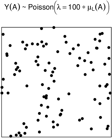
Figure 3 depicts a spatial point pattern generated by a homogeneous Poisson point process.

Figure 3: Simulation of a spatial homogeneous Poisson process.

3 Point pattern's data analysis

Distances between points are a straightforward way to examine a point pattern. The most common statistics used in exploratory analysis of a point pattern are as follows.

3.1 Empty-space function F

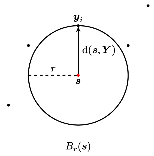
Let ${\textstyle Y}$ be a stationary point process on ${\textstyle {\mathcal {S}}}$. The shortest distance between a given point ${\textstyle {\boldsymbol {s}}\in {\mathcal {S}}}$ and the nearest observed point ${\textstyle {\boldsymbol {y}}_{i}\in {\boldsymbol {Y}}}$ is denoted as ${\textstyle \mathrm {d} ({\boldsymbol {s}},{\boldsymbol {Y}})=\min _{i}\left\lbrace \lVert {\boldsymbol {s}}-{\boldsymbol {y}}_{i}\rVert \right\rbrace }$. It is called the empty-space distance, spherical contact distance, or simply contact distance [8], [10], [11].

Figure 4: Empty-space distance illustration.

Note that

where ${\textstyle B_{r}({\boldsymbol {s}})}$ is the neighborhood of radius ${\textstyle r}$ centered on ${\textstyle {\boldsymbol {s}}}$.

In other words, as shown in Figure 4, the empty-space distance satisfies the logical equivalence of the biconditional (2), ${\textstyle \mathrm {d} ({\boldsymbol {s}},{\boldsymbol {Y}})>r\Leftrightarrow Y\left(B_{r}({\boldsymbol {s}})\right)=0}$.

Moreover, because ${\textstyle \left\lbrace Y\left(B_{r}({\boldsymbol {s}})\right)>0\right\rbrace }$ is measurable, the event ${\textstyle \left\lbrace \mathrm {d} ({\boldsymbol {s}},{\boldsymbol {Y}})\leq r\right\rbrace }$ is measurable, implying that the contact distance is a well-defined random element.

Definition 4: Let ${\textstyle Y}$ be a stationary point process on ${\textstyle {\mathcal {S}}}$. The empty-space function ${\textstyle F}$ is the cumulative distribution function of the empty-space distance

If ${\textstyle Y}$ is a homogeneous Poisson process on ${\textstyle \mathbb {R} ^{d}}$ with intensity ${\textstyle \lambda }$, then the empty-space function is

where ${\textstyle r\geq 0}$, ${\textstyle \mu _{L}\left(B_{1}({\boldsymbol {0}})\right)={\frac {\pi ^{d/2}}{\Gamma \left({\frac {d}{2}}+1\right)}}}$ denotes the volume of the unitary ${\textstyle d}$-ball in ${\textstyle \mathbb {R} ^{d}}$ and ${\textstyle \Gamma }$ is the usual gamma function.

3.2 Nearest-neighbour function G

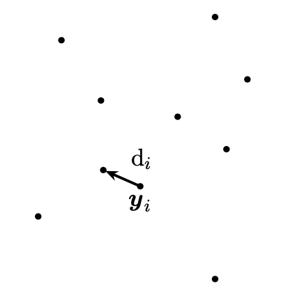
The nearest-neighbour distance, denoted by ${\textstyle \mathrm {d} _{i}=\min _{i\neq j}\left\lbrace \lVert {\boldsymbol {y}}_{i}-{\boldsymbol {y}}_{j}\rVert \right\rbrace }$, is the distance between each point ${\textstyle {\boldsymbol {y}}_{i}\in {\boldsymbol {Y}}}$ and its nearest neighbour in the set ${\textstyle {\boldsymbol {Y}}-\{{\boldsymbol {y}}_{i}\}}$, [8], [10]. It is worth noting that ${\textstyle \mathrm {d} _{i}}$ can also be written as ${\textstyle \mathrm {d} _{i}=\mathrm {d} \left({\boldsymbol {y}}_{i},{\boldsymbol {Y}}-\{{\boldsymbol {y}}_{i}\}\right)}$, [11]. This distance is depicted in Figure 5.

Figure 5: Nearest-neighbour distance illustration.

Definition 5: Let ${\textstyle Y}$ be a stationary point process on ${\textstyle {\mathcal {S}}}$. The nearest-neighbour function ${\textstyle G}$ is the cumulative distribution function of the nearest-neighbour distance

where ${\textstyle r\geq 0}$ and ${\textstyle {\boldsymbol {s}}}$ is any location in the state space ${\textstyle {\mathcal {S}}}$.

If ${\textstyle Y}$ is a homogeneous Poisson process on ${\textstyle \mathbb {R} ^{d}}$ with intensity ${\textstyle \lambda }$, then the nearest-neighbour function is

In this case, we have that ${\textstyle F(r)=G(r)}$, i.e., under complete spatial randomness, the points of the Poisson process are independent of each other, so conditioning does not affect them. Therefore, ${\textstyle F}$ is equivalent to ${\textstyle G}$, [8].

3.3 Intensity

The intensity function describes the first-order properties of a point process [15], [16].

The average number of points per spatial (or spatio-temporal) unit defines the intensity of a point process. In this regard, intensity is analogous to the expected value of a random variable [10].

Similarly, we can investigate the analogue of a point process' variance or covariance throughout the second-order properties.

As we will see in the following, the intensity measure ${\textstyle \Lambda }$ of a point process ${\textstyle Y}$ is clearly a set function, whereas the “instantaneous” intensity function ${\textstyle \lambda }$ is an atomic function.

Definition 6: Let ${\textstyle Y}$ be a point process on ${\textstyle {\mathcal {S}}}$. The first-order intensity is defined as

where ${\textstyle \nu }$ is a suitable measure on ${\textstyle \left({\mathcal {S}},{\mathcal {B}}\left({\mathcal {S}}\right)\right)}$ and ${\textstyle \mathrm {d} {\boldsymbol {s}}}$ defines a infinitesimally small region around ${\textstyle {\boldsymbol {s}}}$.

If ${\textstyle Y}$ is a point process on ${\textstyle \mathbb {R} ^{d}}$ with intensity measure ${\textstyle \Lambda }$, it satisfies

for some function ${\textstyle \lambda }$ and any ${\textstyle A\subset \mathbb {R} ^{d}}$. Then ${\textstyle \lambda }$ is called the intensity function of ${\textstyle Y}$ [10]. If ${\textstyle \lambda }$ is constant, then ${\textstyle Y}$ is said to be homogeneous, otherwise is said to be inhomogeneous [17]. Likewise, if the intensity function exists, we can interpret it as follows:

The ${\textstyle K}$ function and pair correlation are both second-moment properties, so the second-order intensity must be defined [16].

Definition 7: Let ${\textstyle Y}$ be a point process on ${\textstyle {\mathcal {S}}}$. The second-order intensity is defined as

We already have the fundamental elements for defining the following pair of second-order properties.

3.4 K function

The ${\textstyle K}$ function counts the number of locations within a certain radius of a given point (see Figure 6), [11], [18]. Ripley defined it in [19]. We present the following definition [8], [16].

Definition 8: Let ${\textstyle Y}$ be a stationary and isotropic point process on ${\textstyle {\mathcal {S}}}$ with intensity ${\textstyle \lambda }$. The ${\textstyle K}$ function is defined as

where ${\textstyle r\geq 0}$ and ${\textstyle {\boldsymbol {s}}}$ is any location in ${\textstyle {\mathcal {S}}}$.

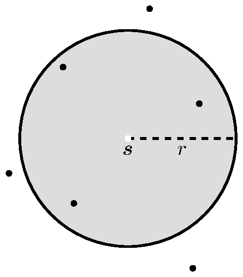
Figure 6: ${\displaystyle K}$ function illustration.

If ${\textstyle {\mathcal {S}}=\mathbb {R} ^{d}}$ and the point process ${\textstyle Y}$ is assumed to be stationary, then hold ${\textstyle \lambda _{2}\left({\boldsymbol {s}},{\boldsymbol {u}}\right)=\lambda _{2}\left({\boldsymbol {s}}-{\boldsymbol {u}}\right)}$. Also, if ${\textstyle Y}$ is isotropic, hence ${\textstyle \lambda _{2}({\boldsymbol {s}}-{\boldsymbol {u}})=\lambda _{2}(r)}$, where ${\textstyle r=\lVert {\boldsymbol {s}}-{\boldsymbol {u}}\rVert }$. These conditions implies that [15], [16],

The above expression provides a relationship between the ${\textstyle K}$ function and the second-order intensity under the assumptions of stationarity and isotropy.

If ${\textstyle Y}$ is a homogeneous Poisson process on ${\textstyle \mathbb {R} ^{d}}$, then the ${\textstyle K}$ function is [10],

3.5 Pair correlation function g

In general, the pair correlation function is a quotient of probabilities; that is, the probability of observing a pair of points separated by a given distance is divided by the same probability, assuming a Poisson point process [8]. In the strictest sense, it is neither a distribution nor a correlation function [16].

Some authors consider the pair correlation function to be the most informative second-order property because it provides information more simply than, say, the ${\textstyle K}$ function [20]. We present the following definition [10], [17].

Definition 9: Let ${\textstyle Y}$ be a point process on ${\textstyle {\mathcal {S}}}$ with intensity function ${\textstyle \lambda }$ and second-moment density ${\textstyle g_{2}}$. The pair correlation function ${\textstyle g}$ is defined as

for any ${\textstyle {\boldsymbol {s}},{\boldsymbol {u}}\in {\boldsymbol {Y}}}$, where the second-moment density is such that

for any compact set ${\textstyle C\subset {\mathcal {S}}\times {\mathcal {S}}}$, where ${\textstyle \nu }$ is a suitable measure on ${\textstyle \left({\mathcal {S}},{\mathcal {B}}\left({\mathcal {S}}\right)\right)}$ (e.g., if ${\textstyle {\mathcal {S}}=\mathbb {R} ^{d}}$, so ${\textstyle \nu =\mu _{L}}$), and ${\textstyle \nu _{[2]}(A_{1}\times A_{2})=\mathbb {E} \left(Y(A_{1})\;Y(A_{2})\right)-\mathbb {E} \left(Y\left(A_{1}\cap A_{2}\right)\right)}$, with ${\textstyle A_{1},A_{2}\subset {\mathcal {S}}}$, is the second factorial moment measure of ${\textstyle Y}$.

If ${\textstyle Y}$ is stationary and isotropic, it follows from (3) that [16], [20],

We can define ${\textstyle g}$ graphically by taking two concentric circles with radius ${\textstyle r}$ and ${\textstyle r+\Delta r}$, where ${\textstyle \Delta r}$ is a small increment, and counting the points that fall within the ring (see Figure 7), [11].

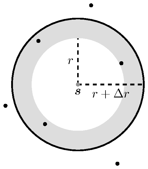
Figure 7: Pair correlation function ${\displaystyle g}$ illustration.

If ${\textstyle Y}$ is stationary and isotropic, the expected number of locations in the ring is ${\textstyle \lambda \;K(r+\Delta r)-\lambda \;K(r)}$. Dividing it by the expected value of points assuming a Poisson process, we obtain

All binomial expansion components in the denominator of the second line in (3.5) lose significance except for ${\textstyle d\;r^{d-1}\Delta r}$, so

Taking the following limit, we get

If ${\textstyle Y}$ is a homogeneous Poisson process on ${\textstyle \mathbb {R} ^{d}}$, then the pair correlation function is ${\textstyle g(r)=1}$.

4 Wildfires' data analysis

Conafor data are licensed for free use (see details in https://datos.gob.mx/libreusomx). It includes wildfire geographical coordinates and dates, as well as variables like forest type affected and severity, among other things.

4.1 Spatial analysis

This spatial analysis focuses on the ${\textstyle F}$ and ${\textstyle G}$ functions to determine whether the wildfire spatial point pattern is aggregated, complete spatial random, or regular. In addition, the intensity was estimated to support the evidence about point pattern behavior.

Plotting the spatial point pattern is a good starting point for understanding its behavior.

Figure 8 shows the spatial point pattern. The wildfires do not appear to be the result of a Poisson process.

There are multiple ways to prove if a point pattern comes from a Poisson point process (see [11]).

Figure 8: Spatial point pattern of Mexico State wildfires.

The simulation envelopes provide a formal way to decide if the spatial pattern comes from the Poisson process. It is equivalent to performing a hypothesis test. The simulation envelopes are obtained under the assumption of a Poisson process [8], [11], [18].

If the empirical curve falls within the envelope, we can conclude that the point pattern comes from a Poisson process.

Figures 9 and 10 show the estimated ${\textstyle F}$ and ${\textstyle G}$ functions, as well as the theoretical functions for the Poisson process and simulation envelopes. For this, we use the R package spatstat [21].

Clearly, the spatial point pattern does not follow the Poisson model.

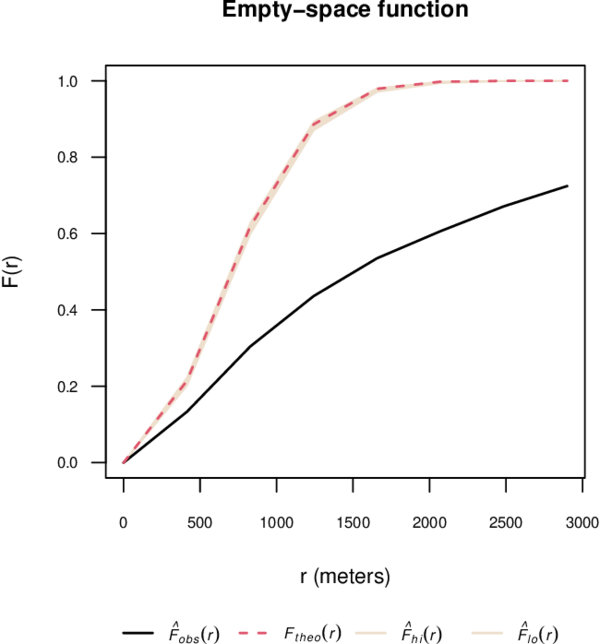
Figure 9: Estimated ${\displaystyle F}$ function and simulation envelopes.

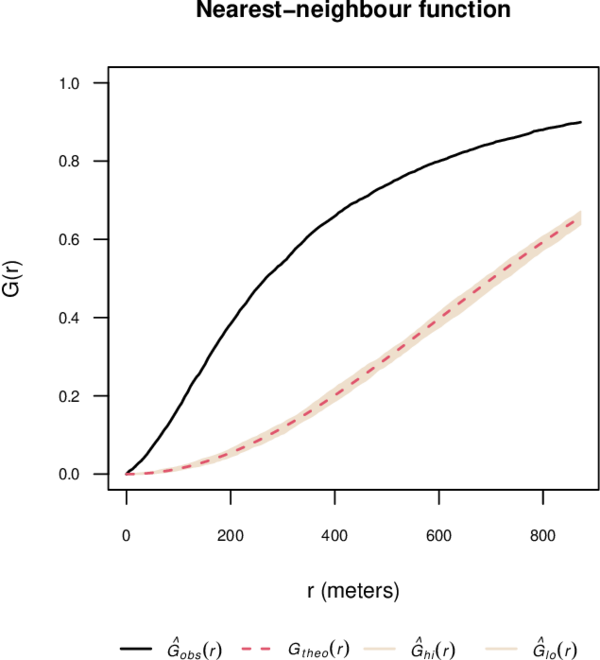
Figure 10: Estimated ${\displaystyle G}$ function and simulation envelopes.

In Figure 9 note that ${\textstyle {\widehat {F}}_{\hbox{obs}}(r)<F_{\hbox{theo}}(r)}$, i.e., the point pattern has longer empty-space distances than a Poisson process. This suggests a clustered point pattern [8]. While in Figure 10 we observe that ${\textstyle {\widehat {G}}_{\hbox{obs}}(r)>G_{\hbox{theo}}(r)}$, i.e., the point pattern has shorter nearest-neighbour distances than a Poisson model, indicating a clustered pattern [8].

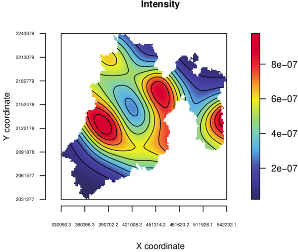
Figure 11 depicts the estimated intensity using a Gaussian kernel with bandwidth of 17 km. It can be used to locate wildfire hotspots.

Figure 11: Estimated intensity.

4.2 Time series analysis

This time series analysis was carried out to describe the temporal behavior of wildfires. Figure 12 displays the daily number of wildfires. This immediately suggests that the wildfire time series is seasonal.

Figure 12: Time series of Mexico State wildfires.

The augmented Dickey-Fuller test is used to prove that the time series is seasonal (see details in [22]). This test is included in the R package tseries [23], where the null hypothesis is that the time series is non-stationary, against the alternative hypothesis that the time series is stationary.

Table 1 displays the results of the augmented Dickey-Fuller test for the wildfire time series, with a significance level of ${\textstyle \alpha =0.05}$.

4.3 Spatio-temporal analysis

To demonstrate clustering or regularity in a spatio-temporal point pattern, the space-time inhomogeneous ${\textstyle K}$ function (STIK) and space-time pair correlation function (STPC) can be used [14].

On the assumption that the point process ${\textstyle Y}$ on ${\textstyle \mathbb {R} ^{d}}$ is second-order stationary, that is, their first-order and second-order properties are invariant under translations, the ${\textstyle K}$ function is [24],

In addition, a spatio-temporal point process is second-order intensity reweighted stationary and isotropic if its intensity function is bounded away from zero, and its ${\textstyle g}$ function is solely determined by ${\textstyle (u,v)}$, where ${\textstyle u=\lVert {\boldsymbol {s}}_{i}-{\boldsymbol {s}}_{j}\rVert }$ and ${\textstyle v=\left|t_{i}-t_{j}\right|}$, with ${\textstyle {\boldsymbol {s}}_{i},{\boldsymbol {s}}_{j}\in \mathbb {R} ^{2}}$, ${\textstyle t_{i},t_{j}\in \mathbb {R} _{+}}$, [14].

Let ${\textstyle Y}$ be a second-order intensity reweighted stationary and isotropic spatio-temporal point process with intensity ${\textstyle \lambda }$; then, from (4), its STIK function is, [14], [24],

where ${\textstyle g(u,v)={\frac {\lambda _{2}(u,v)}{\lambda ({\boldsymbol {s}}_{i},t_{i})\;\lambda ({\boldsymbol {s}}_{j},t_{j})}}}$ is the spatio-temporal pair correlation function ${\textstyle g}$ of ${\textstyle Y}$.

For any inhomogeneous spatio-temporal Poisson process with intensity bounded away from zero,

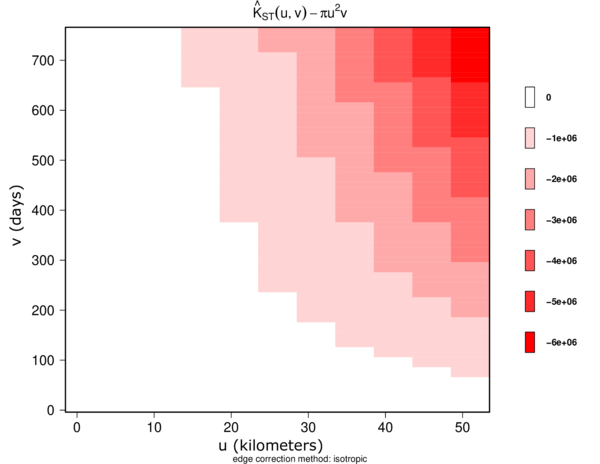
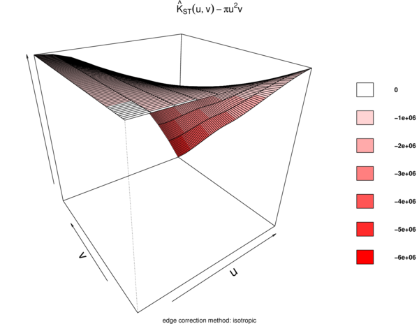
Figures 13 and 14 show the estimated STIK function in contour and perspective plots, respectively.

The values ${\textstyle {\widehat {K}}_{ST}(u,v)-\pi u^{2}v}$ were plotted in order to use them as a measure of spatiotemporal aggregation or regularity. According to [24], ${\textstyle {\widehat {K}}_{ST}(u,v)-\pi u^{2}v<0}$ indicates regularity.

Figure 13: Estimated STIK function contour plot.

Figure 14: Estimated STIK function perspective plot.

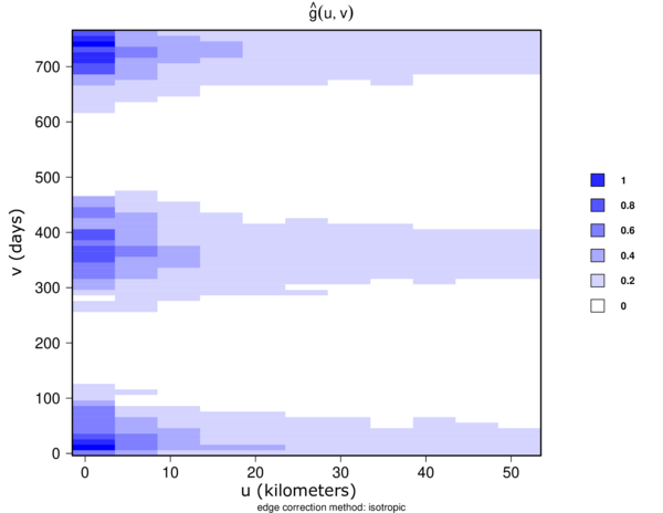
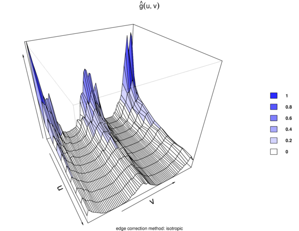
Figures 15 and 16 illustrate estimated STPC function in contour and perspective plots, respectively.

For a spatio-temporal Poisson point process, ${\textstyle g(u,v)=1}$. This reference can be used to determine how much more or less likely it is that a pair of events will occur at specific locations than in a Poisson process of equal intensity [14].

Figure 15: Estimated STPC function contour plot.

Figure 16: Estimated STPC function perspective plot.

Surface behavior is regular; that is, there is yearly seasonality at distances less than 10 km, implying spatio-temporal regularity.

5 Conclusions and perspectives

The spatio-temporal point pattern of Mexico State wildfires from 2010 to 2018 tends to cluster spatially, as shown by Figures 8, 9, 10, and 11.

While the temporal behavior is stationary, as illustrated in Figure 12 and Table 1, there is a yearly wildfire season during the first semester of each year.

Finally, as shown in Figures 13, 14, 15, and 16, we demonstrate that the spatio-temporal behavior is regular. This means that wildfires tend to occur in the same season and in the same areas each year. This regular spatio-temporal behavior suggests that the underlying point process is predictable in some ways.

This research could be expanded by looking into models such as spatio-temporal log-Gaussian Cox processes [25], which can be used to make spatio-temporal predictions.

Acknowledgments

The authors would like to express their gratitude to the Universidad Autónoma Chapingo.

Appendix

This analysis was performed using the statistical programming language R [26]. The developed code is available in the repository:

https://github.com/LuisMunive/Spatio-temporal-point-process-analysis-of-Mexico-State-wildfires.

BIBLIOGRAPHY

[1] Conafor. (2018) "Historical yearly series of wildfires 2010-2018 period" Extracted from: https://datos.gob.mx/busca/dataset/incendios-forestales/resource/5720e224-3d0c-4eed-ac65-ea7aac7d72e8

[2] Rodríguez-Trejo, Dante Arturo. (2014) "Incendios de Vegetación: su ecología, manejo e historia vol. 1", Volume 1

[3] Rodríguez-Trejo, Dante Arturo. (2015) "Incendios de Vegetación: su ecología, manejo e historia vol. 2", Volume 2

[4] Carrillo-García, Rosa Laura and Rodríguez-Trejo, Dante Arturo and Tchikoué, Hubert and Monterroso-Rivas, Alejandro Ismael and Santillan-Pérez, Javier. (2012) "Análisis espacial de peligro de incendios forestales en Puebla, México", Volume 37. Asociación Interciencia. Interciencia 9 678–683

[5] Cisneros-González, Darío and Pérez-Verdín, Gustavo and Pompa-García, Marín and Rodríguez-Trejo, Dante Arturo and Zúñiga-Vásquez, José Manuel. (2017) "Spatial modeling of forest fires in Mexico: an integration of two data sources", Volume 38. Bosque 3 563–574

[6] Pompa-García, Marín and Camarero J., Julio and Rodríguez-Trejo, Dante Arturo and Vega-Nieva, Daniel José. (2018) "Drought and spatiotemporal variability of forest fires across Mexico", Volume 28. Springer Science & Business Media. Chinese Geographical Science 1 25–37

[7] Munive-Hernández, Luis Ramón. (2021) "Predicción espacial de incendios forestales usando aprendizaje máquina"

[8] Baddeley, Adrian and others. (2008) "Analysing spatial point patterns in R", Volume 3. Workshop notes version

[9] Daley, Daryl J and Vere-Jones, David. (2007) "An introduction to the theory of point processes: volume II: general theory and structure". Springer Science & Business Media

[10] Baddeley, Adrian and Bárány, Imre and Schneider, Rolf. (2007) "Spatial point processes and their applications". Springer Science & Business Media. Stochastic Geometry: Lectures Given at the CIME Summer School Held in Martina Franca, Italy, September 13–18, 2004 1–75

[11] Baddeley, Adrian and Rubak, Ege and Turner, Rolf. (2015) "Spatial point patterns: methodology and applications with R". CRC Press

[12] Gabriel, Edith and Rodriguez-Cortes, Francisco and Coville, Jérome and Mateu, Jorge and Chadoeuf, Joël. (2022) "Mapping the intensity function of a non-stationary point process in unobserved areas". Springer Science & Business Media. Stochastic Environmental Research and Risk Assessment 1–17

[13] Villanueva-Morales, Antonio. (2008) "Modified pseudo-likelihood estimation for Markov random fields with Winsorized Poisson conditional distributions". Digital Repository@ Iowa State University, http://lib. dr. iastate. edu/

[14] Gabriel, Edith and Rowlingson, Barry S and Diggle, Peter J. (2013) "stpp: an R package for plotting, simulating and analyzing Spatio-Temporal Point Patterns", Volume 53. Journal of Statistical Software 1–29

[15] Cressie, Noel. (1991) "Statistics for spatial data". John Wiley & Sons

[16] Diggle, Peter J. (2013) "Statistical analysis of spatial and spatio-temporal point patterns". CRC Press

[17] Mller, Jesper and Waagepetersen, Rasmus Plenge. (2003) "Statistical inference and simulation for spatial point processes". Chapman and Hall/CRC

[18] Bivand, Roger S and Pebesma, Edzer J and Gómez-Rubio, Virgilio and Pebesma, Edzer Jan. (2008) "Applied spatial data analysis with R", Volume 747248717. Springer Science & Business Media

[19] Ripley, Brian D. (1977) "Modelling spatial patterns", Volume 39. Wiley Online Library. Journal of the Royal Statistical Society: Series B (Methodological) 2 172–192

[20] Illian, Janine and Penttinen, Antti and Stoyan, Helga and Stoyan, Dietrich. (2008) "Statistical analysis and modelling of spatial point patterns". John Wiley & Sons

[21] Adrian Baddeley and Rolf Turner. (2005) "spatstat: An R Package for Analyzing Spatial Point Patterns", Volume 12. Journal of Statistical Software 6 1–42

[22] Peter J. Brockwell and Richard A. Davis. (2016) "Introduction to Time Series and Forecasting". Springer Science & Business Media. Springer Texts in Statistics

[23] Adrian Trapletti and Kurt Hornik. (2022) "tseries: Time Series Analysis and Computational Finance"

[24] Gabriel, Edith and Diggle, Peter J. (2009) "Second-order analysis of inhomogeneous spatio-temporal point process data", Volume 63. Wiley Online Library. Statistica Neerlandica 1 43–51

[25] Taylor, Benjamin M and Davies, Tilman M and Rowlingson, Barry S and Diggle, Peter J. (2013) "lgcp: an R package for inference with spatial and spatio-temporal log-Gaussian Cox processes", Volume 52. Journal of Statistical Software 1–40

[26] R Core Team. (2022) "R: A Language and Environment for Statistical Computing". R Foundation for Statistical Computing