(Created page with " <div class="center" style="width: auto; margin-left: auto; margin-right: auto;"> L.G. Barbu<sup>ab</sup>, X. Martinez<sup>ab</sup>, S. Oller<sup>ac</sup></div> <div class="...") |
(Tag: Visual edit) |
||
| Line 1: | Line 1: | ||
| − | + | <span id="_GoBack"></span> | |
| − | + | ||
| − | + | ||
| − | + | ||
| − | + | ||
| − | + | ||
| − | <span | + | |
| − | + | ||
| − | + | ||
| − | + | ||
| − | + | ||
| − | + | ||
| − | + | ||
| − | + | ||
| − | + | ||
| − | + | ||
| − | + | ||
| − | + | ||
| − | + | ||
| − | + | ||
| − | + | ||
| − | + | ||
| − | + | ||
| − | + | ||
| − | + | ||
| − | + | ||
| − | + | ||
| − | + | ||
| − | + | ||
| − | + | ||
| − | + | ||
| − | + | ||
| − | + | ||
| − | + | ||
| − | + | ||
| − | + | ||
| − | + | ||
| − | + | ||
| − | + | ||
| − | + | ||
| − | + | ||
| − | + | ||
| − | + | ||
| − | + | ||
| − | + | ||
| − | + | ||
| − | + | ||
| − | + | ||
| − | + | ||
| − | + | ||
| − | + | ||
| − | + | ||
| − | + | ||
| − | + | ||
| − | + | ||
| − | + | ||
| − | + | ||
| − | + | ||
| − | + | ||
| − | + | ||
| − | + | ||
| − | + | ||
| − | + | ||
| − | + | ||
| − | + | ||
| − | + | ||
| − | + | ||
| − | + | ||
| − | + | ||
| − | + | ||
| − | + | ||
| − | + | ||
| − | + | ||
| − | + | ||
| − | + | ||
| − | + | ||
| − | + | ||
| − | + | ||
| − | + | ||
| − | + | ||
==1 Introduction == | ==1 Introduction == | ||
| Line 142: | Line 63: | ||
{| style="text-align: center; margin:auto;" | {| style="text-align: center; margin:auto;" | ||
|- | |- | ||
| − | | <math display="inline">{\mathit{\boldsymbol{\, u}}}_{\mu }\left( {\mathit{\boldsymbol{x}}}_{\mu },t\right) =</math><math>{\epsilon }_{m}\left( {\mathit{\boldsymbol{x}}}_{m},t\right) \cdot \left( {\mathit{\boldsymbol{x}}}_{\mu }-\right. | + | | <math display="inline">{\mathit{\boldsymbol{\, u}}}_{\mu }\left( {\mathit{\boldsymbol{x}}}_{\mu },t\right) =</math><math>{\epsilon }_{m}\left( {\mathit{\boldsymbol{x}}}_{m},t\right) \cdot \left( {\mathit{\boldsymbol{x}}}_{\mu }-\right.\left. {\mathit{\boldsymbol{x}}}_{g}\right) +{\tilde{\mathit{\boldsymbol{u}}}}_{\mu }^{}({\mathit{\boldsymbol{x}}}_{\mu }^{},t) |
| + | </math> | ||
|} | |} | ||
| style="width: 5px;text-align: right;white-space: nowrap;" | (3) | | style="width: 5px;text-align: right;white-space: nowrap;" | (3) | ||
| Line 165: | Line 87: | ||
Moreover, the microscopic position vector <math display="inline">{\mathit{\boldsymbol{x}}}_{\mu }^{}</math> does not appear explicitly in the microstructural strain tensor expression (see Eq. (4)). Consequently, this variable does not appear in the microstructural stress tensor either. Therefore, the periodic microstructure around the macro point <math display="inline">{\mathit{\boldsymbol{x}}}_{m}</math> does not have to be modeled with its exact dimensions. A non-dimensional RVE with the internal distribution and volume fractions of the simple materials is enough to obtain the microscopic strain and stress fields. This is one of the principal advantages of this first-order homogenization approach compared to other multiscale high-order approaches [16]. On the other hand, it can be observed that the kinematically admissible displacement fluctuation option used to satisfy the boundary condition in the RVE problem affects the final macroscopic stress tensor obtained. Several models have been defined that assume different fluctuation fields: | Moreover, the microscopic position vector <math display="inline">{\mathit{\boldsymbol{x}}}_{\mu }^{}</math> does not appear explicitly in the microstructural strain tensor expression (see Eq. (4)). Consequently, this variable does not appear in the microstructural stress tensor either. Therefore, the periodic microstructure around the macro point <math display="inline">{\mathit{\boldsymbol{x}}}_{m}</math> does not have to be modeled with its exact dimensions. A non-dimensional RVE with the internal distribution and volume fractions of the simple materials is enough to obtain the microscopic strain and stress fields. This is one of the principal advantages of this first-order homogenization approach compared to other multiscale high-order approaches [16]. On the other hand, it can be observed that the kinematically admissible displacement fluctuation option used to satisfy the boundary condition in the RVE problem affects the final macroscopic stress tensor obtained. Several models have been defined that assume different fluctuation fields: | ||
| − | • Taylor model (or zero fluctuations): <math display="inline">{\tilde{\mathit{\boldsymbol{u}}}}_{\mu }^{}\left( {\mathit{\boldsymbol{x}}}_{\mu }^{},t\right) = | + | • Taylor model (or zero fluctuations): <math display="inline">{\tilde{\mathit{\boldsymbol{u}}}}_{\mu }^{}\left( {\mathit{\boldsymbol{x}}}_{\mu }^{},t\right) =0\, \forall {\mathit{\boldsymbol{x}}}_{\mu }^{}\in {\Omega }_{\mu }</math> This model gives homogeneous deformation in the microstructural scale level. |
| − | • Linear boundary displacements (or zero boundary fluctuations): <math display="inline">{\tilde{\mathit{\boldsymbol{u}}}}_{\mu }^{}\left( {\mathit{\boldsymbol{x}}}_{\mu }^{},t\right) = | + | • Linear boundary displacements (or zero boundary fluctuations): <math display="inline">{\tilde{\mathit{\boldsymbol{u}}}}_{\mu }^{}\left( {\mathit{\boldsymbol{x}}}_{\mu }^{},t\right) =0\, \forall {\mathit{\boldsymbol{x}}}_{\mu }^{}\in {\partial \Omega }_{\mu }</math>. The deformation of the RVE boundary domain for this class are fully prescribed. |
| − | • Periodic boundary fluctuations: <math display="inline">\, \, {\tilde{\mathit{\boldsymbol{u}}}}_{\mu }^{}\left( {\mathit{\boldsymbol{x}}}_{\mu }^{+},t\right) = | + | • Periodic boundary fluctuations: <math display="inline">\, \, {\tilde{\mathit{\boldsymbol{u}}}}_{\mu }^{}\left( {\mathit{\boldsymbol{x}}}_{\mu }^{+},t\right) =\, {\tilde{\mathit{\boldsymbol{u}}}}_{\mu }^{}\left( {\mathit{\boldsymbol{x}}}_{\mu }^{-},t\right) \, \, \forall \, pair\lbrace {\mathit{\boldsymbol{x}}}_{\mu }^{+},{\mathit{\boldsymbol{x}}}_{\mu }^{-}\rbrace \in {\partial \Omega }_{\mu }</math> . The key kinematical constraint for this class is that the displacement fluctuation must be periodic on the different faces of the RVE. |
• Minimal constraint (or uniform boundary traction): In this constraint the nontrivial solution of <math display="inline">\int_{{\partial \Omega }_{\mu }\, }^{}{\mathit{\boldsymbol{u}}}_{\mu }\, {\otimes }_{s\, }\mathit{\boldsymbol{n}}\, dA</math> is obtained. | • Minimal constraint (or uniform boundary traction): In this constraint the nontrivial solution of <math display="inline">\int_{{\partial \Omega }_{\mu }\, }^{}{\mathit{\boldsymbol{u}}}_{\mu }\, {\otimes }_{s\, }\mathit{\boldsymbol{n}}\, dA</math> is obtained. | ||
Revision as of 20:35, 1 May 2022
1 Introduction
Almost all existing materials around us can be considered heterogeneous structures or composite materials, since they are composed by several phases or components at certain spatial scale of observation. Prediction of the physical and chemical behaviour of such materials is a complicated target. Their properties, also called efective or homogenized properties, fully depend on the internal microstructure which can be different from one to another composite in morphology, volume fraction, and of course, in properties of constituents. The interaction between components, failure of interfaces capacity or damage because of fracture of the constituents must be also considered. Therefore, obtaining a good characterization of composite materials behaviour is in general a complex issue and requires considering suitable and sophisticated methods [1].
1.1 State of the art for composite homogenization techniques
A composite material is defined as a complex structure characterized by two or more components with different mechanical, thermal and/or chemical properties. The combinations of multiple constituents leads to a new material that usually improves significantly the properties of the base materials. Examples of composites are the fiber reinforced polymers (FRP) or even the reinforced concrete used in civil engineering applications. From a numerical point of view the simulation of these non-homogeneous materials has always represented a challenge because of the interaction between the different constituent materials, associated to the usually complex composite internal microstructure. Modelling each single component of the composite, also called Direct Numerical Simulation (DNS), provides the highest level of accuracy but, at the same time, the simulation of large-scale structures implies a prohibitively expensive computational cost. For this reason, to increase the efficiency of the simulations, the non-homogeneous composite materials are often treated as homogeneous continua characterized by more complex constitutive models. The classical mixing theory [2] is one of the most used phenomenological homogenization methods. The mechanical behavior of the composite is obtained as the homogenized results of the mechanical properties of the components assuming an iso-strain compatibility equation among them. Another important formulation, based on a phenomenological homogenization, that accounts for a more general topological distribution of the components in the composite is the Serial/Parallel (SP) mixing theory. This theory, detailed in [3][4], distinguishes two behaviors of the composite depending on the alignment of the fiber on the composite. Isostrain and iso-stress conditions are applied in the fiber direction, and in the orthogonal direction, respectively. The serial-parallel theory obtains the response of the composite assuming certain iso-stress and iso-strain boundary conditions that regularizes the response of the material if it is defined with several laminates. However, phenomenological homogenization describes the behavior of composite materials only at macroscopic level. This method cannot describe accurately the stress and strain distribution among the components. Thanks to the increase in computer capabilities, multiscale homogenizations started to become a viable alternative [5].
In the last decade, several multiscale approaches have been developed becoming nowadays in an essential technique for modelling composites materials. This is because, even today performing a full direct numerical simulation including all the heterogeneities leads to a huge problem, which is expensive and unworkable from a computational cost point of view. On the other hand, carrying out numerous experiments on many material samples with different geometrical and physical properties is practically impossible because of time and cost.
In a general sense, it is possible classify the multiscale models into the concurrent method [6-9] and the homogenization method, on the latter one will be focused this article. The main feature of a generic concurrent multiscale method is that coarse and fine-scale regions are processed simultaneously. The links between different scales are accounted considering displacement compatibility and momentum balance across the whole solid [1].
Therefore, this framework considers a strong coupling between the scales. On the other hand, the multiscale homogenization method is based on the principle of separation of scales and then, micro-scale length is assumed much smaller than macro-scale length [10]. Consequently, in this approach the length scales of micro and macro-problems must be suffciently separate.
Multiscale homogenization method which uses the concept of Representative Volume Element (RVE) [11,12] together with suitable computational approaches has emerged as one of the most promis-ing formulation to address the response of composites structures. The RVE is employed to determine the homogenized properties and behaviour of a material point at the macro-scale level. It is defined as a microstructural subregion and must be large enough to be statistically representative of the composite material including all its microscopic heterogeneities [13-15]. However, it must remain suffciently small to be considered as a volume element of the structure, fulfill space separation condition and also due to computational efficiency [16].
1.2 Eco-composites in the aeronautical field
Fibre reinforced polymers (FRP) have gained in importance in aviation and other transportation sectors due to their excellent mechanical properties combined with relatively low weight. High performance composites like carbon fibre reinforced polymers (CFRP) and also glass fibre reinforced polymers (GFRP) are used in primary and secondary structures of modern aircrafts. They enable the construction of lighter and more efficient aircraft resulting in the reduction of fuel consumption and increased payloads Carbon fibres consume high amounts of energy during the production phase. Therefore it is of high interest to reduce the consumption of synthetic materials in favour of bio-based materials in certain applications. Bio-based (renewable) materials like natural fibres have been under investigation for a long time for their use in composites but they have not been introduced into a modern aircraft in noticeable amounts yet. The lack of experience and confidence in the long-term performance and mechanical properties of composites containing natural fibres is still an obstacle for their usage in safety relevant applications like primary structures (e.g. fuselage). However, secondary structures and interior composites which are not stressed on such high levels offer possible areas of application in aviation [17].
1.3 Current formulation
In the context of solid mechanics and multiscale computational homogenization, one of the most extended and popular method is called First-Order Computational Homogenization (FOCH) [13,18]. In this approach, the macro-scale strain tensor (or deformation gradient tensor) is used as input to solve the micro-scale BVP. The material stress-strain relationship is obtained from the solution of problem at the micro-scale i.e. the RVE which contains the detailed modeling of the internal heterogeneous structure of the composite. Therefore, it does not require any composite constitutive assumption or compatibility equation to address the composite response [19]. Also, there are no restrictions on the constitutive model used in the component materials, even non-linear materials and time-dependency models can be taken into account [20, 21]. A comprehensive description of the formulation can be found in [1] and [5].
2 Numerical homogenization procedure - Classical First-Order Multiscale Method
One of the most popular multiscale methods is the first-order homogenization. In this procedure, the strain obtained when analyzing the macroscopic structure is used to define the boundary conditions, applied on a Representative Volume Element (RVE), to solve the Boundary Value Problem (BVP) at the microscale. The basic principles of homogenization method were provided by Suquet [22] to obtain the constitutive equation for the homogenized properties of a heterogeneous material. The unit cell is defined as a microscopic subregion that is representative of the entire microstructure in an average sense. The RVE is employed to obtain the effective properties for the homogenized material because it is assumed that it must contain a sufficient number of heterogeneities [5], [14]. The solution of the problem at the microscale, under such conditions, acts as an equivalent constitutive law for the macroscale, and it provides material stiffness and stresses as the volume average of the microscopic ones. This equivalent constitutive law is used in all the integration points of the macroscopic model to obtain the global response of the structure. When dealing with nonlinear microstructures, it will lead to an iterative procedure in which the RVE must be solved for different boundary conditions until both scales reach equilibrium, ensuring consistency between the micro- and macroscale solutions. The first-order homogenization technique developed assumes a scale separation between the macro and the microscale. This is, the characteristic length of the microscale should be much smaller than the length of the macroscale elements, [23]. On each integration point of the discretized macroscale domain, the macroscopic strain tensor provides the input variables for the microscale domain. Then, the solution of the microscopic behavior of the RVE provides the macroscopic output and properties of the equivalent homogeneous medium. In this paper, for the sake of simplicity, the procedure assumes small displacements and a quasi-static behavior in both macro and micro scales. However, the methodology proposed can be extended to other cases.
2.1 Macro to micro transition
At the macro level, the starting point for a kinematically based computational homogenization method is the assumption that the mechanical strain tensor, , at each point of the macroscale domain, (where the position is defined through the vector ), and at a certain instant t can be obtained as the volume average of the microscopic mechanical strain field, , defined at each point of the microscale domain, (where the position is defined through the vector ), and at the same instant t as:
|
|
(1) |
From the Eq. (1) the microscopic strain field can be expressed as the symmetric gradient of the microscopic displacement field, :
|
|
(2) |
Without loss of generality, we can decompose the microscale displacement as:
|
|
(3) |
where and are respectively the constant and fluctuation displacements with respect to the average fields (the centroid of the microscale) at each instant t.
In the same way the microscopic strain can be divided in two parts, a constant one from the macroscopic scale ( ) and the contribution of fluctuation ( ).
|
|
(4) |
Moreover, the microscopic position vector does not appear explicitly in the microstructural strain tensor expression (see Eq. (4)). Consequently, this variable does not appear in the microstructural stress tensor either. Therefore, the periodic microstructure around the macro point does not have to be modeled with its exact dimensions. A non-dimensional RVE with the internal distribution and volume fractions of the simple materials is enough to obtain the microscopic strain and stress fields. This is one of the principal advantages of this first-order homogenization approach compared to other multiscale high-order approaches [16]. On the other hand, it can be observed that the kinematically admissible displacement fluctuation option used to satisfy the boundary condition in the RVE problem affects the final macroscopic stress tensor obtained. Several models have been defined that assume different fluctuation fields:
• Taylor model (or zero fluctuations): This model gives homogeneous deformation in the microstructural scale level.
• Linear boundary displacements (or zero boundary fluctuations): . The deformation of the RVE boundary domain for this class are fully prescribed.
• Periodic boundary fluctuations: . The key kinematical constraint for this class is that the displacement fluctuation must be periodic on the different faces of the RVE.
• Minimal constraint (or uniform boundary traction): In this constraint the nontrivial solution of is obtained.
For the displacement fields, we use periodic boundary conditions since they generally provide an intermediate and more exact response compared to other type of boundary conditions, as it is described in [14],[16],[5].
2.2 Micro to macro transition
Following the solution of the BVP [11] we get the homogenized macroscopic stress tensor. In addition, we can obtain the homogenized constitutive tensor. The homogenized macroscopic stress tensor can be obtained as the microscopic stress field of the RVE averaged on the volume as [23]:
|
|
(5) |
2.3 Material homogenized properties
The macroscopic constitutive relation defined by the homogenized properties of the RVE can be obtained after the solution of the microscale BVP. Assuming the equilibrium of the microscale expressed as:
|
|
(6) |
As is described in [15], the homogenized constitutive tensor can be defined as:
|
|
(7) |
where is the material constitutive tensor of the RVE. The evaluation of the homogenized constitutive tensor is performed with a perturbation method, also see [16][21]. For each column j of the constitutive tensor, a small strain perturbation ( ) is applied to the RVE in order to obtain, along with Eq. (6), a perturbed stress tensor ( ). The j columns of the homogenized constitutive tensor can be obtained as:
|
|
(8) |
3 Four point bending nonlinear simulation of eco-composite
The numerical simulations and the experimental results shown in this section have been conducted under the framework of the project ECO-COMPASS, funded by the European Union’s Horizon 2020 research and innovation programme under grant agreement No 690638 and the Ministry for Industry and Information of the People’s Republic of China under grant agreement No [2016]92.
The main objective of the cooperation of the Chinese and European partners is to develop and assess multifunctional and ecologically improved composites from bio-sourced and recycled materials for application in aircraft secondary structures and interior.
In this context, a green honeycomb + plain weave ramie fabric/rosin prepreg (SRR) specimen has been tested experimentally and afterwards analyzed with a multiscale numerical simulation.
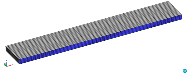
The numerical model used for the analisis of the Sandwich eco-composite is shown in Figure 2. It has 7200 linear hexahedra elements with a total of 9072 nodes. Dimension of the test specimen is 400*75*12 (in millimetres), same as shown in the experimental program conducted by the partners at the University of Manchester (UNIMAN) as shown in Figure 1.
Regarding the composite used for the skin of the sandwich paned, two eco-composite panels (CR and RR) were manufactured at AI-CRT and delivered to UNIMAN for mechanical testing. Prepreg materials for composite manufacturing was prepared and provided by Chinese partners. Details of the prepreg material used with a number, orientation and dimensions of the plies and the thickness for the skin composite are given in table 1. Only the ramie rosin RR composite has been considered for the numerical simulation of the four point bending case so the data for this composite is shown.
| Materials | AGMP 3600 rosin based
epoxy resin /plain ramie fibre fabric prepreg |
| Prepreg fibre volume (%) | 51.4 |
| Number of layers | 10 |
| Orientation | 0° warp |
| Dimensions (mm) | 500*600 |
| Number of parts cured | 1 |
| Measurred thickness (mm) | 2.11 ± 0.01 |
The ramie rosin sandwich (SRR) composite has a core made from 1 layer of green honeycomb oriented in the L direction and the skins are made from the woven composite described in Table 1, applied in 5 layers in the 0º warp direction. The total thickness of the panel is 12 mm.
In order to perform a multiscale analysis of the SRR sandwich panel two different micromodels have been developed. The first one is representatitve of the woven skin composite and will be described in section 3.1. For the core of the sandwich specimen a honeycomb representative volume has been developed that will be described in section 3.2.
The boundary conditions considered in the numerical simulation are consistent with the experimental setup. In Figure 3 the position of the applied loads and of the restraints is indicated, as specified by the AITM 1-0018.
3.1 Representative volume element of woven ramie fibres in an epoxy matrix
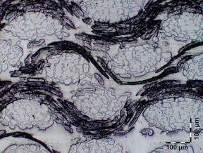
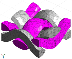
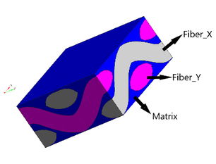
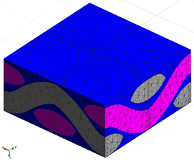
The micro-model developed to analyze the skin of the sandwich specimen is shown in Figure 4. The model has been developed in accordance with the microstructure observed in the same figure. The geometry has been meshed with four node tetrahedrons in a total of 9547 finite elements and 2287 nodes. The mesh can be seen in Figure 5.
|
|
3.2 Representative volume element of honeycomb
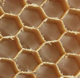
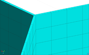
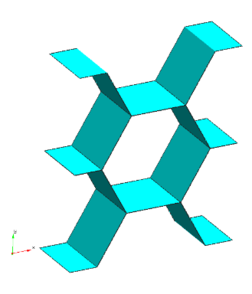
In order to numerically model the core of the sandwich panel a honeycomb RVE has been developed. The geometry together with a view of the real internal structure of the honeycomb can be observed in Figure 6. In Figure 7 the mesh used in the numerical simulation can be seen together with a zoom where the discretization in the thickness of the honeycomb wall can be observed. The geometry was meshed into 9600 linear hexahedral elements and 15666 nodes with two elements in the thickness direction of the honeycomb wall.
|

|
3.3 Results obtained from the numerical analysis
The simulation campaign began with simulations conducted on the two composing materials of the sandwich specimen separately in order to calibrate their mechanical properties. Results will be shown for the woven ramie rosin composite for the RR tensile test. The honeycomb has been calibrated to match the properties indicated in a standard data sheet. Finally, the results for the 4PB simulation will be shown.
3.3.1 Micro-model performance of woven ramie fibres in an epoxy matrix
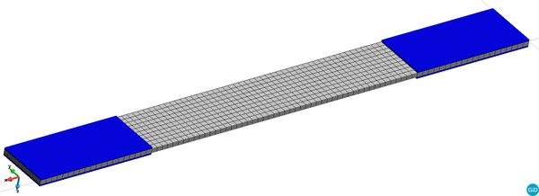
The behavior of the woven RR RVE has been analyzed by simulating a tensile test. The mesh used for the macro finite element model is shown in Figure 8. The mesh of the macromodel consists of 3500 linear hexahedral elements and 4928 nodes. At each integration point of the macro structure the woven RR RVE is computed in the first step of the linear domain.
The distribution of the main tensile stress is shown in Figure 9. The highest stress gradient can be seen, as expected, in the area closest to the tabs.
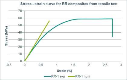
This simulation has been used in order to calibrate the properties of the woven ramie rosin composite in the elastic domain. The comparison of the stress - strain behaviour between the experimental result and the numerical one can be seen in Figure 10.
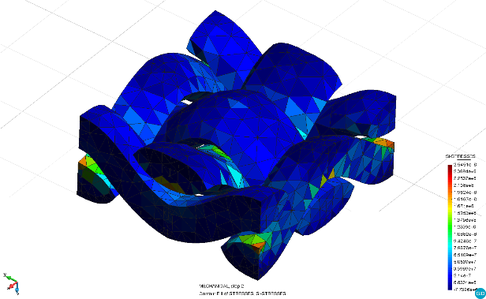
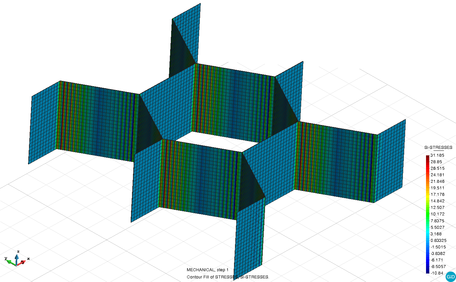
Figure 11 shows the distribution of the main tensile stress on the micromodel situated at one of the integration points of a FE situated in the proximity of the tabs. The result is shown only on the fibers that form the RVE. It can be seen that higher streeses develop in the fibers aligned with the loading direction on the macroscale, the x-x direction, as expected.
3.3.2 Micro-model performance of honeycomb
The behavior of the honeycomb RVE has also been studied in a different simulation. The macromodel consisted this time of only one linear hexahedral FE with 8 integration points. The movement of one face of the element has been restricted and a tensile displacement has been applied on its opposite face. At each of these integration points the honeycomb RVE has been computed. The material properties of the RVE are shown in Table 2. These values were calibrated to be same as the standard values available for a HexWeb A1 honeycomb.
| The RVE_02 Material properties | ||||
| Young Modulus (MPa) | Exx | Eyy | Ezz | |
| 34.88 | 35.10 | 138.31 | ||
| Shear Modulus (MPa) | Gxy | Gxz | Gyz | |
| 10.20 | 41.06 | 30.54 | ||
| Poisson Ratio | Pxy | Pyx | Pxz | |
| 0.5348 | 0.5313 | 0.3000 | ||
| Pzx | Pyz | Pzy | ||
| 0.0756 | 0.3000 | 0.0761 | ||
Figure 12 presents the distribution of the main tensile stresses on the honeycomb RVE.
3.3.3 4PB numerical simulation
With the material properties obtained from the two previously presented numerical simulations, the four point bending case has been analyzed.
At each integration point of the macro structure, either the woven RR RVE is computed if the element belongs to the skin, or the honeycomb RVE is computed if the element belongs to the core, in the first step of the linear domain.
After that, the RVE will be solved only on those integration points that exhibit stress states that surpass the elastic limit , in order to reduce computational time.
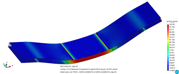
In Figure 13 the distribution of the main tensile stress can be seen on the deformed shape of the model for the two woven ramie rosin skins. As expected in a bending case, the tensile stresses appear on the inferior skin.
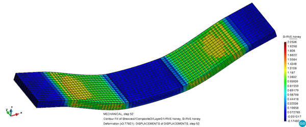
Figure 14 ehxibits the same result on the core of the sandwich where two symmetrical lateral areas are clearly marked as the most loaded ones.
Figure 15 shows the distribution of the internal damage variable on the model. Damage appears in the area where bending stresses develop and the pattern observed on the two faces of the model is a diagonal distribution that is found in shear failures. This is consistent with the failure mode observed in the experiment.
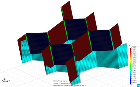
Figure 16 shows the distribution of the internal damage variable on the deformed shape of the honeycomb micromodel together with the initial undeformed mesh, for reference. The micromodel belongs to the integration point of the element where the maximum damage value appears in the macromodel, situated on the side of one of the flanks of the model.
Figure 16. Distribution of the internal damage variable on the honeycomb micromodel
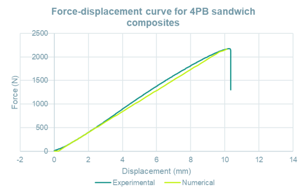
A comparison is made in Figure 17 between the behaviour of the model in the numerical simulation and in the experimental test in terms of the force – displacement curve. The reaction in the vertical direction is plotted versus the displacement of the node situated in the middle span of the specimen, on the inferior skin.
The correlation between the two curves is very good. However the numerical analysis can not capture the final abrupt failure due to loss of convergence.
4 Conclusions
This work has shown a numerical study conducted on a sandwich eco-composite using the multiscale analysis based on the classical first-order homogenization theory. Simulations have been conducted first on each of the composites forming the sandwich specimen in order to correctly asses their mechanical behavior and ensure an increased reliability of the simulation results.
The results of the four point bending simulation have been compared to experimental results in terms of failure mode and force - displacement curve and they have been found to be in good agreement.
It can be concluded that the multiscale numerical homogenization procedure is a valid and feasible method for the simulation of composites that have different complex microstructures, including in the nonlinear domain.
Aknowledgements
This work has been supported by the Spanish Ministerio de Economia y Competividad through the project BIAS2015-67807-R(RESCICLO) and by European Union EU-H2020 (Agreement No 690638)and the People’s Republic of China (Agreement No [2016]92)(ECOCOMPASS). All this support is gratefully acknowledged.
References
[() ] F. Otero, S.Oller, X. Martinez, Multiscale Computational Homogenization: Review and Proposal of a New Enhanced-First-Order Method, Archives of Computational Methods in Engineering 25, 2, 479-505 (2018). https://doi.org/10.1007/s11831-016-9205-0
[2] E. Car, S. Oller, E. Oñate, An anisotropic elastoplastic constitutive model for large strain analysis of fiber reinforced composite materials, Comput Methods Appl Mech Eng, 185 (2), pp. 245-277 (2000). 10.1016/S0045-7825(99)00262-5
[3] F. Rastellini, S. Oller, O. Salomón, E. Oñate, Composite materials non-linear modelling for long fibre-reinforced laminates: continuum basis, computational aspects and validations, Comput Struct, 86 (9), pp. 879-896, (2008). 10.1016/j.compstruc.2007.04.009
[4] A. Cornejo, L.G. Barbu, C. Escudero, X. Martínez, S. Oller, A.H. Barbat (2018). Methodology for the analysis of post-tensioned structures using a constitutive serial-parallel rule of mixtures. Composite Structures (2018); 200: 480-497. https://doi.org/10.1016/j.compstruct.2018.05.123
[5] S. Zaghi, X. Martinez, R. Rossi, M. Petracca, Adaptive and off-line techniques for non-linear multiscale analysis, Composite Structures, 206, pp 215-233 (2018). https://doi.org/10.1016/j.compstruct.2018.08.022.
[6] S. Ghosh, J. Bai, P. Raghavan Concurrent multi-level model for damage evolution in microstructurally debonding composites. Mech Mater 39(3):241–266 (2007) doi: 10.1016/j.mechmat.2006.05.004
[7] I. Gitman, H. Askes, L. Sluys Representative volume: existence and size determination. Eng Fract Mech 74(16):2518–2534 (2007). doi: 10.1016/j.engfracmech.2006.12.021
[8] S. Ilic, K. Hackl, Application of the multiscale FEM to the modeling of nonlinear multiphase materials. J Theor Appl Mech 47(3):537–551 (2009)
[9] N. Lahellec, P. Suquet, On the effective behavior of nonlinear inelastic composites: I. Incremental variational principles. J Mech Phys Solids 55(9):1932–1963 (2007). doi: 10.1016/j.jmps.2007.02.003
[10] S. Ghosh, K. Lee, P. Raghavan, A multi-level computational model for multi-scale damage analysis in composite and porous materials. Int J Solids Struct 38(14):2335–2385 (2001). doi: 10.1016/S0020-7683(00)00167-0
[11] R. Hill, A self-consistent mechanics of composite materials. J Mech Phys Solids 13(4):213–222 (1965). doi: 10.1016/0022-5096(65)90010-4
[12] JH Song, T. Belytschko, Multiscale aggregating discontinuities method for micro-macro failure of composites. Compos Part B Eng 40(6):417–426 (2009). doi: 10.1016/j.compositesb.2009.01.007
[13] K. Terada, N. Kikuchi, A class of general algorithms for multi-scale analyses of heterogeneous media. Comput Methods Appl Mech Eng 190(40–41):5427–5464 (2001). doi: 10.1016/S0045-7825(01)00179-7
[14] T. Kanit, S. Forest, I. Galliet, V. Mounoury, D. Jeulin, Determination of the size of the representative volume element for random composites: statistical and numerical approach. Int J Solids Struct 40(13–14):3647–3679 (2003). doi: 10.1016/S0020-7683(03)00143-4
[15] S. Giusti, P. Blanco, E. de Souza Neto, R. Feijó, An assessment of the Gurson yield criterion by a computational multi-scale approach. Eng Comput 26(3):281–301 (2009). doi: 10.1108/02644400910943626
[16] F. Otero, Multiscale numerical modelling of microstructured reinforced composites. Ph.D. thesis, Universitat Politècnica de Catalunya (BarcelonaTECH) (2016). doi: 10.13140/RG.2.1.5155.5600
[17] J. Bachmann, M. Wiedemann, P. Wierach, Flexural Mechanical Properties of Hybrid Epoxy Composites Reinforced with Nonwoven Made of Flax Fibres and Recycled Carbon Fibres. Aerospace 2018, 5(4), 107; https://doi.org/10.3390/aerospace5040107
[18] C. Miehe, Strain-driven homogenization of inelastic microstructures and composites based on an incremental variational formulation. Int J Numer Methods Eng 55(11):1285–1322 (2002). doi: 10.1002/nme.515
[19] I. Özdemir, W.A.M. Brekelmans, M.G.D. Geers, FE2 computational homogenization for the thermo-mechanical analysis of heterogeneous solids. Comput Methods Appl Mech Eng 198(3–4):602–613 (2008). doi: 10.1016/j.cma.2008.09.008
[20] D.D. Somer, E.A. de Souza Neto, W.G. Dettmer , D. Perić, A sub-stepping scheme for multi-scale analysis of solids. Comput Methods Appl Mech Eng 198(9–12):1006–1016 (2009). doi: 10.1016/j.cma.2008.11.013
[21] F. Otero, S. Oller, X. Martinez, O. Salomón, Numerical homogenization for composite materials analysis. Comparison with other micro mechanical formulations. Compos Struct 122:405–416 (2015). doi: 10.1016/j.compstruct.2014.11.041
[22] P.M. Suquet, Local and global aspects in the mathematical theory of plasticity Plasticity Today, 5, pp. 279-309 (1985),
[URL:https://ci.nii.ac.jp/naid/10009833388/en/ URL:https://ci.nii.ac.jp/naid/10009833388/en/]
[23] J. Hernández, J. Oliver, A. Huespe, M. Caicedo-Silva, J. Cante,
High-performance model reduction techniques in computational multiscale homogenization Comput Methods Appl Mech Eng, 276, pp. 149-189 (2014)
Document information
Published on 01/06/22
Accepted on 29/05/22
Submitted on 28/05/22
Volume 04 - Comunicaciones Matcomp19 (2020), Issue Núm. 1 - Avances en Materiales Compuestos. Nuevos Campos de Aplicación., 2022
DOI: 10.23967/r.matcomp.2022.06.001
Licence: Other
Share this document
Keywords
claim authorship
Are you one of the authors of this document?

