m (Lfvm94 moved page Review 975456380192 to Draft Verduzco Martinez 342172656) |
|||
| Line 32: | Line 32: | ||
{| class="floating_imageSCP" style="text-align: center; border: 1px solid #BBB; margin: 1em auto; width: 100%;max-width: 100%;" | {| class="floating_imageSCP" style="text-align: center; border: 1px solid #BBB; margin: 1em auto; width: 100%;max-width: 100%;" | ||
|- | |- | ||
| − | |[[Image: | + | |[[Image:Draft_Verduzco Martinez_342172656-sys_flow_rc.png|422px|System flow for the area of optimization in RC structures,<span id='citeF-15'></span>[[#cite-15|[15]]].]] |
|- style="text-align: center; font-size: 75%;" | |- style="text-align: center; font-size: 75%;" | ||
| colspan="1" | '''Figure 1:''' System flow for the area of optimization in RC structures,<span id='citeF-15'></span>[[#cite-15|[15]]]. | | colspan="1" | '''Figure 1:''' System flow for the area of optimization in RC structures,<span id='citeF-15'></span>[[#cite-15|[15]]]. | ||
| Line 44: | Line 44: | ||
{| class="floating_imageSCP" style="text-align: center; border: 1px solid #BBB; margin: 1em auto; width: 100%;max-width: 100%;" | {| class="floating_imageSCP" style="text-align: center; border: 1px solid #BBB; margin: 1em auto; width: 100%;max-width: 100%;" | ||
|- | |- | ||
| − | |[[Image: | + | |[[Image:Draft_Verduzco Martinez_342172656-rsd.png|271px|A typical Reinforcement Sizing Diagram for a given load combination. <span id='citeF-5'></span>[[#cite-5|[5]]]]] |
|- style="text-align: center; font-size: 75%;" | |- style="text-align: center; font-size: 75%;" | ||
| colspan="1" | '''Figure 2:''' A typical Reinforcement Sizing Diagram for a given load combination. <span id='citeF-5'></span>[[#cite-5|[5]]] | | colspan="1" | '''Figure 2:''' A typical Reinforcement Sizing Diagram for a given load combination. <span id='citeF-5'></span>[[#cite-5|[5]]] | ||
| Line 55: | Line 55: | ||
{| class="floating_imageSCP" style="text-align: center; border: 1px solid #BBB; margin: 1em auto; width: 100%;max-width: 100%;" | {| class="floating_imageSCP" style="text-align: center; border: 1px solid #BBB; margin: 1em auto; width: 100%;max-width: 100%;" | ||
|- | |- | ||
| − | |[[Image: | + | |[[Image:Draft_Verduzco Martinez_342172656-lcrd.png|302px|]] |
| − | |[[Image: | + | |[[Image:Draft_Verduzco Martinez_342172656-section_lcrd.png|182px|A typical Load Combination Reinforcement Diagram at the left and its corresponding reinforced cross section element from which Aₛ and A<sup>'</sup>ₛ are taken as smeared reinforcement steel. <span id='citeF-7'></span>[[#cite-7|[7]]]]] |
|- style="text-align: center; font-size: 75%;" | |- style="text-align: center; font-size: 75%;" | ||
| colspan="2" | '''Figure 3:''' A typical Load Combination Reinforcement Diagram at the left and its corresponding reinforced cross section element from which <math>A_{s}</math> and <math>A^{'}_{s}</math> are taken as smeared reinforcement steel. <span id='citeF-7'></span>[[#cite-7|[7]]] | | colspan="2" | '''Figure 3:''' A typical Load Combination Reinforcement Diagram at the left and its corresponding reinforced cross section element from which <math>A_{s}</math> and <math>A^{'}_{s}</math> are taken as smeared reinforcement steel. <span id='citeF-7'></span>[[#cite-7|[7]]] | ||
| Line 66: | Line 66: | ||
{| class="floating_imageSCP" style="text-align: center; border: 1px solid #BBB; margin: 1em auto; width: 100%;max-width: 100%;" | {| class="floating_imageSCP" style="text-align: center; border: 1px solid #BBB; margin: 1em auto; width: 100%;max-width: 100%;" | ||
|- | |- | ||
| − | |[[Image: | + | |[[Image:Draft_Verduzco Martinez_342172656-steel_plates.png|207px|Idealization of reinforcing steel proposed by <span id='citeF-8'></span>[[#cite-8|[8]]] for each axis direction of a rectangular column.]] |
|- style="text-align: center; font-size: 75%;" | |- style="text-align: center; font-size: 75%;" | ||
| colspan="1" | '''Figure 4:''' Idealization of reinforcing steel proposed by <span id='citeF-8'></span>[[#cite-8|[8]]] for each axis direction of a rectangular column. | | colspan="1" | '''Figure 4:''' Idealization of reinforcing steel proposed by <span id='citeF-8'></span>[[#cite-8|[8]]] for each axis direction of a rectangular column. | ||
| Line 76: | Line 76: | ||
{| class="floating_imageSCP" style="text-align: center; border: 1px solid #BBB; margin: 1em auto; width: 100%;max-width: 100%;" | {| class="floating_imageSCP" style="text-align: center; border: 1px solid #BBB; margin: 1em auto; width: 100%;max-width: 100%;" | ||
|- | |- | ||
| − | |[[Image: | + | |[[Image:Draft_Verduzco Martinez_342172656-inclined_crossection.png|166px|General formulation reference of cross section for the analysis and calculation of resistance of a reinforced concrete element. <span id='citeF-9'></span>[[#cite-9|[9]]]]] |
|- style="text-align: center; font-size: 75%;" | |- style="text-align: center; font-size: 75%;" | ||
| colspan="1" | '''Figure 5:''' General formulation reference of cross section for the analysis and calculation of resistance of a reinforced concrete element. <span id='citeF-9'></span>[[#cite-9|[9]]] | | colspan="1" | '''Figure 5:''' General formulation reference of cross section for the analysis and calculation of resistance of a reinforced concrete element. <span id='citeF-9'></span>[[#cite-9|[9]]] | ||
| Line 84: | Line 84: | ||
{| class="floating_imageSCP" style="text-align: center; border: 1px solid #BBB; margin: 1em auto; width: 100%;max-width: 100%;" | {| class="floating_imageSCP" style="text-align: center; border: 1px solid #BBB; margin: 1em auto; width: 100%;max-width: 100%;" | ||
|- | |- | ||
| − | |[[Image: | + | |[[Image:Draft_Verduzco Martinez_342172656-contourplot_minimumarea.png|399px|Contour graph for minimum reinforcement area corresponding to different values of ξ and ϕ. <span id='citeF-9'></span>[[#cite-9|[9]]]]] |
|- style="text-align: center; font-size: 75%;" | |- style="text-align: center; font-size: 75%;" | ||
| colspan="1" | '''Figure 6:''' Contour graph for minimum reinforcement area corresponding to different values of <math>\xi </math> and <math>\phi </math>. <span id='citeF-9'></span>[[#cite-9|[9]]] | | colspan="1" | '''Figure 6:''' Contour graph for minimum reinforcement area corresponding to different values of <math>\xi </math> and <math>\phi </math>. <span id='citeF-9'></span>[[#cite-9|[9]]] | ||
| Line 96: | Line 96: | ||
{| class="floating_imageSCP" style="text-align: center; border: 1px solid #BBB; margin: 1em auto; width: 100%;max-width: 100%;" | {| class="floating_imageSCP" style="text-align: center; border: 1px solid #BBB; margin: 1em auto; width: 100%;max-width: 100%;" | ||
|- | |- | ||
| − | |[[Image: | + | |[[Image:Draft_Verduzco Martinez_342172656-Fig6.png|129px|]] |
| − | |[[Image: | + | |[[Image:Draft_Verduzco Martinez_342172656-fig23.png|181px|The ''“Idealized Steel Profile”'' method <span id='citeF-12'></span>[[#cite-12|[12]]] for rectangular and circular solid cross sectioned concrete elements]] |
|- style="text-align: center; font-size: 75%;" | |- style="text-align: center; font-size: 75%;" | ||
| colspan="2" | '''Figure 7:''' The ''“Idealized Steel Profile”'' method <span id='citeF-12'></span>[[#cite-12|[12]]] for rectangular and circular solid cross sectioned concrete elements | | colspan="2" | '''Figure 7:''' The ''“Idealized Steel Profile”'' method <span id='citeF-12'></span>[[#cite-12|[12]]] for rectangular and circular solid cross sectioned concrete elements | ||
| Line 109: | Line 109: | ||
{| class="floating_imageSCP" style="text-align: center; border: 1px solid #BBB; margin: 1em auto; width: 100%;max-width: 100%;" | {| class="floating_imageSCP" style="text-align: center; border: 1px solid #BBB; margin: 1em auto; width: 100%;max-width: 100%;" | ||
|- | |- | ||
| − | |[[Image: | + | |[[Image:Draft_Verduzco Martinez_342172656-probform.png|334px|Reference system for the rotation of a rectangular cross-section when computing a surface diagram. <span id='citeF-9'></span>[[#cite-9|[9]]]]] |
|- style="text-align: center; font-size: 75%;" | |- style="text-align: center; font-size: 75%;" | ||
| colspan="1" | '''Figure 8:''' Reference system for the rotation of a rectangular cross-section when computing a surface diagram. <span id='citeF-9'></span>[[#cite-9|[9]]] | | colspan="1" | '''Figure 8:''' Reference system for the rotation of a rectangular cross-section when computing a surface diagram. <span id='citeF-9'></span>[[#cite-9|[9]]] | ||
| Line 127: | Line 127: | ||
{| class="floating_imageSCP" style="text-align: center; border: 1px solid #BBB; margin: 1em auto; width: 100%;max-width: 100%;" | {| class="floating_imageSCP" style="text-align: center; border: 1px solid #BBB; margin: 1em auto; width: 100%;max-width: 100%;" | ||
|- | |- | ||
| − | |[[Image: | + | |[[Image:Draft_Verduzco Martinez_342172656-diagintreferencia.png|341px|Reference system for the determination of structural efficiency of a any flexure compression condition]] |
|- style="text-align: center; font-size: 75%;" | |- style="text-align: center; font-size: 75%;" | ||
| colspan="1" | '''Figure 9:''' Reference system for the determination of structural efficiency of a any flexure compression condition | | colspan="1" | '''Figure 9:''' Reference system for the determination of structural efficiency of a any flexure compression condition | ||
| Line 152: | Line 152: | ||
{| class="floating_imageSCP" style="text-align: center; border: 1px solid #BBB; margin: 1em auto; width: 100%;max-width: 100%;" | {| class="floating_imageSCP" style="text-align: center; border: 1px solid #BBB; margin: 1em auto; width: 100%;max-width: 100%;" | ||
|- | |- | ||
| − | |[[Image: | + | |[[Image:Draft_Verduzco Martinez_342172656-efficiency_function_single_t.png|252px|Behaviour of the Efficiency function of a single width value (t) of the ISR]] |
|- style="text-align: center; font-size: 75%;" | |- style="text-align: center; font-size: 75%;" | ||
| colspan="1" | '''Figure 10:''' Behaviour of the Efficiency function of a single width value (t) of the ISR | | colspan="1" | '''Figure 10:''' Behaviour of the Efficiency function of a single width value (t) of the ISR | ||
| Line 162: | Line 162: | ||
{| class="floating_imageSCP" style="text-align: center; border: 1px solid #BBB; margin: 1em auto; width: 100%;max-width: 100%;" | {| class="floating_imageSCP" style="text-align: center; border: 1px solid #BBB; margin: 1em auto; width: 100%;max-width: 100%;" | ||
|- | |- | ||
| − | |[[Image: | + | |[[Image:Draft_Verduzco Martinez_342172656-fig12.png|295px|Mathematical formulation fo the ISR method. Ideal for computational saving applied to rectangular cross-sections]] |
|- style="text-align: center; font-size: 75%;" | |- style="text-align: center; font-size: 75%;" | ||
| colspan="1" | '''Figure 11:''' Mathematical formulation fo the ISR method. Ideal for computational saving applied to rectangular cross-sections | | colspan="1" | '''Figure 11:''' Mathematical formulation fo the ISR method. Ideal for computational saving applied to rectangular cross-sections | ||
| Line 170: | Line 170: | ||
{| class="floating_imageSCP" style="text-align: center; border: 1px solid #BBB; margin: 1em auto; width: 100%;max-width: 100%;" | {| class="floating_imageSCP" style="text-align: center; border: 1px solid #BBB; margin: 1em auto; width: 100%;max-width: 100%;" | ||
|- | |- | ||
| − | |[[Image: | + | |[[Image:Draft_Verduzco Martinez_342172656-fig27.png|249px|Discrete formulation for the ISR method for circular cross-sections. Ideal for complex geometries.]] |
|- style="text-align: center; font-size: 75%;" | |- style="text-align: center; font-size: 75%;" | ||
| colspan="1" | '''Figure 12:''' Discrete formulation for the ISR method for circular cross-sections. Ideal for complex geometries. | | colspan="1" | '''Figure 12:''' Discrete formulation for the ISR method for circular cross-sections. Ideal for complex geometries. | ||
| Line 217: | Line 217: | ||
{| class="floating_imageSCP" style="text-align: center; border: 1px solid #BBB; margin: 1em auto; width: 100%;max-width: 100%;" | {| class="floating_imageSCP" style="text-align: center; border: 1px solid #BBB; margin: 1em auto; width: 100%;max-width: 100%;" | ||
|- | |- | ||
| − | |[[Image: | + | |[[Image:Draft_Verduzco Martinez_342172656-steepest_descent_form.png|309px|Slope criteria for the Steepest Descent Optimization Method formulation.]] |
|- style="text-align: center; font-size: 75%;" | |- style="text-align: center; font-size: 75%;" | ||
| colspan="1" | '''Figure 13:''' Slope criteria for the Steepest Descent Optimization Method formulation. | | colspan="1" | '''Figure 13:''' Slope criteria for the Steepest Descent Optimization Method formulation. | ||
| Line 485: | Line 485: | ||
{| class="floating_imageSCP" style="text-align: center; border: 1px solid #BBB; margin: 1em auto; width: 100%;max-width: 100%;" | {| class="floating_imageSCP" style="text-align: center; border: 1px solid #BBB; margin: 1em auto; width: 100%;max-width: 100%;" | ||
|- | |- | ||
| − | |[[Image: | + | |[[Image:Draft_Verduzco Martinez_342172656-evolution_area_iteration.png|224px|Progression of reinforcing area for each iteration of the PSO-ISR algorithm]] |
|- style="text-align: center; font-size: 75%;" | |- style="text-align: center; font-size: 75%;" | ||
| colspan="1" | '''Figure 14:''' Progression of reinforcing area for each iteration of the PSO-ISR algorithm | | colspan="1" | '''Figure 14:''' Progression of reinforcing area for each iteration of the PSO-ISR algorithm | ||
| Line 497: | Line 497: | ||
{| class="floating_imageSCP" style="text-align: center; border: 1px solid #BBB; margin: 1em auto; width: 100%;max-width: 100%;" | {| class="floating_imageSCP" style="text-align: center; border: 1px solid #BBB; margin: 1em auto; width: 100%;max-width: 100%;" | ||
|- | |- | ||
| − | |[[Image: | + | |[[Image:Draft_Verduzco Martinez_342172656-diagPerfil4t_X.png|224px|Interaction diagram in the X-axis direction for the global optima 4t-ISR]] |
|- style="text-align: center; font-size: 75%;" | |- style="text-align: center; font-size: 75%;" | ||
| colspan="1" | '''Figure 15:''' Interaction diagram in the X-axis direction for the global optima 4t-ISR | | colspan="1" | '''Figure 15:''' Interaction diagram in the X-axis direction for the global optima 4t-ISR | ||
| Line 505: | Line 505: | ||
{| class="floating_imageSCP" style="text-align: center; border: 1px solid #BBB; margin: 1em auto; width: 100%;max-width: 100%;" | {| class="floating_imageSCP" style="text-align: center; border: 1px solid #BBB; margin: 1em auto; width: 100%;max-width: 100%;" | ||
|- | |- | ||
| − | |[[Image: | + | |[[Image:Draft_Verduzco Martinez_342172656-diagPerfil4t_Y.png|224px|Interaction diagram in the Y-axis direction for the global optima 4t-ISR]] |
|- style="text-align: center; font-size: 75%;" | |- style="text-align: center; font-size: 75%;" | ||
| colspan="1" | '''Figure 16:''' Interaction diagram in the Y-axis direction for the global optima 4t-ISR | | colspan="1" | '''Figure 16:''' Interaction diagram in the Y-axis direction for the global optima 4t-ISR | ||
| Line 533: | Line 533: | ||
{| class="floating_imageSCP" style="text-align: center; border: 1px solid #BBB; margin: 1em auto; width: 100%;max-width: 100%;" | {| class="floating_imageSCP" style="text-align: center; border: 1px solid #BBB; margin: 1em auto; width: 100%;max-width: 100%;" | ||
|- | |- | ||
| − | |[[Image: | + | |[[Image:Draft_Verduzco Martinez_342172656-GA-ISR-evolution_area.png|224px|Evolution of the optimal reinforcing area with the GA-ISR]] |
|- style="text-align: center; font-size: 75%;" | |- style="text-align: center; font-size: 75%;" | ||
| colspan="1" | '''Figure 17:''' Evolution of the optimal reinforcing area with the GA-ISR | | colspan="1" | '''Figure 17:''' Evolution of the optimal reinforcing area with the GA-ISR | ||
| Line 543: | Line 543: | ||
{| class="floating_imageSCP" style="text-align: center; border: 1px solid #BBB; margin: 1em auto; width: 100%;max-width: 100%;" | {| class="floating_imageSCP" style="text-align: center; border: 1px solid #BBB; margin: 1em auto; width: 100%;max-width: 100%;" | ||
|- | |- | ||
| − | |[[Image: | + | |[[Image:Draft_Verduzco Martinez_342172656-diagIntXGA.png|224px|Interaction diagram in the X-axis direction for the global optima 4t-ISR-GA]] |
|- style="text-align: center; font-size: 75%;" | |- style="text-align: center; font-size: 75%;" | ||
| colspan="1" | '''Figure 18:''' Interaction diagram in the X-axis direction for the global optima 4t-ISR-GA | | colspan="1" | '''Figure 18:''' Interaction diagram in the X-axis direction for the global optima 4t-ISR-GA | ||
| Line 551: | Line 551: | ||
{| class="floating_imageSCP" style="text-align: center; border: 1px solid #BBB; margin: 1em auto; width: 100%;max-width: 100%;" | {| class="floating_imageSCP" style="text-align: center; border: 1px solid #BBB; margin: 1em auto; width: 100%;max-width: 100%;" | ||
|- | |- | ||
| − | |[[Image: | + | |[[Image:Draft_Verduzco Martinez_342172656-diagIntYGA.png|224px|Interaction diagram in the Y-axis direction for the global optima 4t-ISR-GA]] |
|- style="text-align: center; font-size: 75%;" | |- style="text-align: center; font-size: 75%;" | ||
| colspan="1" | '''Figure 19:''' Interaction diagram in the Y-axis direction for the global optima 4t-ISR-GA | | colspan="1" | '''Figure 19:''' Interaction diagram in the Y-axis direction for the global optima 4t-ISR-GA | ||
| Line 907: | Line 907: | ||
{| class="floating_imageSCP" style="text-align: center; border: 1px solid #BBB; margin: 1em auto; width: 100%;max-width: 100%;" | {| class="floating_imageSCP" style="text-align: center; border: 1px solid #BBB; margin: 1em auto; width: 100%;max-width: 100%;" | ||
|- | |- | ||
| − | |[[Image: | + | |[[Image:Draft_Verduzco Martinez_342172656-Graph_SGD_1t.png|224px|Convergence of the Steepest Gradient Descent method for the 1t-ISR]] |
|- style="text-align: center; font-size: 75%;" | |- style="text-align: center; font-size: 75%;" | ||
| colspan="1" | '''Figure 20:''' Convergence of the Steepest Gradient Descent method for the 1t-ISR | | colspan="1" | '''Figure 20:''' Convergence of the Steepest Gradient Descent method for the 1t-ISR | ||
| Line 915: | Line 915: | ||
{| class="floating_imageSCP" style="text-align: center; border: 1px solid #BBB; margin: 1em auto; width: 100%;max-width: 100%;" | {| class="floating_imageSCP" style="text-align: center; border: 1px solid #BBB; margin: 1em auto; width: 100%;max-width: 100%;" | ||
|- | |- | ||
| − | |[[Image: | + | |[[Image:Draft_Verduzco Martinez_342172656-1t_SGD_diagIntX.png|224px|Interaction diagram in the X-axis direction for the global optima 4t-ISR-GA]] |
|- style="text-align: center; font-size: 75%;" | |- style="text-align: center; font-size: 75%;" | ||
| colspan="1" | '''Figure 21:''' Interaction diagram in the X-axis direction for the global optima 4t-ISR-GA | | colspan="1" | '''Figure 21:''' Interaction diagram in the X-axis direction for the global optima 4t-ISR-GA | ||
| Line 923: | Line 923: | ||
{| class="floating_imageSCP" style="text-align: center; border: 1px solid #BBB; margin: 1em auto; width: 100%;max-width: 100%;" | {| class="floating_imageSCP" style="text-align: center; border: 1px solid #BBB; margin: 1em auto; width: 100%;max-width: 100%;" | ||
|- | |- | ||
| − | |[[Image: | + | |[[Image:Draft_Verduzco Martinez_342172656-1t_SGD_diagIntY.png|224px|Interaction diagram in the X-axis direction for the global optima 4t-ISR-GA]] |
|- style="text-align: center; font-size: 75%;" | |- style="text-align: center; font-size: 75%;" | ||
| colspan="1" | '''Figure 22:''' Interaction diagram in the X-axis direction for the global optima 4t-ISR-GA | | colspan="1" | '''Figure 22:''' Interaction diagram in the X-axis direction for the global optima 4t-ISR-GA | ||
| Line 1,036: | Line 1,036: | ||
{| class="floating_imageSCP" style="text-align: center; border: 1px solid #BBB; margin: 1em auto; width: 100%;max-width: 100%;" | {| class="floating_imageSCP" style="text-align: center; border: 1px solid #BBB; margin: 1em auto; width: 100%;max-width: 100%;" | ||
|- | |- | ||
| − | |[[Image: | + | |[[Image:Draft_Verduzco Martinez_342172656-4t-isr-topologies.png|447px|Transformation from the 4t-ISR formulation to reinforcing bars.]] |
|- style="text-align: center; font-size: 75%;" | |- style="text-align: center; font-size: 75%;" | ||
| colspan="1" | '''Figure 23:''' Transformation from the 4t-ISR formulation to reinforcing bars. | | colspan="1" | '''Figure 23:''' Transformation from the 4t-ISR formulation to reinforcing bars. | ||
Revision as of 02:29, 8 January 2021
Abstract
The present work aims to define formally the method termed as “Idealized Smeared Reinforcement” (ISR) for optimization in the design of reinforcing steel in concrete structures, its boundaries, background and potentials. Such method has been extensively used implicitly in many different studies of reinforced concrete structures related with optimization and mechanical structural behaviour, but it has not yet been formally established as a method itself even though it represents a great solution approach when designing optimally concrete sections, which is a tendency so vital nowadays for sustainability in construction projects. A general survey of such method of the ISR will be presented on in this document, presenting relevant background research related to the use of the method and optimization of reinforcing steel in general for concrete structures, thereafter proposals of different optimization methods, both classical optimization and meta-heuristic methods will be regarded as possible approaches to apply the ISR, specifically Gradient Descent Optimization methods when one variable for the ISR is considered and meta-heuristics for more than one variable involved given their versatility and flexibility to adapt to different problems, particularly the Particle Swarm Optimization PSO method and the Genetic Algorithm GA. At the end, these solution approaches for the application of the ISR method will be compared for the testing of rectangular solid geometries with different analysis parameters in order to show how adaptable and feasible such ISR method might be using a proper optimization algorithm and analysis for its approach when designing reinforcing steel.
1 Introduction
Ever since Whitney and Cohen [2] many years ago in 1956 proposed a guide to design reinforcing steel in concrete structures subject to axial force and bending moment by ultimate strength based on the ACI code many different approaches have taken place from that point on to design optimally reinforced concrete sections. What Whitney and Cohen presented then was a series of charts based on N-M interaction diagrams normalized considering symmetric and uniform reinforcement over a cross section. In recent years however, new more realistic considerations for the design and analysis have been carried on, for instance, influence of confinement and flexural behaviour [3], or non-symmetric reinforcement [4] in which a particular solution of a problem is provided for elements subjected to flexure-compression stresses. Also, the concept of strength design has been challenged by new design approaches [5] which generate a family of solutions for arbitrary combinations of imposed axial load and moment, requiring even a non-symmetric distribution of reinforcement over the cross section. Moreover, theorems for optimal section reinforcement have been also developed [6] based on the understanding of all these studied optimal solutions, encompassing a general formulation to determine the minimum total reinforcement area required for adequate resistance to axial load and moment.
Through all of these conducted research works the idealization of a continous distributed plate along the faces of a rectangular cross section has already been created. But it is specifically in [9] by Anschheim et. al. when the concept of a “Smeared reinforcement” idealization is given formally, in which an optimization for the values of each of the four continuous plates areas (smeared reinforcement) distributed over a rectangular cross section (upper, lower, right and left faces) is carried on, establishing its due design restrictions according to the ACI-318 code, thus finding minimum reinforcement required areas for a given load combination related to the orientation of the axis direction of the cross section geometry. In recent years, this very approach made by officially by Anschheim et. al. in 2008 has also been carried on by other authors [12] although differing by means of solutions generated or by the analysis method itself.
L. Verduzco [12] made a research related directly with this very topic in which a called “Idealized Steel Profile” concept was introduced, idealizing the reinforcement steel as a continuous steel PTR structural profile embedded into the concrete element with a uniform width from which an optimization analysis was carried on to seek an optimal arrangement of reinforcing steel bars over the cross section element (either the most economical or structurally efficient), with certain restrictions such as equal diameter for the reinforcing bars according to the normative of the region. What it is also relevant to stress from this research is the purely mathematical analysis approach that was made, by defining blocks of stress and strain over the section as the depth value of the neutral axis varies, thus defining equations of resistance for different cases in which the neutral axis depth might have been located. While on one hand Anschheim et. al. generated a family of solutions given by means of percentage of reinforcing steel with respect of the cross section element net area, on the other L. Verduzco designed a mathematical approach through a computational optimization method to seek an optimal reinforcement area from which to transform directly to reinforcing steel bars arrangements. Even though both approaches differ one from another, the idea is the same, and it is of special importance to promote this concept and method by giving it a whole research work focused on its boundaries, limitations, potentials, different possible analysis and optimization approaches.
This very optimization domain presented hereby for RC structures design corresponds to a vital element of the systematic flow of research for RC structures suggested in various literature [15] Fig. 1 in which this problem is directly related to the stage of “Integration of promising techniques” for the improvement of performance of optimization strategies in detailed design of RC structures. Therefore, it can be justified from this perspective the importance and relevance of this such research work, to strengthen this very scenario for optimization in RC structures.
![System flow for the area of optimization in RC structures,[15].](/wd/images/thumb/5/55/Draft_Verduzco_Martinez_342172656-sys_flow_rc.png/422px-Draft_Verduzco_Martinez_342172656-sys_flow_rc.png)
|
| Figure 1: System flow for the area of optimization in RC structures,[15]. |
2 Background
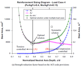
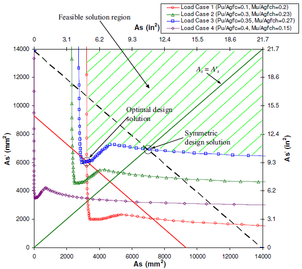
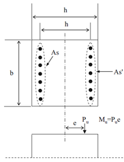
Resuming the content of the most recent research related with optimization of reinforcing steel, it is of vital relevance to stress the development and introduction of a so called Reinforcement Sizing Diagram (RSD), formulated in [5], which displays a minimum required steel reinforcement area in one axis for a respective neutral axis depth in the other axis, given a combination of axial load and moment Fig. 2. Another relevant development is the called ``Load Combination Reinforcement Diagram (LCRD) [7] which on the other hand plots reinforcement solutions in a two-dimensional space Fig. 3a (left) defined by the coordinates corresponding to the reinforcement area on each of the faces of a rectangular cross section element Fig. 3 (right) allowing an engineer to easily determine an optimal reinforcement solution from given load combinations on structural concrete elements subject to biaxial flexure-compression stresses. Such (LCRD) are obtained by collecting different values of reinforcement area from a (RSD) corresponding to different values of the axis depth . It is what in multi-objective optimization would be called a Pareto Front.
 ] ]
|
| Figure 2: A typical Reinforcement Sizing Diagram for a given load combination. [5] |
It is important to stress that in the development of the LCRD was also introduced the concept of asymmetrical reinforcement uniformity over an element cross-section, based on studies which concluded that for optimal solutions an asymmetric distribution of reinforcing steel was more likely to take place [7], therefore different faces of an element cross-section were picked to assign them different values of reinforcing steel area, as seen in Fig. 3 (right), and to have a better approximation for a minimum required reinforcement, taking reference from the such smeared reinforcement concept made firstly in [9].
|
 ] ]
|
| Figure 3: A typical Load Combination Reinforcement Diagram at the left and its corresponding reinforced cross section element from which and are taken as smeared reinforcement steel. [7] | |
Such diagrams have been used in many further research works [8], in which even though the typical approaches and hypotheses first formulated many years ago to design reinforced concrete sections [10], [11] (for rectangular geometries) are still taken on account, other different assumptions are carried on in order to optimize the reinforcing steel, such as asymmetric reinforcement following the research made by [9] as well Fig. 4, but focusing merely on design outcomes, addressing more flexible design considerations.
![Idealization of reinforcing steel proposed by [8] for each axis direction of a rectangular column.](/wd/images/thumb/9/95/Draft_Verduzco_Martinez_342172656-steel_plates.png/207px-Draft_Verduzco_Martinez_342172656-steel_plates.png)
|
| Figure 4: Idealization of reinforcing steel proposed by [8] for each axis direction of a rectangular column. |
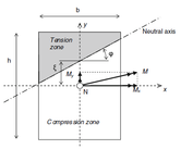
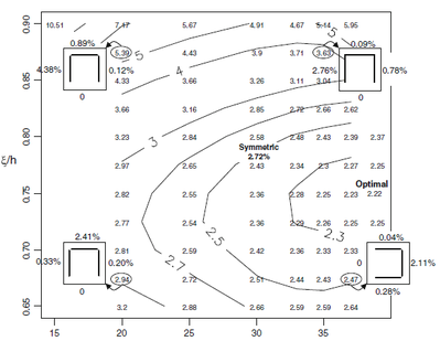
Aschheim et. al. [9] used non-linear conjugate gradient search methods to obtain optimal solutions for these such mentioned smeared reinforcing steel areas, applied to a structural model for different values of rotation of the structural rectangular cross section and ratio between axial force and bending moment Fig. 5. The results generated were plotted in a contour graph Fig. 6 for the minimum reinforcement areas thereby found, by means of steel area percentage in relation with the concrete area, which may be of great use to standardize design precesses.
 ] ]
|
| Figure 5: General formulation reference of cross section for the analysis and calculation of resistance of a reinforced concrete element. [9] |
 ] ]
|
| Figure 6: Contour graph for minimum reinforcement area corresponding to different values of and . [9] |
Based on this contour graphs, or for the generation of such, constraints may be imposed regarding the type of reinforcement sought (symmetrical or non-symmetrical) either for all faces or opposite ones. By setting equal values of and corresponding to reinforcement areas on opposite faces, two variables to minimize are obtain, or on the other hand, by setting all areas equal to one another obtaining only one variable to minimize. This method of optimization is capable of saving as much as up to 10% in relation with the conventional methods for design and conventional restrictions for reinforced columns of symmetric and uniform steel reinforcement based on the [1] code, depending also on the decision made by the engineer or contractor.
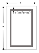
Regarding other optimization approaches L.Verduzco [12] idealization of the such mentioned “Smeared reinforcement” as a continuous steel structural profile of uniform width which he referred to as ``The Idealized Steel Profile, embedded into a concrete element from which a mathematical approach was carried on through a constant length step computational optimization method for both rectangular and circular solid cross sections Fig. 7 presented advantages of execution time when big geometries are analysed, due to the mathematical analysis in which only a few conditions and operations are required in order to calculate the resistance of a given value of (steel profile width) for a respective depth of the neutral axis. Even though such mathematical approach may not be quite applicable to circular cross sections due to the complexity it enhances in the analysis. For designs fully based on normative where so many restrictions are imposed this approach might be of great potential for any geometry, the problem comes up when seeking optimal unsymmetrical reinforcement when a bending moment condition is significantly mayor for one of the axis in a rectangular section, for which such uniform idealization of steel does not really guarantee a good approximation for the required reinforcement area due tu the constant variation of the width on both axis directions.
|
![The “Idealized Steel Profile” method [12] for rectangular and circular solid cross sectioned concrete elements](/wd/images/thumb/8/87/Draft_Verduzco_Martinez_342172656-fig23.png/181px-Draft_Verduzco_Martinez_342172656-fig23.png)
|
| Figure 7: The “Idealized Steel Profile” method [12] for rectangular and circular solid cross sectioned concrete elements | |
3 Analysis approaches for optimization with the ISR
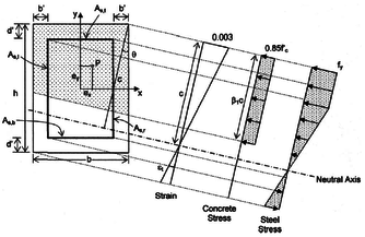
Different formulations for the analysis of a problem with the ISR method might be carried on, either regarding mechanical analysis (flexure-compression for short or slender elements) possibly using the Bresler's formula [10] or by computing an interaction surface diagram by rotating the cross section element Fig. 8 on its own longitudinal axis (depending on the required approximation accuracy); or with relation of the optimization analysis approach adopted, merely with classical optimization or mathematical programming methods, such as Gradient Descent Based methods as formulated by Anschheim et. al. [9] for two steel area values (or variables), or when using the Idealized Steel Profile proposed by L. Verduzco [12] for only one variable a simple numeric search method might be feasible for small cross section columns. Meta-heuristic algorithms of optimization might also be viable to adopt, for instance, taking Evolutionary Algorithms, Swarm Algorithms, Multi-objective optimization and such. Meta-heuristic optimization algorithms might be more feasible than classical optimization methods when formulating more than one different steel area values or when massive cross section elements take place, given the complexity a mathematical optimization approach may enhance.
 ] ]
|
| Figure 8: Reference system for the rotation of a rectangular cross-section when computing a surface diagram. [9] |
There has also been research and development regarding general theorems for an optimal reinforcement design [6], based on all of the research previously mentioned involving the idealization of Smeared Reinforcement, which states that the minimum total required reinforcement area for adequate resistance to axial load and moment can be identified as the minimum admissible solution among five discrete analysis cases from the infinite set of potential solutions. Such theorem is of great potential when designing for common parameters most often used in structural engineering practice and it is also of importance to mention its existence.
3.1 Optimization approaches for the ISR method
As following, different optimization methods of possible potential for the application of the ISR, such as the Particle Swarm Optimization Algorithm along with the GA for multiple values of width to optimize, the Multiple Linear Regression method for a single variable of width to estimate an initial value of with from which to start iterating in a Simple search1 to get to the required structural efficiency without a complicated formulation, but only with experimentation and collection of data. optimization method, as well as a Gradient Descent Method are carried on and compared. It was considered that meta-heuristic algorithms could be of greater potential for this engineering problem rather than classical optimization methods, such as Newton-Raphson or a Gradient Descent Based Method given the complexity of analysis they imply when formulating a problem for more than 2 variables on place which are more needed when the steel reinforcing area is to be reduced as much as possible.
3.1.1 Single variable width value t of the ISR
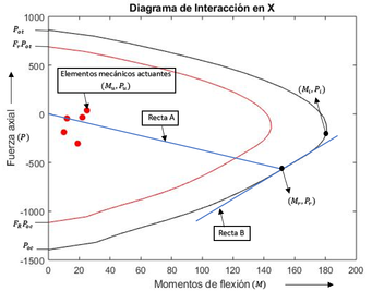
For a single variable of width for the ISR a general function to evaluate the efficiency must be established, by referring to [12] such efficiency is determined for any depth value of the neutral axis by computing an Interaction Diagram for both axis directions of a cross section geometry (if a rectangular cross section geometry is taken) Fig. 9, and then to estimate reduced with the Resistance Reduction Factor from the ACI code [1] for every flexure-compression load condition to determine their respective efficiency using Analytical Geometry (using the line intersection formula). This way a most critical condition can be determined for each iteration to take as reference of evaluation as the width of the ISR changes (decreases or increases). In structural engineering it is a common requirement for this such structural efficiency to take values between 85% to 100%
|
| Figure 9: Reference system for the determination of structural efficiency of a any flexure compression condition |
This way, an efficiency function of subjected to a constraint might be expressed as 1:
|
|
(1) |
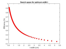
Such function for a single variable of a width value shows the following behaviour Fig. 10, presenting a non-linearity for the variation of structural efficiency as changes, forming a concave graph, with the horizontal axis corresponding to could go on until the ISR would become a solid rectangular steel profile obtaining very little non-negative values of structural efficiency, which is not practical at all, given that the resulting reinforcing bars transformed out of this steel area would not fit into the column.
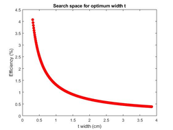
|
| Figure 10: Behaviour of the Efficiency function of a single width value (t) of the ISR |
When computing this such Efficiency function, a mathematical approach might be formulated as in [12] Fig. 11 where for rectangular solid cross section geometries quite good amount of computation might be saved than when a discrete analysis of the Idealized Steel Reinforcement is done, as formulated also by [12] for circular cross sections Fig. 12.
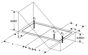
|
| Figure 11: Mathematical formulation fo the ISR method. Ideal for computational saving applied to rectangular cross-sections |
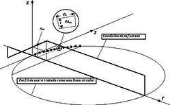
|
| Figure 12: Discrete formulation for the ISR method for circular cross-sections. Ideal for complex geometries. |
This formulation of a single variable of width for the ISR is useful as stated previously when a design based merely on codes and normative takes place, maintaining uniformity of reinforcement over the cross-section regarding a homogeneous type of reinforcing bars for each element. When a more accurate design is required, then as stated by Aschheim et. al. [9] a non-uniformity consideration might be best to carry on in order to obtain different reinforcement area for each face of the rectangular cross-section and converge better towards a minimum required total reinforcement area.
For this work and specifically for this particular case of a single variable width of the ISR the mathematical formulation for rectangular cross-sections for the efficiency function was used and performed through Multiple Linear Regression and a Gradient Descent method. The objective of the Multiple Linear Regression formulations is to get a formula so that for each structural model at hand an initial value close enough to the required one may be determined and minimize the Simple search optimization iterations. To do so, different experimental computational runs were performed varying the values of each of the variables involved in the analysis, such as and (corresponding to the section dimensions), and . As for the Gradient Descent Method, given the particular concave form of the graph function for , it could be well adapted to obtain for each structural model a value of for which the derivative of the convcave function would be less than a preestablished one Fig. 13. This way, really good approximations to the optimum cuold be gotten. The Bresler formula (2) [10] was used with the respective conditions and typical values of :
|
|
(2) |
In order to be able to apply (2) the following condition has to be satisfied to evaluate the axial loads against the design axial resistance:
Multiple Linear Regression:
Regarding the experimental runs to apply Multiple Linear Regression to estimate an initial value of , three different experimentations were performed, one with a total of 100 runs randomly registered with different values for each of the main variables involved already mentioned. The following coefficients were obtained for each interpolation method:
|
|
(3) |
Which enhances not really good approximations for initial values of to start iterating when applying a 1t-ISR, only for certain parameter values, given the linearity of the formulation as well as the high number of variables involved. The summary of the experimentation is presented in detail in the results section 4.3 for ten structural models.
Although this Multiple Linear Regression formula of may be used altogether with a Gradient Descent Optimization Method to minimize even more the number of iteration needed for a good approximation of structural efficiency wanted, as is following presented.
Steepest Gradient Descent method
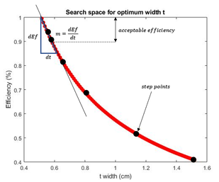
|
| Figure 13: Slope criteria for the Steepest Descent Optimization Method formulation. |
In order to obtain a range of critical slopes for the program to converge to, a total of 10 experimental models were analysed for optimization with Simple search to get to a width optimal for each model and extract its respective optimal slope. A slope range was found to be , for efficiencies between . Therefore, the middle slope () might be taken as a good algorithmic criteria for the Steepest Descent Method to converge to, although an structural efficiency range may also be used as such a criteria. The general algorithm of the program is next presented in pseudo-code.
|
| for Nmodels=1:nm |
| Compute |
| While or |
| Compute |
| Compute search direction : |
| if |
| else if |
| End if |
| Update the current |
| Compute |
| k=k+1; |
| End While |
| End for |
| FIN
|
|
Algorithm. 1 General algorithmic process for the Steepest Descent Optimization Method formulation |
One must be careful with the initial step length (it is recommended to use to avoid high number of iterations) as the step length for this case gets smaller the as it converges.
3.1.2 Multiple variables of width t values of the ISR
Regarding meta-heuristic and evolutionary algorithms there has been relevant research for the design of reinforcing steel in cocnrete structures such as [14] in which a formulation with the GA was performed, focusing primarily on costs, restricting the structural efficiencies to a pre-established range using the ISR method with a single variable to obtain an initial steel reinforcement area as minimum to generate the reinforcing bar sets taken as individuals for the algorithm. The results of this such work are good, but not that different and better than in previous work [12] in which an optimization with Simple search was carried on considering homogeneity for the type of reinforcing bar over the column; not that different neither in cost nor in efficiency, stressing the importance first of all of improve the accuracy on the required minimum reinforcing area and its distribution over the section to minimize iterations until an optimum is found through a Genetic Algorithm particularly, and secondly the need to focus specifically in structural efficiency through a complex non-uniform arrangement of reinforcing bars to obtain better solutions.
As following a comparison in performance and formulation between the GA and PSO adapted to the ISR method for two and four width variables will be carried on in order to simplify the optimization formulation for the problem through meta-heuristics given that such analysis with classical optimization would not be that practical for the reasons stressed previously, and neither through Polynomial Interpolations or Multiple Linear Regression due to the vast quantity of required data to collect in order to obtain good approximations of each different value of widths for each face of the cross-section element.
When formulating this types of problems it is quite significant and influential the way in which the structural efficiency is analysed for each possible solution of the optimal ISR. For this case the Bresler formula (4) was also employed [10], as follows:
|
|
(4) |
In order to be able to apply (4) the following condition (3.1.2) has to be satisfied to evaluate the axial loads against the design axial resistance:
For this particular case of optimization was set given to that when evaluating the efficiency with respect of the weak axis of the cross section, the bending moment is the preponderant factor when optimizing the ISR as contrary to when a single variable problem is formulated, due to the non-uniformity of the ISR over the cross section. This way, the optimization algorithm is able to minimize as much as possible the reinforcing area or widths over the cross section faces corresponding to each axis.
Similar to the analytical geometrical procedure as for a single t formulation problem, an Interaction Diagram is computed for both axis directions of a cross section geometry in order to estimate reduced with the Resistance Reduction Factor from the ACI code [1].
3.1.3 PSO-ISR for multi width variables
The basic theory of the PSO algorithm is given in Appendix B pso. It is necessary first of all to establish the range of the search space for each particle, that is the maximum and minimum values that each width variable could take for the analysis. A very simple consideration will be stated, such that the maximum reinforcement area on any face of the rectangular cross-section element is less than the sum of the maximum number of reinforcing bars with diameter such that the minimum separation from the code [1] is not violated. For the upper and lower face the maximum width of each idealized smeared reinforcement is given by (5).
|
|
(5) |
Where is maximum number of reinforcing bars allowed for that section face, is the width section dimension.
For the left and right cross-section faces (6):
|
|
(6) |
Whereas the minimum width for any variable might be just a very little number, for instance .
The general structure of the designed program with the PSO is as following:
- Generate an initial position and velocity for each particle (saving the total reinforcement area for each particle (i) for preference). In engineering terms, generate random initial values for each ISR width (j)
- Begin iterations; determining the best position and best performance (evaluating the structural efficiency for each particle). Save the best global position (). At this step, when evaluating the structural efficiency performance, a finite discrete element method of the ISR for each face of the cross section will be made. For this problem it was considered to be time-saving than to develop the mathematical formulation as when the width of the ISR remains constant
- Update position and velocity for each particle
|
|
(7) |
|
|
(8) |
|
|
(9) |
|
|
(10) |
In comparison with the single ISR with one variable in which only one solution for could take place complying the structural efficiency required range, when formulating a multiple variable problem an infinite set of solutions for a established required structural efficiency are possible, therefore a Multi-objective optimization formulation is required to minimize also the reinforcement steel area. When a two variable problem is formulated, something similar to a “Load Combination Reinforcement Diagram” as presented by Aschheim et. al. Fig. 3a is obtained, which is what in Computational Optimization is formally called a Pareto Optimal Set from which a “Pareto Front” is then generated [16]. In this problem to adapt the Multi-Objective Optimization problem, only an additional condition is required to be set, given that not necessarily one variable (taking for instance, or reinforcing area in other words) has to be in conflict with the structural efficiency as it is supposed in the majority of Multi-Objective Problems. Therefore the PSO algorithm rapidly adapts to the given two objective functions with no other operation really needed. It is of importance though, to stress that this such condition has to be carefully placed within the algorithm for a good convergence to a global optimum for both reinforcement area and structural efficiency.
This additional condition to evaluate the performance of a particle in the PSO algorithm is most recommended based on our results to be placed both when determining the best position (reinforcement area) in the current swarm and a global best position; given that a global minimum reinforcing area is preponderant to seek rather than a maximum structural efficiency (in the scale of ) as long as the structural critical efficiency requirement is covered. In fact, this structural efficiency requirement was set in the first place to minimize the reinforcement area, given that it was assumed that the less the reinforcement area is used the less efficient the structural element is.
The general algorithm for this process is resumed as following in pseudo-code. A nested PSO algorithm was generated to best estimate a global optimum reinforcement area, substituting for each iteration of the PSO the best position so far found in the previous iterations into the current run (adding such optimal position into the initial generated positions of each particle at the beginning of the PSO), thus enhancing an optimization process over that given best position to accelerate in a way the optimal results.
|
| Generate a |
| for i=1:numberPSOiterations |
| PSO-algorithm |
| Initial positions and velocities (the previous best position-) is introduced |
| for j=1:numberOptimIterations |
| Update of positions and velocities |
| endfor |
| End PSO-algorithm |
| Extract a best new t-values (new best position) |
| End for |
| globalBest-tvalues= |
| FIN
|
|
Algorithm. 2 General algorithmic process for the nested PSO-ISR |
(1) The term “Simple search” here refers to an iteration process where the step length remains constant
4 Results and discussion
4.1 Results from the application of the PSO-ISR formulation
Good results were obtained for the 4t-PSO-ISR algorithm as following presented for the given parameter values:
Structural parameters:
PSO parameters
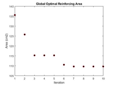
The evolution of the reinforcing along the iterations is as follows:
|
| Figure 14: Progression of reinforcing area for each iteration of the PSO-ISR algorithm |
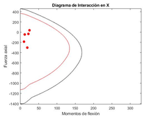
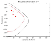
With a global optimum reinforcing area of , , .
Generating the following interaction diagrams:
|
| Figure 15: Interaction diagram in the X-axis direction for the global optima 4t-ISR |
|
| Figure 16: Interaction diagram in the Y-axis direction for the global optima 4t-ISR |
It is of relevance to stress that it takes considerable time (depending on the graphics wanted and the PSO algorithm parameters) to get to a good approximation of the global optima reinforcing area. MatLab 2017b software was used for this research, therefore the execution time may be reduced with parallel computing in another faster programming language, more likely when a higher number of structural elements are to be analysed. In any case, the results obtained are much better than with the application of a 1t-ISR Steepest Gradient Descent formulation regarding the resulting optimum area as it will be compared next.
4.2 Results from the GA-ISR formulation
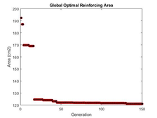
The Genetic Algorithm is also a viable option, although an little higher amount of computational execution time is necessary. Very similar results were obtained compared to the PSO algorithm. A computational experiment was also carried on with the GA and the results were as following presented with the same structural parameters and the next GA parameters.
|
| Figure 17: Evolution of the optimal reinforcing area with the GA-ISR |
With ,, and the following interaction diagrams:
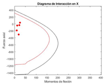
|
| Figure 18: Interaction diagram in the X-axis direction for the global optima 4t-ISR-GA |
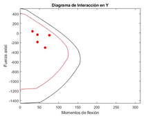
|
| Figure 19: Interaction diagram in the Y-axis direction for the global optima 4t-ISR-GA |
As it may be observed from the previous graphics obtained with the GA-ISR, it takes almost 50 generations or iterations to reach a very similar result from the PSO-ISR formulation, although still a little higher area. This results may vary from a structural model to another, and even from run to run. The mutation probability is of great influence in the final results. A further comparison between these two formulations is made in detail in further sections, as well as a general comparison between all of the formulations here presented for the ISR.
4.3 Results from the 1t ISR formulation with Multiple Linear Regression
Ten experimental random structural models were tested to register the number of iterations it would take for each to reach a wanted structural efficiency range given an initial width value previously estimated with the results from the application of Multiple Linear Regression formulation. The results are following presented:
| Point | b | h | |||||||||
| 1 | 67.857 | 185.7708 | 146.0661 | 393 | 0.89 | 4.5 | |||||
| 2 | 93 | 67 | -647.700 | 27.3106 | 144.2455 | 164 | 0.89 | 3.5 | |||
| 3 | 228 | 34 | -427.914 | 180.9444 | 121.9733 | 470 | 0.89 | 4.0 | |||
| 4 | 75 | 198 | -273.442 | 190.3260 | 184.0664 | 131 | 0.83 | 3.9 | 2.60 | ||
| 5 | 177 | 35 | -636.092 | 38.0866 | 73.7833 | 376 | 0.94 | 4.7 | |||
| 6 | 93 | 412 | 75.236 | 85.0518 | 62.5437 | 196 | 0.80 | 4.1 | 47.8 | ||
| 7 | 109 | 53 | -619.890 | 81.5238 | 163.9962 | 531 | 0.97 | 4.0 | 3.35 | 74.7 | |
| 8 | 98 | 93 | -479.857 | 91.4848 | 175.0743 | 410 | 0.88 | 3.8 | 2.74 | 91.7 | |
| 9 | 53 | 172 | -610.107 | 95.8926 | 127.8633 | 426 | 0.89 | 4.8 | 3.6 | 90.0 | |
| 10 | 58 | 73 | -444.694 | 37.9420 | 99.0011 | 188 | 0.80 | 4.3 | 4.40 |
As shown in the table, the error in most cases is even higher than . Only two initial estimations were close to the final value of which makes the method no so quite efficient for this case. It is relevant to stress that, even though the estimation with the Multiple Linear Regression may diverge, still would take much less time to get to the optimum value of from that estimation than with the application of the PSO-4t-ISR or GA-4t-ISR, although, clearly not with less reinforcement area by any means, as it would be compared further in this text.
4.4 Results from the 1t ISR formulation with the Steepest Gradient Descent method
The same ten structural models studied for the formulation of the Multiple Linear Regression method were again taken to register the maximum number of iterations it would take for the Steepest Gradient Descent Method to converge.
| Point | b | h | ||||||||
| 1 | 67.857 | 185.7708 | 146.0661 | 393 | 0.92 | 4.5 | ||||
| 2 | 93 | 67 | -647.700 | 27.3106 | 144.2455 | 164 | 0.91 | 3.5 | ||
| 3 | 228 | 34 | -427.914 | 180.9444 | 121.9733 | 470 | 0.94 | 4.0 | ||
| 4 | 75 | 198 | -273.442 | 190.3260 | 184.0664 | 131 | 0.93 | 3.9 | ||
| 5 | 177 | 35 | -636.092 | 38.0866 | 73.7833 | 376 | 0.9 | 4.7 | ||
| 6 | 93 | 412 | 75.236 | 85.0518 | 62.5437 | 196 | 0.91 | 4.1 | 16 | |
| 7 | 109 | 53 | -619.890 | 81.5238 | 163.9962 | 531 | 0.94 | 4.0 | 11 | |
| 8 | 98 | 93 | -479.857 | 91.4848 | 175.0743 | 410 | 0.96 | 3.8 | 16 | |
| 9 | 53 | 172 | -610.107 | 95.8926 | 127.8633 | 426 | 0.91 | 4.8 | 22 | |
| 10 | 58 | 73 | -444.694 | 37.9420 | 99.0011 | 188 | 0.90 | 4.3 |
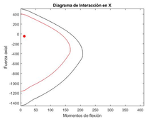
As for the same structural model taken in the PSO-ISR and GA-ISR results, the following convergence for this Steepest Gradient Descent method was found:
Structural parameters:
|
| Figure 20: Convergence of the Steepest Gradient Descent method for the 1t-ISR |
|
| Figure 21: Interaction diagram in the X-axis direction for the global optima 4t-ISR-GA |
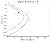
|
| Figure 22: Interaction diagram in the X-axis direction for the global optima 4t-ISR-GA |
Yielding a total reinforcing area equal to , very similar to the one obtained with the GA-ISR, not so much for the PSO-ISR which yields
4.5 Comparisons between the different ISR optimization formulations
As mentioned before, the performance of the GA depends a great deal on the mutation probability parameter. In order to see the effects of such parameter on the final results a total of five experimentation runs were done, based on the same structural model used previously with , changing the mutation probability from to for 100 generations. The summary of the relevant results are presented in the next table.
| Run | |||
| 1 | 0.015 | 97.73 | |
| 2 | 0.02 | 99.9 | |
| 3 | 0.025 | 99.87 | |
| 4 | 0.03 | 99.63 | |
| 5 | 0.035 | 99.73 | |
| 6 | 0.04 | 99.85 |
From the results above it can been observed that the more the minimum area is found for a higher value of the mutation probability, thus, it is recommended to use for faster and better convergence.
As for the PSO-ISR formulation, it is of interest to see its efficiency of convergence for different values for the parameter mainly, higher than 10, as it was experimented previously. The following table presents the results obtained for 5 experimentation with the same structural model .
| Run | |||
| 1 | 10 | 95.97 | |
| 2 | 15 | 95.98 | |
| 3 | 20 | 94.66 | |
| 4 | 25 | 97.33 | |
| 5 | 30 | 99.04 |
It is clear to see that the more the total of iterations for the PSO-ISR nested formulation, the lower the reinforcing areas, but with a much higher computational time. It could be observed from the table above that the difference between the resulting reinforcing area with 10 iterations is not really significant compared with the resultant one with 30 iterations (3 times more computational power and only a few square centimetres). It would be recommended to take 20 iterations with quite good results (much better than with the GA-ISR).
4.5.1 Additional commentaries and further research
The following step once the an optimal reinforcing area with the ISR has been obtained is to transform such area to steel bars. There might be different ways to do that, either using another optimization algorithm to optimize topologically the arrangement, position and diameter of each bar over the cross section of an element along each face or simply considering a homogeneous distribution of bars with only one diameter along each cross section face, as it would be more practical. In [14] for instance, the GA was used to optimize topologically the reinforcing steel bars once the 1t-ISR method had been used with acceptable results, but regarding a 4t-ISR method, given that a whole optimization procedure formulation has already been carried on, it would suffice to pass from this reinforcing area for each face of the cross section to a homogeneous distribution of reinforcing bars Fig. 23 minimizing thereafter the construction costs even in a greater deal.
Although the number of possible combinations of reinforcing bars could still be high ( to be precise), it would surely take less time to find a good optimum arrangement of reinforcing bars than employing a whole topological optimization as done by [14]. This way of reinforced concrete optimization could be a good matter of further research with its application on 3D concrete frames to better appreciate its advantages.

|
| Figure 23: Transformation from the 4t-ISR formulation to reinforcing bars. |
5 Conclusions
The different formulations for the ISR developed happen to be very simple to code for anyone having basic understanding of optimization methods. The time required is evidently higher for the meta-heuristic optimization formulations, rather than for the Steepest Gradient Descent method which would be the one more likely to adopt for common structural design of concrete structures, given that despite of its simplicity of formulation the results it evokes are quite acceptable. On the other hand for the application of meta-heuristics for this method, could be of greater impact is huge structural systems, being able to reduce its required execution time by adapting them to Multi-Objective optimization procedures taking on account at the same time different structural features of a structural system, such as displacements, ductility of certain elements, costs or section dimensions.
In any case, the global application fo this method, ant its official recognition in structural engineering could enhance great advantages in the way concrete structures are designed.
BIBLIOGRAPHY
[1] Building Requirements for structural concrete and commentary, American Concrete Institute ACI 318, 2019
[2] Whitney CS. Cohen E., ``Guide for ultimate strength design of reinforced concrete. ACI J, 1956; 28(5):445-90. [Proceedings V.53].
[3] Au FTK, Bai ZZ, Effect of axial load on flexural behaviour of cyclically loaded RC columns. Comput Concr 2006: 2(4):261-84
[4] Walther R. Miehlbardt M., Dimensionnement des structures en Béton. Lausanne: Press Polytechniques et Universitaires Romandes; 1990
[5] Hernánde Montes, Gil-Martin LM, Aschheim M., “The design of concrete members subjected to uniaxial bending and compression using reinforcement sizing diagrams”, ACI Struct J 2005;102(1):150-8
[6] Hernández Montes E, Gil-Martín LM, Pasadas-Fernández M, Aschheim M., “Theorem of optimal reinforcement for reinforced concrete cross sections”, Struct Multidiscip Optim 2008;36(5):509–21.
[7] Ho Jung Lee, Mark Aschheim, Hernández Montes E, Gil-Martín LM, Pasadas-Fernández M, “Optimum RC column reinforcement considering multiple load combinations”, Struct Multidiscip Optim 2009;39;153-170.
[8] L. M. Gil-Martín, E. Hdez-Montes, M. Aschheim, “Optimal reinforcement of RC columns for biaxial bending”, Materials and Structures Journal (2010), 43:1245-1256
[9] Aschheim M, Hernández-Montes E, Gil-Martín LM (2008), “Design of optimally reinforced RC beam, column and wall sections”, J Struct Eng 134(2):169–188
[10] Bresler B., Design criteria for reinforced columns under axial load and biaxial bending, ACI Proc 57:481–490
[11] Gouwens AJ (1975), Biaxial bending simplified, reinforced concrete columns, ACI Special Publication SP-50. American Concrete Institute, Detroit
[12] Luis F. Verduzco, A. Hernández, “Optimization of reinforcing steel for the design of concrete columns”, University of Guanajuato, Bachelor Thesis to obtain the grade of Civil Engineer, Mexico, 2019
[13] Gaceta Oficial de la Ciudad de México, Normas técnicas complementarias de la Ciudad de México, 2017, Normas Técnicas Complementarias para Diseño y Construcción de Estructuras de Concreto 2017
[14] Luis F. Verduzco, “Optimization of reinforcing steel with genetic algorithms for the design of concrete columns”, 14th Research Colloquium, Autonomous University of Queretaro, Mexico, 2020
[15] M. Afzal, Y. Liu, Jack C.P.Cheng, V. J.L. Gan, “Reinforced concrete structural design optimization: A critical review”, Journal of Cleaner Production-Elsevier, 2020
[16] A. Zhou, Bo-Yang Qu, Hui Li, Shi-Zheng Zhao, P. Nagaratnam, Q. Zhang, “Multiobjective evolutionary algorithms: A survey of the state of the art”, Journal of Swarm and Evolutionary Computation, doi:10.1016/j.swevo.2011.03.001
Document information
Published on 07/01/21
Submitted on 07/01/21
Volume 5, 2021
Licence: CC BY-NC-SA license
Share this document
Keywords
claim authorship
Are you one of the authors of this document?