Bearing life prediction based on critical interface method under multiaxial random loading

Revision as of 13:34, 27 April 2023

Abstract

The bearing was a key component of the mining machine tire unloader machine and was subjected to random multiaxial stress during operation. Therefore, the life prediction of bearing was of safety guidance. In this paper, a bearing life prediction method based on the critical plane method under multiaxial random loading was proposed. Firstly, a virtual prototype model was built based on the actual working conditions of the tire unloader machine to obtain the time load history of the bearing. Transient dynamic analysis of the bearing was carried out to obtain the triaxial stress-strain time histories at the hazardous locations of the bearing. A new coordinate system was established using the hazard node as the coordinate origin, and the location of the critical plane was searched for based on the critical plane multiaxial fatigue theory, combined with the maximum shear strain amplitude on the critical plane for multi-axial rain flow cycle counting to obtain the damage amount in each direction. At the same time, the life calculated from the maximum damage amount was used as the final life, resulting in a cycle count of the bearing of 268,303 cycles and a duration of 1490.58h. The results of this study could be used as a guide to predict the service life of the bearing in large machinery subjected to multiaxial random stress conditions.

Keywords: Multiaxial random loading, dynamic simulation, critical plane method, life prediction

1. Introduction

While the machinery industry is gradually developing, rolling bearings are widely used in complex rotating machines and systems such as motors, ships and robots. The rolling bearing is one of the most widely used components in modern machinery, which relies on rolling contact between the main elements to support the rotating parts. According to statistics, around 30% of rotating machinery failures are caused by rolling bearing failures. Therefore, condition monitoring and life prediction of the rolling bearing is essential for the proper functioning of rotating machinery.

The rolling bearing is the core component of a giant mining tire unloader machine, which is often subjected to complex multi-axial cyclic loads during service. This poses a serious challenge for the accurate prediction of fatigue life. As production progresses and time accumulates, the bearing's performance and health status will weaken under the action of multiaxial stress. If computer simulations are used to simulate the actual loading of the bearing before it enters service, multiaxial fatigue life prediction can be carried out on the bearing before it becomes dangerous to replace it to ensure the production schedule of the company as well as to prevent the safety of the company's personnel and property from being endangered.

Bearing life is an important indicator of the performance of a rolling bearing. The bearing fatigue life prediction models can be categorized into engineering models, traditional statistical life prediction models and state detection-based data prediction models according to the characteristics and applications of rolling bearing life. driven models. Engineering models include the Lundberg-Palmgren (L-P) model [1], the Ioannides-Harris (I-H) model [2] and the Zaretsky model [3]. In 1947, Lundberg and Palmgren [1] proposed the L-P theory based on the subsurface orthogonal tangential stress and combined it with the Weibull distribution function, which became the basis of rolling bearing life prediction. At this stage, scholars have modified the traditional L-P theory formulation according to practical needs. Yakout et al. [4] used the modal experimental method to find out the frequency response function graphs of four different bears, solved the dynamic characteristics of the bearing (natural frequency and modal vibration pattern) by the first vibration mode, and solved the actual equivalent dynamic load of the bearing by the dynamic characteristics. The fatigue life of the bearing was then solved by parameter revision according to the L-P theory. Gupta et al. [5] compared the L-P model with the Zaretsky model and the Zaresky model predicted a higher bearing life at lower loads. As the load increased the Zaresky model's sensitivity to load resulted in a dramatic decrease in the predicted life. Klebanov et al. [6] modified the L-P model and the Zaretsky model based on the concept of dynamic stress capacity, using 32220bearing as an example. Comparing the stability results of the shear stress life index of the two models showed that the improved L-P model had higher validity characteristics. Cheenady et al. [7] proposed a new perspective on the use of plastic stress fields in bearing life prediction compared to the traditional L-P, I-H and Zaretsky models, and introduced two probabilistic models based on the Dang Van criterion to compare with the traditional models applying elastic stress fields. The results show that the bearing life prediction considering the plastic stress field is more accurate. Lei et al. [8] developed a bearing residual use life prediction method based on a stochastic process model and demonstrated the accuracy of the method by simulating the degradation process and accelerated degradation tests using bearing. One disadvantage of using both engineering-based models and traditional statistical life prediction models is that the selection of equation parameters greatly affects the accuracy of life prediction results. At the same time, due to the development of intelligent bearings, it is not necessary to determine the parameters needed for the engineering model, but rather to directly signal the vibration of the bearing by means of sensors. As a result, a number of data-driven bearing life prediction models based on state detection have emerged. Depending on the class of signals collected by the sensors, the data-driven approach is divided into a bearing degradation phase and a bearing using life prediction phase [9]. Many scholars have done in-depth research on data-driven methods [10-12]. For example, Cao et al. [13] used interval whitening methods to reduce the disturbance from non-smooth runs, constructed a remaining lifetime model for bearing by Gaussian process algorithm and compared it with support vector regression methods and artificial neural network methods. The prediction accuracy of the method was improved by more than 65.8%. Gao et al. [14] established a new health index and bearing degradation state model by extracting the time domain features of bearing vibration signals. Wu et al. [15] used the algorithm called vanilla LSTM neural network to obtain more accurate bearing life prediction results compared to traditional RNN and GRU in complex operating conditions. However, the data-driven bearing life prediction model also has disadvantages, such as errors in the data collection process, improper handling and uncertainties in the nature of the bearing material. At the same time, there are shortcomings in the experimental conditions themselves. Due to the complexity of the bearing practical application process and the limitations on data transfer and storage, it is not possible to carry out effective data acquisition of the bearing vibration process.

Bearing fatigue damage mostly occurs in the multiaxial stress state, and most critical structural components in major equipment in service in aerospace, transportation and robotics are subjected to complex multi-axial loads, and the accuracy of their life prediction affects the detection and safety of critical equipment in service [16-20]. There are three methods for multiaxial fatigue analysis: the equivalent effect variation method [21-24], the energy method [25-29] and the critical interface method [30-34]. The equivariance method is simple and only applies the uniaxial tension-compression fatigue model to the prediction of multiaxial fatigue life, and the relationship between equivariance and life lacks a physical basis, as it does not take into account the influence of the loading path and the additional strengthening of the material during the stress cycle. As a result, the prediction accuracy of the equivalent effect method under non-proportional loading conditions is low. The energy method was first proposed by Feltner and Morrow [35] in 1961, who argued that with each cycle of stress cycling, a plastic work is accumulated, which leads to irreversible damage to the part and ultimately to fatigue failure. The accumulation of plastic work leads to irreversible damage of the part and ultimately to fatigue failure. The critical interface method was developed by Brown and Miller [36] in 1973, after extensive fatigue life experiments, when they concluded that two stress-strain parameters were required for multiaxial fatigue life prediction of parts. critical interface method. The key to the critical interface method is to determine the location of the critical plane and to record the damage parameters at the critical plane for fatigue life prediction by selecting the corresponding intrinsic structure model.

In this thesis, a 61918 deep groove ball bearing on a giant mining tire unloading machine is studied as a concrete example. In this paper, a virtual prototype model of the bearing is developed to simulate the actual operating conditions of the bearing and to collect the time load history of the bearing in the absence of vibration signal measurement equipment. Then, the stress and strain histories at the hazardous locations of the bearing are identified through transient dynamic simulation, and the coordinate system is established using this point as the origin of the coordinates, and the plane of maximum shear strain with maximum positive strain is used as the criterion for the critical plane search. The Wang-Brown cycle counting method is used to predict the critical plane orientation and fatigue life of the bearing based on complex multi-axial loading situations.

2. Multiaxial fatigue life prediction model based on critical plane method

This section begins with a review of the method for determining the critical plane. The first step is to determine the dangerous part of the bearing as the fatigue initiation point based on the load time history of the bearing under actual operating conditions. Next, the exact location of the critical plane and the stress-strain history on its face is determined by combining the critical plane method with the weight function method. It is then counted by the multi-axis rain flow counting method. The damage of a single cycle of bearing is predicted by combining the Manson-Coffin equation, and finally the damage is accumulated according to the damage accumulation criterion to complete the life prediction.

2.1 General stress-strain state of arbitrary plane

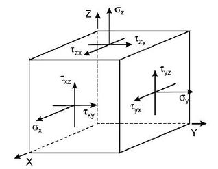
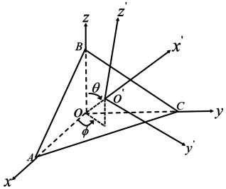
According to elastodynamics, the general stress state of the micro-element is divided into six stress components ${\textstyle {\sigma }_{x}}$ , ${\textstyle {\sigma }_{y}}$ , ${\textstyle {\sigma }_{z}}$ , ${\textstyle {\tau }_{xy}}$ , ${\textstyle {\tau }_{xz}}$ , ${\textstyle {\tau }_{yz}}$ , as shown in Figure 1. Determining the critical plane begins by comparing the magnitude of the general stress-strain in an arbitrary plane, which is generally obtained by rotation of the standard Cartesian coordinates. The principle of coordinate rotation is to first determine that the new coordinate axis is perpendicular to the currently determined plane and that the other two coordinate axes are parallel to the determined plane, as shown in Figure 2. ${\textstyle xoy}$ is assumed to be the free surface of the material and ABC is the new plane, perpendicular to ${\textstyle ABC}$ , where ${\textstyle \phi }$ is the angle between the projection of ${\textstyle x{}'}$ in the ${\textstyle xoy}$ plane and ${\textstyle x}$ . ${\textstyle \theta }$ is the angle between the ${\textstyle x{}'}$ and ${\textstyle z}$ axes. The transformation between the new coordinates and the original coordinates can be expressed as the directional cosine about ${\textstyle \phi }$ and ${\textstyle \theta }$ . The directional cosines of the new coordinates to the original coordinate system are shown in the Table 1.


Figure 1. Stress component in the general state


Figure 2. Stress in an arbitrary plane

Table 1. Cosine of the direction between the new and original coordinates

	${\textstyle X}$	${\textstyle Y}$	${\textstyle Z}$
${\textstyle X{}'}$	${\textstyle a_{11}}$	${\textstyle a_{12}}$	${\textstyle a_{13}}$
${\textstyle Y{}'}$	${\textstyle a_{21}}$	${\textstyle a_{22}}$	${\textstyle a_{23}}$
${\textstyle Z{}'}$	${\textstyle a_{31}}$	${\textstyle a_{32}}$	${\textstyle a_{33}}$

Of which:

\left[{\begin{array}{ccc}a_{11}&a_{12}&a_{13}\\a_{21}&a_{22}&a_{23}\\a_{31}&a_{32}&a_{33}\end{array}}\right]=\left[{\begin{array}{ccc}\cos \phi \sin \theta &\sin \phi \sin \theta &\cos \theta \\-\sin \theta &\cos \phi &0\\-\cos \phi \cos \theta &-\sin \phi \cos \theta &\sin \theta \end{array}}\right]

(1)

The relationship between the stresses in the new coordinate system and the transformation of the stresses in the original coordinate system can be expressed as follows:

\left[{\begin{matrix}{{\sigma }_{x'}}\\{{\sigma }_{y'}}\\{{\sigma }_{z'}}\\{{\tau }_{x'y'}}\\{{\tau }_{x'z'}}\\{{\tau }_{y'z'}}\\\end{matrix}}\right]=

\left[{\begin{matrix}a_{11}^{2}&a_{12}^{2}&a_{13}^{2}&2{{a}_{11}}{{a}_{12}}&2{{a}_{11}}{{a}_{13}}&2{{a}_{13}}{{a}_{12}}\\a_{21}^{2}&a_{22}^{2}&a_{23}^{2}&2{{a}_{21}}{{a}_{22}}&2{{a}_{21}}{{a}_{23}}&2{{a}_{23}}{{a}_{22}}\\a_{31}^{2}&a_{32}^{2}&a_{33}^{2}&2{{a}_{31}}{{a}_{32}}&2{{a}_{31}}{{a}_{33}}&2{{a}_{33}}{{a}_{32}}\\{{a}_{11}}{{a}_{21}}&{{a}_{12}}{{a}_{22}}&{{a}_{13}}{{a}_{23}}&({{a}_{11}}{{a}_{22}}+{{a}_{12}}{{a}_{21}})&({{a}_{13}}{{a}_{21}}+{{a}_{11}}{{a}_{23}})&({{a}_{12}}{{a}_{23}}+{{a}_{13}}{{a}_{22}})\\{{a}_{11}}{{a}_{31}}&{{a}_{12}}{{a}_{32}}&{{a}_{13}}{{a}_{33}}&({{a}_{11}}{{a}_{32}}+{{a}_{12}}{{a}_{31}})&({{a}_{13}}{{a}_{31}}+{{a}_{11}}{{a}_{33}})&({{a}_{13}}{{a}_{32}}+{{a}_{12}}{{a}_{33}})\\{{a}_{21}}{{a}_{31}}&{{a}_{22}}a{}_{32}&{{a}_{23}}{{a}_{33}}&({{a}_{21}}{{a}_{32}}+{{a}_{22}}{{a}_{31}})&({{a}_{23}}{{a}_{31}}+{{a}_{21}}{{a}_{33}})&({{a}_{22}}{{a}_{33}}+{{a}_{23}}{{a}_{32}})\end{matrix}}\right]

(2)

As with the stress state, the general strain state of a tiny unitary body is divided into six components, ${\textstyle {\epsilon }_{x}}$ , ${\textstyle {\epsilon }_{y}}$ , ${\textstyle {\epsilon }_{z}}$ , ${\textstyle {\gamma }_{xy}}$ , ${\textstyle {\gamma }_{xz}}$ , ${\textstyle {\gamma }_{yz}}$ . The strain state in either plane is obtained by rotating the co-ordinate system in the same principle as the stress state, using the directional cosine of ${\textstyle \phi }$ and ${\textstyle \theta }$ to represent it. The strain in the new c-ordinate system can be expressed as follows in relation to the strain transformation in the original c-ordinate system

\left[{\begin{array}{c}{\begin{array}{c}{\epsilon }_{x'}\\{\epsilon }_{y'}\\{\epsilon }_{z'}\end{array}}\\{\frac {{\gamma }_{x'y'}}{2}}\\{\frac {{\gamma }_{x'z'}}{2}}\\{\frac {{\gamma }_{y'z'}}{2}}\end{array}}\right]=

\left[{\begin{array}{cccc}{\begin{array}{ccc}{\begin{array}{c}{\begin{array}{c}a_{11}^{2}\\a_{21}^{2}\\a_{31}^{2}\end{array}}\\a_{11}a_{21}\\a_{11}a_{31}\\a_{21}a_{31}\end{array}}&{\begin{array}{c}{\begin{array}{c}a_{12}^{2}\\a_{22}^{2}\\a_{32}^{2}\end{array}}\\a_{12}a_{22}\\a_{12}a_{32}\\a_{22}a_{32}\end{array}}&{\begin{array}{c}{\begin{array}{c}a_{13}^{2}\\a_{23}^{2}\\a_{33}^{2}\end{array}}\\a_{13}a_{23}\\a_{13}a_{33}\\a_{23}a_{33}\end{array}}\end{array}}&{\begin{array}{c}{\begin{array}{c}2a_{11}a_{12}\\2a_{21}a_{22}\\2a_{31}a_{32}\end{array}}\\\left(a_{11}a_{22}+a_{12}a_{21}\right)\\\left(a_{11}a_{32}+a_{12}a_{31}\right)\\\left(a_{21}a_{32}+a_{22}a_{31}\right)\end{array}}&{\begin{array}{c}{\begin{array}{c}2a_{11}a_{13}\\2a_{21}a_{23}\\2a_{31}a_{33}\end{array}}\\\left(a_{13}a_{21}+a_{11}a_{23}\right)\\\left(a_{13}a_{31}+a_{11}a_{33}\right)\\\left(a_{23}a_{31}+a_{21}a_{33}\right)\end{array}}&{\begin{array}{c}{\begin{array}{c}2a_{13}a_{12}\\2a_{23}a_{22}\\2a_{33}a_{32}\end{array}}\\\left(a_{12}a_{23}+a_{13}a_{22}\right)\\\left(a_{13}a_{32}+a_{12}a_{33}\right)\\\left(a_{22}a_{33}+a_{23}a_{32}\right)\end{array}}\end{array}}\right]

\,\,\left[{\begin{array}{c}{\begin{array}{c}{\epsilon }_{x}\\{\epsilon }_{y}\\{\epsilon }_{z}\end{array}}\\{\frac {{\gamma }_{xy}}{2}}\\{\frac {{\gamma }_{xz}}{2}}\\{\frac {{\gamma }_{yz}}{2}}\end{array}}\right]

(3)

2.2 Selection of critical surfaces and damage parameters

For multiaxial fatigue damage calculations, the most widely used method is the critical surface method. The criterion for selecting the critical surface is to find the maximum shear strain plane with the maximum normal strain. For multi-axial loading time histories, the maximum shear strain plane with the maximum positive strain is found as the critical plane by varying the orientation angle, and the stress-strain history on the critical plane is calculated. Next, the stress-strain history at the critical plane is converted into a single cycle fatigue damage quantity based on a specific fatigue damage model. Finally, damage accumulation is carried out according to the damage accumulation criterion to complete the bearing life prediction.

Under random multi-axial loading conditions, it is known from the shear-strain reciprocity theorem that mutually perpendicular planes have the same maximum shear strain amplitude. Therefore, there is not a single plane within the material that has the maximum shear strain. At this point it is necessary to compare the maximum positive strain to select the critical plane, which determines the critical plane orientation angle ${\textstyle \left({\phi }_{cr},{\theta }_{cr}\right)}$ at this point in time. From the critical angle at each moment the shear strain at the critical plane at each moment can be determined, i.e. ${\textstyle {\gamma }_{max}}$ for that moment. The weights at that moment are determined by combining the Manson-Coffin equation to calculate the damage value at that moment. A weighted average of the critical angle is then calculated using the weight function method to calculate the weighted critical angle. The shear strain, positive strain and positive stress in the critical plane after weighting are determined. The equations for the maximum shear strain ${\textstyle {\gamma }_{max}}$ and the critical angle ${\textstyle \left({\phi }_{cr},{\theta }_{cr}\right)}$ are shown below:

(4)

(5)

(6)

(7)

(8)

where ${\textstyle D\left(t\right)}$ is the damage value corresponding to the critical plane at each moment, and ${\textstyle W\left(t\right)}$ is the weight value corresponding to the damage at that moment. The critical plane orientation angles at different moments are weighted and summed according to the weights to obtain the weighted critical angles ${\textstyle {\phi }_{cr}}$ and ${\textstyle {\theta }_{cr}}$ . ${\textstyle {\sigma }_{f}^{'}}$ is the fatigue strength factor and ${\textstyle {\epsilon }_{f}^{'}}$ is the fatigue ductility index. The physical significance of ${\textstyle b}$ and ${\textstyle c}$ is the fatigue strength index and the fatigue ductility index, as well as ${\textstyle N_{k}}$ is the value of life under uniaxial fatigue. The weight function is used to characterize the contribution of the potential angle of the maximum normal strain with the maximum shear strain amplitude at each moment to the potential angle of the critical plane for the entire load history. The critical plane for the entire load history is obtained by ${\textstyle t_{N}}$ -weighted averaging of planes of maximum normal positive strain with the same maximum shear strain amplitude.

The multiaxial fatigue damage model used in this paper is the Wang-Brown model. The Wang-Brown model takes into account the additional strengthening effect due to the rotation of the plane where the maximum shear strain is located, and introduces positive stresses and strains in the plane where the maximum shear strain is located in the parameter control. The expressions of the model are as follows:

(9)

(10)

where ${\textstyle \Delta {\gamma }_{\max }/2}$ is the maximum shear strain amplitude; ${\textstyle E}$ is the bearing steel modulus of elasticity; ${\textstyle N_{f}}$ is the fatigue life; ${\textstyle {\sigma }_{n,mean}}$ is the average positive stress within the critical surface shear strain cycle; ${\textstyle {\epsilon }_{n}^{\ast }}$ is the normal positive strain variation between two adjacent maximum shear strain return points on the critical plane; ${\textstyle \upsilon }$ is the bearing steel Poisson's ratio. The multi-axial parameter ${\textstyle S}$ can be determined from the tensile and torsional fatigue limits as in Eqs.(4)-(11)

(11)

where ${\textstyle {\tau }_{-1}}$ and ${\textstyle {\sigma }_{-1}}$ are the torsional and tensile limits of the material. Multiaxial fatigue has the parameter values shown in the Table 2.

Table 2. Multiaxial fatigue parameter value

${\textstyle {\sigma }_{f}^{'}}$	${\textstyle {\epsilon }_{f}^{'}}$	${\textstyle b}$	${\textstyle c}$	${\textstyle S}$
2425	-0.0087	0.59	-0.58	0.8

2.3 Multiaxial cycle counting

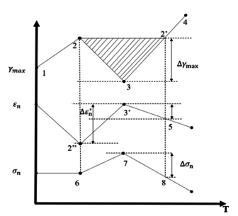
The basic idea of the multi-axis rainfall counting method is to calculate the main parameters by means of rainfall counting. The calculation of the auxiliary parameters is then completed by using the counting cycle for the primary parameter to correspond to the counting cycle for the secondary parameter. The main parameter of the critical plane is the maximum magnitude of the shear strain in the critical plane, and the number of positive stresses and positive strains within the shear strain cycle is determined by the shear strain cycle. The principle of multi-axis rainfall counting is shown in Figure 3. 2-3-2’ is a course of shear strain cycle counts, the middle point is known as the cut-off point and the cycle is picked by comparing the amplitudes by moving back from the previous point. The distance 2’-3 in the figure is the maximum shear strain amplitude. The positive strain variation and the average positive stress are also determined within the corresponding cycle.


Figure 3. Schematic diagram of a single cycle of the multi-axis rainfall counting method

3. Simulation analysis

3.1 Bearing load history acquisition

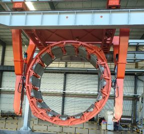
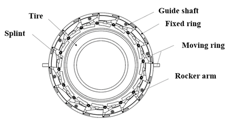
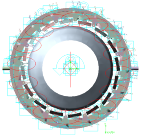
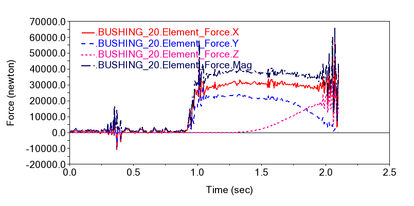
The complete machine of tire unloader machine is shown in Figure 4. Using the modelling software, a 3D model of the tire unloader machine is created and the components of the tire unloader machine are shown in the Figure 5. The 3D model of the tire unloader machine is imported into the dynamics software, and the relevant constraints and loads are added according to the actual working conditions to establish a virtual prototype model of the tire unloader system. The whole mechanism of the tire unloader machine is mainly based on the rotating sub-assemblies. The rotating sub-assemblies are applied to the hinge of the connecting rod and the rotating joints of the clamp plate and the ro'scker arm. The fixed ring is fixed to the fixed ring, and the rotating connection is applied between the guide wheel and the guide wheel shaft. The virtual prototype model of the tire unloader machine is shown in Figure 6. The tires unloaded by the giant mining tire unloader machine weigh up to 6 tonnes. After the tires have been shaped once, they need to be clamped and fixed by the unloader and turned 90° for transport, where the mechanical arm is subjected to downward inertia forces. A dynamic simulation of the tire unloader as a whole was carried out, and the three-way load history at the lowermost mechanical arm of the unloader bearing was obtained by applying constraints and loads according to the above working conditions, as shown in Figure 7. The bearing is fixed in the outer ring under working conditions and is pressed on one side, where it is subjected to axial forces in the ${\textstyle z}$ -direction, transverse forces in the ${\textstyle y}$ -direction and vertical forces in the ${\textstyle x}$ -direction. The bearing exists in pairs, so when analyzing the forces on a single bearing, the transverse and vertical forces are half of the load history and the axial force remains unchanged.


Figure 4. The physical diagram of mine tire unloader machine


Figure 5. Schematic diagram of tire unloader machine parts


Figure 6. Tire unloader machine virtual prototype model


Figure 7. Load time history of bearing under actual load

3.2 Comparative verification

In order to verify the rationality of the load time history results, the convolution neural network is used to identify the real-time output torque proportional coefficient of the tightening motor on the control panel when the tire unloader machine is running. A video camera is used to capture the readings displayed on the control panel of the tightening motor in real time at a frame rate of 30 frames/s, i.e. 30 images per second.

Digital identification of each frame in the video in turn, as the dynamic ring drive of the tire unloader machine consists of a clamping motor, a reducer, and a screw. The reducer is connected with the motor to reduce the output speed and increase the output torque. The screw is connected with the reducer to convert the rotation movement into the movement of the screw and drive the rotating ring. The image data identified is the rated output torque scale factor of the motor, which needs to be converted into the real thrust on the moving ring, i.e. the screw thrust. The output torque of the reducer is related to the motor parameters as shown in Eq.(12), where the motor power ${\textstyle P}$ is 0.75kW and the speed is ${\textstyle n=1500}$ r/min. The transmission efficiency is ${\textstyle \eta }$ is 98% and the motor to reducer speed ratio ${\textstyle r=20:1}$ , the maximum output torque ${\textstyle T_{a}}$ of the reducer is calculated to be 94N·m. The conversion equation between the output torque of the reducer and the screw thrust ${\textstyle F_{a}}$ is shown in Eq.(13), with a screw lead ${\textstyle t=10}$ mm and a conversion efficiency of 95%. The maximum thrust force ${\textstyle F_{a}}$ of the screw is calculated from the maximum output torque to be 56N. The motor torque output scaling factor is converted to the thrust variation value of the moving ring and the torque factor and actual moving ring thrust values are listed in Table 3

(12)

(13)

Table 3. Output torque scaling factor vs. actual dynamic ring thrust value (partial)

Output torque scaling factor (‰)	Actual dynamic ring thrust (N)
232	12.99
239	13.38
244	13.66
250	14.00
258	14.45
262	14.67
269	15.06
276	15.46
283	15.85
289	16.18
295	16.52
302	16.91
309	17.30
317	17.75
321	17.98
327	18.31

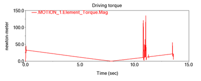
Figure 8 shows the drive torque values from the dynamic simulation.


Figure 8. Simulated dynamic ring drive torque variation curve for tire unloader machine

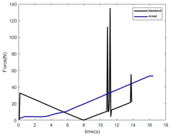
The numerical results of the simulation are the values of the torque variation of the dynamic ring drive, which is located in the centre of the unloading machine. Based on the actual radius of the unloader being approximately 1m, the value of the kinematic ring thrust is considered to be numerically equal to the value of the drive torque. The calculated variation of the actual thrust of the kinematic ring is compared with the simulated value of the kinematic ring drive of the unloader and the results are shown in Figure 9.


Figure 9. Comparison of simulated and actual values

The simulated drive of the kinematic ring is different from the actual drive. In the simulation, the rotational drive is applied directly to the moving ring, which starts from a standstill to the beginning of the movement and requires higher torque. Afterwards, the drive torque required decreases due to the inertia of the kinematic ring itself. To maintain the motion, it is then gradually increased. During this process, the collision between the moving ring and the guide wheel also causes a sudden increase in torque, resulting in a peak. In practice, the drive consists of a motor, a reducer and a screw. The reducer is connected to the motor to reduce the speed and increase the output torque, which is transformed by the screw from the output torque of the reducer into a thrust on the screw to drive the moving ring for rotation. This process allows for customized settings of motor speed, output torque magnitude etc. The torque magnitude is independent of the effect of the interaction between the mechanisms during the operation of the device. Therefore, the screw thrust tends to rise gradually and with little fluctuation. However, the simulated force values are of the same order of magnitude as the actual force values, and the overall trend is towards a gradual increase, which justifies the simulation to a certain extent.

3.3 Bearing transient dynamic analysis

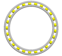
The bearing chosen for the mechanical arm is the 61918 deep groove ball bearing, the actual parameters are shown in Table 4. In the process of clamping and flipping tires, complex multi-axis cyclic loads are applied, and the normal operation of the deep groove ball bearing ensures the smooth operation of the mechanical arm of the tire unloading machine. According to the actual parameters of the bearing, a three-dimensional model of the bearing is built, omitting non-important structures such as chamfers, rounded corners and cages. The simplified 3D model is shown in Figure 10.

Table 4. 61918 bearing parameters

Symbol	Size	Meaning of the symbol
${\textstyle d}$	${\textstyle 90}$ mm	Inner diameter
${\textstyle D}$	${\textstyle 125}$ mm	Outer diameter
${\textstyle B}$	${\textstyle 18}$ mm	Width
${\textstyle d_{1}}$	${\textstyle \approx 101.4}$ mm	Inner ring shoulder diameter
${\textstyle D_{1}}$	${\textstyle \approx 113.7}$ mm	Outer ring shoulder diameter/internal seat diameter
${\textstyle r_{1,2}}$	${\textstyle min.1.1}$ mm	Outer ring chamfer size


Figure 10. 61918 bearing 3D model

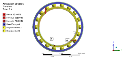
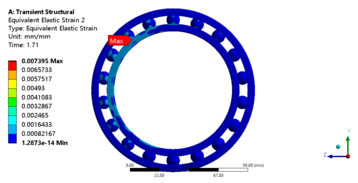
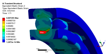
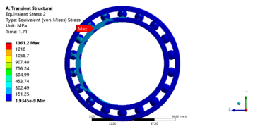
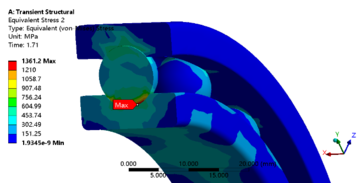
The load time history of the bearing is loaded and the bearing is restrained according to the actual working conditions. The bearing is loaded as shown in Figure 11. The bearing as a support component does not rotate during the clamping of the tire by the tire unloader and during the 90° flip. Therefore, the bearing is set to be fully fixed on the outer ring and fully constrained on the bottom surface of the inner ring, and the cage action on it is simulated by constraining the direction of rotation of the ball using the column coordinate system. The simulation time step is set to 0.005s and the results of the equivalent force and deformation of the bearing are shown in Figure 12 to Figure 15. The maximum equivalent force appears on the bearing ball, with a value of 1361.2 MPa, and the maximum equivalent effect becomes 7.40e-3 mm/mm, as well as its position is close to the maximum equivalent force. This can be assumed that the bearing ball will be the first to suffer fatigue damage.


Figure 11. Actual bearing load


Figure 12. The cloud map of equivalent strain of transient dynamics of 61918 bearing


Figure 13. The equivalent strain local cloud map of 61918 bearing ball transient dynamics


Figure 14. Equivalent stress cloud map of 61918 bearing transient dynamics


Figure 15. The equivalent strain local cloud map of 61918 bearing ball transient dynamics

4. Results and discussions

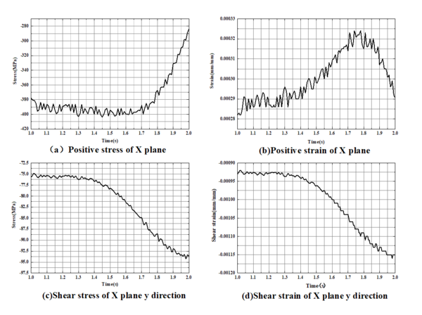
After completing the transient dynamic analysis of the bearing, the maximum point of the equivalent force is found by coupling with ANSYS. The maximum equivalent stress node number is 917. The triaxial stress strain history of node 917 is extracted and part of the stress-strain history is shown in Figure 16.


Figure 16. Stress and strain at node 917

Translate the general state of stress and strain to any plane according to Eqs.(1-3). ${\textstyle \theta }$ and ${\textstyle \phi }$ take values in the range ${\textstyle \left[0,{180}^{\circ }\right]}$ . Taking into account the calculation accuracy and calculation time, the angular step is set at ${\textstyle {10}^{\circ }}$ . The plane with the maximum positive strain variation and the maximum shear strain amplitude is the critical plane according to the angle change. A total of 64800 search results were obtained by searching ${\textstyle 18\times 18}$ faces at each moment. The strain results on different planes at any given moment are shown in the Table 5.

Table 5. Different dimensional strain values at any given moment (partial)

${\textstyle \varepsilon _{zz}}$	${\textstyle \gamma _{xz}}$	${\textstyle \gamma _{yz}}$
0	0	0
2.82E-04	1.03E-03	9.30E-04
6.62E-04	1.13E-03	-2.50E-05
1.05E-03	1.10E-03	-9.79E-04
1.41E-03	9.29E-04	-1.90E-03
1.69E-03	6.51E-04	-2.77E-03
1.86E-03	2.95E-04	-3.55E-03
1.89E-03	-9.74E-05	-4.22E-03
1.79E-03	-4.78E-04	-4.77E-03
1.56E-03	-8.00E-04	-5.17E-03
1.24E-03	-1.03E-03	-5.42E-03
8.62E-04	-1.13E-03	-5.49E-03
4.70E-04	-1.10E-03	-5.41E-03
1.13E-04	-9.29E-04	-5.15E-03
-1.65E-04	-6.51E-04	-4.75E-03
-3.32E-04	-2.95E-04	-4.19E-03
-3.67E-04	9.74E-05	-3.51E-03
-2.65E-04	4.78E-04	-2.73E-03
-4.00E-05	8.00E-04	-1.86E-03
-2.04E-04	1.95E-03	1.83E-03
5.25E-04	2.91E-04	-6.96E-04
1.15E-03	1.43E-03	-5.12E-04
1.49E-03	9.09E-04	-1.62E-03
9.55E-04	-2.75E-04	-3.17E-03

In a random multiaxial stress state, the plane in which the material has the maximum shear strain at different moments is identified according to the weighted average critical plane criterion. According to the shear strain reciprocity theorem, a pair of mutually perpendicular planes have equal maximum shear strains at the same moment. Therefore, the maximum positive strain variation is introduced as a measure, and the plane with the maximum positive strain is used as the critical plane. The plane of maximum shear strain with maximum positive strain in the material at each moment is selected as the critical plane at that moment. The results of the calculation are shown in Table 6.

Table 6. Selection of critical surfaces at different moments (partial)

${\textstyle \theta ^{\circ }}$	$\phi ^{\circ }$	$\varepsilon$ (mm/mm)	$\gamma$ (rad/rad)
100	60	-1.32E-02	1.09E-02
100	60	-1.30E-02	1.08E-02
100	60	-1.31E-02	1.09E-02
100	60	-1.33E-02	1.10E-02
100	60	-1.32E-02	1.10E-02
100	60	-1.31E-02	1.08E-02
100	60	-1.32E-02	1.09E-02
100	60	-1.33E-02	1.10E-02

As can be seen from the data in the table, because of the small time step set for the transient analysis, the changes in the stress and strain state at the danger point are small at adjacent moments and the critical plane does not produce large changes. At different moments, the plane of maximum shear strain with maximum positive strain is mainly concentrated in the ( ${\textstyle 100^{\circ },60^{\circ }}$ ) plane.

According to the Manson-Coffin equation, the maximum shear strain on the critical plane at each moment is calculated as a weight and weighted sum, and the critical plane of the weights is found to be ${\textstyle \theta =100^{\circ }}$ and $\phi =60^{\circ }$ . ${\textstyle \theta =100^{\circ }}$ and $\phi =60^{\circ }$ are chosen as the final critical plane.

According to the Wang-Brown model, the mechanical parameter for damage calculations is an equivalent effect variable $\Delta \gamma /2$ synthesised from the maximum shear strain amplitude on the critical plane and the maximum positive strain variation. Under random multiaxial stress, the direction and magnitude of the maximum shear strain varies from moment to moment. Damage calculations based on shear strains in different directions give different results. In this chapter, in order to obtain the amount of damage in the maximum damage direction, a new direction angle $\omega$ is introduced so that the direction angle $\omega$ is searched on the critical plane in steps of 10° to find the shear strain history in each direction. Combined with the positive strain and stress on the critical plane, multiaxial cycle counting is performed on the damage parameters in each direction. Finally, the multiaxial fatigue model and the cycle counting results are used to find the damage in each direction and the life calculated from the maximum damage is the final life. The results of the damage calculation in each direction, the strain history in the maximum damage direction and the results of multiaxial cycle counting in the maximum damage direction are presented in Tables 7, 8 and 9.

Table 7. Calculation results of damage in different directions

Directional angle $\omega$ (°)	Amount of damage
0	1.05E-14
10	5.15E-15
20	1.44E-15
30	3.34E-16
40	4.60E-17
50	3.06E-18
60	2.29E-23
70	2.75E-15
80	1.97E-07
90	9.23E-07
100	1.38E-06
110	1.87E-06
120	2.39E-06
130	2.89E-06
140	3.32E-06
150	3.61E-06
160	3.73E-06
170	3.65E-06

Table 8. Time course of normal positive strain, positive stress and maximum damage direction shear strain on the critical plane (partial)

${\textstyle \varepsilon }$	${\textstyle \gamma }$	${\textstyle \sigma }$
-1.28E-02	1.04E-02	-2.04E+03
-1.29E-02	1.05E-02	-2.05E+03
-1.29E-02	1.05E-02	-2.05E+03
-1.29E-02	1.05E-02	-2.05E+03
-1.30E-02	1.05E-02	-2.06E+03
-1.30E-02	1.06E-02	-2.07E+03
-1.32E-02	1.07E-02	-2.10E+03
-1.34E-02	1.09E-02	-2.13E+03
-1.34E-02	1.09E-02	-2.13E+03
-1.33E-02	1.08E-02	-2.12E+03
-1.32E-02	1.07E-02	-2.10E+03
-1.30E-02	1.06E-02	-2.07E+03
-1.31E-02	1.07E-02	-2.09E+03
-1.33E-02	1.08E-02	-2.12E+03
-1.32E-02	1.07E-02	-2.10E+03

Table 9. Shear strain amplitude, maximum normal strain variation, mean positive stress (partial)

$\Delta \gamma _{\max }$	$\varepsilon _{n}^{*}$	$\sigma _{n,mean}$
2.76E-07	7.34E-07	-2.05E+03
1.06E-04	2.63E-04	-2.12E+03
9.58E-05	2.37E-04	-2.12E+03
1.37E-04	3.40E-04	-2.14E+03
1.17E-04	2.90E-04	-2.09E+03
3.07E-05	7.63E-05	-2.08E+03
1.17E-04	2.91E-04	-2.08E+03
1.44E-04	3.57E-04	-2.14E+03
8.21E-05	2.04E-04	-2.15E+03
1.08E-04	2.69E-04	-2.15E+03
1.37E-04	3.39E-04	-2.15E+03
7.88E-05	1.96E-04	-2.16E+03
9.67E-05	2.42E-04	-2.17E+03
1.19E-04	2.98E-04	-2.13E+03
5.24E-05	1.35E-04	-2.17E+03

Based on the results of the damage calculation in different directions, the maximum damage direction was found to be in the direction of ${\textstyle \omega =160^{\circ }}$ on the critical plane. The mechanical parameters in the ${\textstyle \omega =160^{\circ }}$ direction were multiaxial cycle counted and the amount of damage was calculated for each cycle. The resulting cumulative damage ${\textstyle D}$ was found to be 3.73E-06. The damage was converted to 268303 cycles according to the Miner criterion, which translates into a time duration of 1490.58 h in cycles.

5. Conclusions

A detailed review of the life prediction models and methods of bearing has been presented in this paper. The development of life prediction models and life prediction methods was reviewed, and their advantages and disadvantages were discussed. The bearing which is used in rocker arm of mining unloader machine is investigated. Based on the results and discussion, the following conclusion can be drawn:

(1) The virtual prototype model is built to obtain the time force history of bearing based on the actual working conditions in the absence of virbration signal measurement equipment. Meanwhile, the accurcy and effectiveness of time force history is vertfied by the convolution neural network.

(2) The fatigue of the bearing which occurred at the ball is shown from stress&strain nephogram. Based on the stress&strain nephogram, it is known that the fatigue of the bearing occurred at the ball. The maximum equivalent force is 1361.2Mpa and the equivalent strain becomes 7.40e-3mm/mm.

(3) The stress-strain history at the hazardous location is obtained. A new coordinate system is established through the hazard nodes and the critical plane search is carried out based on the principle of maximum normal strain variation for maximum shear strain. The critical plane of the weights is determined to be

,

according to the Manson-Coffin equation.

(4) The amount of damage is calculated for different directions on the critical plane, and the direction that produces the maximum damage is

. The maximum amount of damage to the bearing is 3.73E-06 for one operation of the tire unloader. The Miner theory calculates the number of cycles the bearing can make to be 268,303, which translates into a time duration of 1490.58h.

This article has important reference and practical significance for life prediction of bearing. It provides methods and technical support for life prediction which is used under multiaxial random loading.

Declaration of conflicting interests

The author(s) declared no potential conflicts of interest with respect to the research, authorship, and/or publication of this article.

Funding

This work was supported by the China Postdoctoral Science Foundation (Granted No. 2020M671956), Natural Science Foundation of Fujian (Granted No. 2020J01871), Scientific Research Foundation of Fujian University of Technology (Granted No.GY-Z160048) and Fujian Province Foreign Cooperation Industrialization Project (Grant No.2021I1006).

Acknowledges

I would first like to thank my tutors, Jingxiu Ling and Qianting Wang, whose expertise was invaluable in formulating the research questions and methodology. Their insightful feedback pushed me to sharpen my thinking and brought my work to a higher level.

I would particularly like to acknowledge my teammate, Long Cheng, for his wonderful collaboration and patient support.

References

[1] Lundberg G., Palmgren A. Dynamic capacity of rolling bearings. Acta Polytechnica Scandinavicai, Mechanical Engineering Series, 1(3):7-53, 1947.

[2] Ioannidess E., Harris T.A. A new fatigue life model for rolling bearings. ASME J Tribol, 107(3):367-377, 1985.

[3] Zaretsky E.V., Vlcek B.L., Hendricks R.C. Effect of silicon nitride balls and rollers on rolling bearing life. Tribology Transactions, 48(3):425-435, 2005.

[4] Yakout M., Elkhatib A., Nassef, M.G.A. Rolling element bearings absolute life prediction using modal analysis. Journal of Mechanical Science and Technology, 32(1):91-99, 2018.

[5] Gupta P.K., Oswald F.B., Zaretsky E.V. Comparison of models for ball bearing dynamic capacity and life. Tribology Transactions, 58(6):1039-1053, 2015.

[6] Klebanov I.M., Murashkin V.V., Danilchenko A.I. Validity of the bearing life models at rolling contact fatigue. Journal of Friction and Wear, 42(3):199-203, 2021.

[7] Cheenady A.A., Arakere N.K., Londhe N.D. Accounting for microstructure sensitivity and plasticity in life prediction of heavily loaded contacts under rolling contact fatigue. Fatigue & Fracture of Engineering Materials & Structures, 43(3):539-549, 2020.

[8] Lei Y., Li N., Lin J. A new method based on stochastic process models for machine remaining useful life prediction. IEEE Transactions on Instrumentation and Measurement, 65(12):2671-2684, 2016.

[9] Ding N., Li H.L., Yin Z.W., Jiang F.M. A novel method for journal bearing degradation evaluation and remaining useful life prediction under different working conditions. Measurement, 177, 109273, 2021.

[10] Wang H., Chen J.H., Qu J.M., Ni G.X. A new approach for safety life prediction of industrial rolling bearing based on state recognition and similarity analysis. Safety Science, 122, 104530, 2020.

[11] Chen Y.H., Peng G.L., Zhu Z.Y., Li S.J. A novel deep learning method based on attention mechanism for bearing remaining useful life prediction. Applied Soft Computing, 86, 105919, 2020.

[12] Zhai X., Wei X., Yang J. A comparative study on the data-driven based prognostic approaches for RUL of rolling bearings. 2019 IEEE Symposium Series on Computational Intelligence (SSCI), Xiamen, China, pp. 1751-1755, 2019.

[13] Cao L., Qian Z., Zareipour H., Wood D., Mollasalehi E., Tian S., et al. Prediction of remaining useful life of wind turbine bearings under non-stationary operating conditions. 2018;11(12):3318.

[14] Gao TH, Li YX, Huang XZ, Wang CL. Data-Driven Method for Predicting Remaining Useful Life of Bearing Based on Bayesian Theory. Sensors. 2021;21(1).

[15] Wu Y, Yuan M, Dong S, Lin L, Liu Y. Remaining useful life estimation of engineered systems using vanilla LSTM neural networks. Neurocomputing. 2018;275:167-79.

[16] Tao ZQ, Zhang M, Zhu Y, Cai T, Zhang ZL, Liu H, et al. Multiaxial notch fatigue life prediction based on the dominated loading control mode under variable amplitude loading. Fatigue & Fracture of Engineering Materials & Structures. 2021;44(1):225-39.

[17] Morettini G, Braccesi C, Cianetti F. Experimental multiaxial fatigue tests realized with newly developed geometry specimens. Fatigue & Fracture of Engineering Materials & Structures. 2019;42(4):827-37.

[18] Sakane M, Itoh T. A synthesis of cracking directions in tension-torsion multiaxial low cycle fatigue at high and room temperatures. Theoretical and Applied Fracture Mechanics. 2018;98:13-22.

[19] Ottosen NS, Ristinmaa M, Kouhia R. Enhanced multiaxial fatigue criterion that considers stress gradient effects. International Journal of Fatigue. 2018;116:128-39.

[20] Htoo AT, Miyashita Y, Otsuka Y, Mutoh Y, Sakurai S. Notch fatigue behavior of Ti-6A1-4V alloy in transition region between low and high cycle fatigue. International Journal of Fatigue. 2017;95:194-203.

[21] Wu CB, Kim JW. Numerical prediction of deformation in thin-plate welded joints using equivalent thermal strain method. Thin-Walled Structures. 2020;157.

[22] Peng YQ, Cai LX, Chen H, Bao C. A Theoretical Model for Predicting Uniaxial Stress-Strain Relations of Ductile Materials by Small Disk Experiments Based on Equivalent Energy Method. Transactions of the Indian Institute of Metals. 2019;72(1):133-41.

[23] Kim Y, Kim J, Kang S. A Study on Welding Deformation Prediction for Ship Blocks Using the Equivalent Strain Method Based on Inherent Strain. Applied Sciences-Basel. 2019;9(22).

[24] Li X, Jiang XL, Hopman H. A strain energy-based equivalent layer method for the prediction of critical collapse pressure of flexible risers. Ocean Engineering. 2018;164:248-55.

[25] Rigon D, Berto F, Meneghetti G. Estimating the multiaxial fatigue behaviour of C45 steel specimens by using the energy dissipation. International Journal of Fatigue. 2021;151.

[26] Gan L, Wu H, Zhong Z. Multiaxial fatigue life prediction based on a simplified energy-based model. International Journal of Fatigue. 2021;144.

[27] Feng ES, Wang XG, Jiang C. A new multiaxial fatigue model for life prediction based on energy dissipation evaluation. International Journal of Fatigue. 2019;122:1-8.

[28] Braccesi C, Morettini G, Cianetti F, Palmieri M. Development of a new simple energy method for life prediction in multiaxial fatigue. International Journal of Fatigue. 2018;112:1-8.

[29] Wei H, Liu Y. A critical plane-energy model for multiaxial fatigue life prediction. Fatigue & Fracture of Engineering Materials & Structures. 2017;40(12):1973-83.

[30] Wang YY, Zhang XF, Dong XL, Yao WX. Multiaxial fatigue assessment for outer cylinder of landing gear by critical plane method. Proceedings of the Institution of Mechanical Engineers Part G-Journal of Aerospace Engineering. 2022;236(5):993-1005.

[31] Luo P, Yao WX, Susmel L. An improved critical plane and cycle counting method to assess damage under variable amplitude multiaxial fatigue loading. Fatigue & Fracture of Engineering Materials & Structures. 2020;43(9):2024-39.

[32] Liu JH, Zhang Z, Li B, Lang SS. Multiaxial Fatigue Life Prediction of GH4169 Alloy Based on the Critical Plane Method. Metals. 2019;9(2).

[33] Wu ZR, Li X, Fang L, Song YD. Multiaxial Fatigue Life Prediction Based on Nonlinear Continuum Damage Mechanics and Critical Plane Method. Journal of Materials Engineering and Performance. 2018;27(6):3144-52.

[34] Iftikhar SH, Albinmousa J. A method for assessing critical plane-based multiaxial fatigue damage models. Fatigue & Fracture of Engineering Materials & Structures. 2018;41(1):235-45.

[35] C.E.FELTNER, JD Morrow. Microplastic strain hysteresis energy as a criterion for fatigue fracture. Journal of Basic Engineering. 1961;83(1):15-22.

[36] M. W. Brown, KJ Miller. A Theory for Fatigue Failure under Multiaxial Sress-Strain Conditions. Proceedings of the Institution of Mechanical Engineers. 1973;187(65):745-55.

@@ Line 994: / Line 994: @@
 This work was supported by the China Postdoctoral Science Foundation (Granted No. 2020M671956), Natural Science Foundation of Fujian (Granted No. 2020J01871), Scientific Research Foundation of Fujian University of Technology (Granted No.GY-Z160048) and Fujian Province Foreign Cooperation Industrialization Project (Grant No.2021I1006).
 <!--==ORCID iDs==
@@ Line 1,001: / Line 1,000: @@
 Haoyu Li: [https://orcid.org/0000-0003-3586-7483 https://orcid.org/0000-0003-3586-7483]
 -->
 ==Acknowledges==
@@ Line 1,010: / Line 1,008: @@
 ==References==
-[1] Gustaf Lundberg, Arvid Palmgren. Dynamic Capacity of Rolling Bearings. Acta Polytechnica Scandinavicai, Mechanical Engineering Series. 1947;1(3):pp 7-53.
+<div class="auto" style="text-align: left;width: auto; margin-left: auto; margin-right: auto;font-size: 85%;">
+[1] Lundberg G.,  Palmgren A. Dynamic capacity of rolling bearings. Acta Polytechnica Scandinavicai, Mechanical Engineering Series, 1(3):7-53, 1947.
-[2] E.  loannides  TAH. A New Fatigue Life Model for Rolling Bearings. J Tribol—T ASME. 1985;107(3):367-78.
+[2] Ioannidess E., Harris T.A. A new fatigue life model for rolling bearings. ASME J Tribol, 107(3):367-377, 1985.
-[3] ERWIN V. ZARETSKY BLVRCH. Effect of Silicon Nitride Balls and Rollers on Rolling Bearing Life. Tribology Transactions. 2005;48:3:425-35.
+[3]  Zaretsky E.V.,  Vlcek B.L.,  Hendricks R.C. Effect of silicon nitride balls and rollers on rolling bearing life. Tribology Transactions, 48(3):425-435, 2005.
-[4] Yakout M, Elkhatib A, Nassef MGA. Rolling element bearings absolute life prediction using modal analysis. Journal of Mechanical Science and Technology. 2018;32(1):91-9.
+[4] Yakout M., Elkhatib A., Nassef, M.G.A. Rolling element bearings absolute life prediction using modal analysis. Journal of Mechanical Science and Technology, 32(1):91-99, 2018.
-[5] Gupta PK, Oswald FB, Zaretsky EV. Comparison of Models for Ball Bearing Dynamic Capacity and Life. Tribology Transactions. 2015;58(6):1039-53.
+[5] Gupta P.K., Oswald F.B., Zaretsky E.V. Comparison of models for ball bearing dynamic capacity and life. Tribology Transactions, 58(6):1039-1053, 2015.
-[6] Klebanov IM, Murashkin VV, Danilchenko AI. Validity of the Bearing Life Models at Rolling Contact Fatigue. Journal of Friction and Wear. 2021;42(3):199-203.
+[6] Klebanov I.M., Murashkin V.V., Danilchenko A.I. Validity of the bearing life models at rolling contact fatigue. Journal of Friction and Wear, 42(3):199-203, 2021.
-[7] Cheenady AA, Arakere NK, Londhe ND. Accounting for microstructure sensitivity and plasticity in life prediction of heavily loaded contacts under rolling contact fatigue. Fatigue & Fracture of Engineering Materials & Structures. 2020;43(3):539-49.
+[7] Cheenady A.A., Arakere N.K., Londhe N.D. Accounting for microstructure sensitivity and plasticity in life prediction of heavily loaded contacts under rolling contact fatigue. Fatigue & Fracture of Engineering Materials & Structures, 43(3):539-549, 2020.
-[8] Lei Y, Li N, Lin JJIToI, Measurement. A new method based on stochastic process models for machine remaining useful life prediction. IEEE TRANSACTIONS ON INSTRUMENTATION AND MEASUREMENT. 2016;65(12):2671-84.
+[8] Lei Y., Li N., Lin J. A new method based on stochastic process models for machine remaining useful life prediction. IEEE Transactions on Instrumentation and Measurement, 65(12):2671-2684, 2016.
-[9] Ding N, Li HL, Yin ZW, Jiang FM. A novel method for journal bearing degradation evaluation and remaining useful life prediction under different working conditions. Measurement. 2021;177.
+[9] Ding N., Li H.L., Yin Z.W., Jiang F.M. A novel method for journal bearing degradation evaluation and remaining useful life prediction under different working conditions. Measurement, 177, 109273, 2021.
-[10] Wang H, Chen JH, Qu JM, Ni GX. A new approach for safety life prediction of industrial rolling bearing based on state recognition and similarity analysis. Safety Science. 2020;122.
+[10] Wang H., Chen J.H., Qu J.M., Ni G.X. A new approach for safety life prediction of industrial rolling bearing based on state recognition and similarity analysis. Safety Science, 122, 104530, 2020.
-[11] Chen YH, Peng GL, Zhu ZY, Li SJ. A novel deep learning method based on attention mechanism for bearing remaining useful life prediction. Applied Soft Computing. 2020;86.
+[11] Chen Y.H., Peng G.L., Zhu Z.Y., Li S.J. A novel deep learning method based on attention mechanism for bearing remaining useful life prediction. Applied Soft Computing, 86, 105919, 2020.
-[12] Zhai XJ, Wei XK, Yang JH, Ieee, editors. A Comparative Study on the Data-driven Based Prognostic Approaches for RUL of Rolling Bearings. IEEE Symposium Series on Computational Intelligence (SSCI); 2019 Dec 06-09; Xiamen, PEOPLES R CHINA2019.
+[12] Zhai X., Wei X., Yang J. A comparative study on the data-driven based prognostic approaches for RUL of rolling bearings. 2019 IEEE Symposium Series on Computational Intelligence (SSCI), Xiamen, China, pp. 1751-1755, 2019.
-[13] Cao L, Qian Z, Zareipour H, Wood D, Mollasalehi E, Tian S, et al. Prediction of Remaining Useful Life of Wind Turbine Bearings under Non-Stationary Operating Conditions. 2018;11(12):3318.
+[13] Cao L., Qian Z., Zareipour H., Wood D., Mollasalehi E., Tian S., et al. Prediction of remaining useful life of wind turbine bearings under non-stationary operating conditions. 2018;11(12):3318.
 [14] Gao TH, Li YX, Huang XZ, Wang CL. Data-Driven Method for Predicting Remaining Useful Life of Bearing Based on Bayesian Theory. Sensors. 2021;21(1).