| Line 180: | Line 180: | ||
The maximum output torque <math display="inline">T_a</math> of reducer is 94N m. | The maximum output torque <math display="inline">T_a</math> of reducer is 94N m. | ||
| − | The conversion formula between output torque of reducer and thrust Fa of the lead screw is shown in Eq. (2). The maximum thrust force Fa of the screw is calculated from the maximum output torque to be 56 N. The motor torque output scaling factor is converted into a value for the change in thrust of the kinematic ring, the torque factor and the actual kinematic ring thrust values are shown in [[#tab-3|Table 3 | + | The conversion formula between output torque of reducer and thrust Fa of the lead screw is shown in Eq. (2). The maximum thrust force Fa of the screw is calculated from the maximum output torque to be 56 N. The motor torque output scaling factor is converted into a value for the change in thrust of the kinematic ring, the torque factor and the actual kinematic ring thrust values are shown in [[#tab-3|Table 3]] |
{| class="formulaSCP" style="width: 100%; text-align: center;" | {| class="formulaSCP" style="width: 100%; text-align: center;" | ||
| Line 196: | Line 196: | ||
<div class="center" style="font-size: 75%;">'''Table 3'''. Proportional coefficient of output torque and actual thrust value of moving ring (part)</div> | <div class="center" style="font-size: 75%;">'''Table 3'''. Proportional coefficient of output torque and actual thrust value of moving ring (part)</div> | ||
| − | {| style=" | + | <div id='tab-1'></div> |
| − | + | {| class="wikitable" style="margin: 1em auto 0.1em auto;border-collapse: collapse;font-size:85%;width:auto;" | |
| − | + | |-style="text-align:center" | |
| − | + | ! Proportional coefficient of output torque (‰) !! Actual moving ring thrust (N)</span> | |
| − | + | |-style="text-align:center" | |
| − | + | | 232 | |
| − | |- | + | | 12.99 |
| − | + | |-style="text-align:center" | |
| − | | | + | | 239 |
| − | |- | + | | 13.38 |
| − | + | |-style="text-align:center" | |
| − | | | + | | 244 |
| − | |- | + | | 13.66 |
| − | + | |-style="text-align:center" | |
| − | | | + | | 250 |
| − | |- | + | | 14.00 |
| − | + | |-style="text-align:center" | |
| − | | | + | | 258 |
| − | |- | + | | 14.45 |
| − | + | |-style="text-align:center" | |
| − | | | + | | 262< |
| − | |- | + | | 14.67 |
| − | + | |-style="text-align:center" | |
| − | | | + | | 269 |
| − | |- | + | | 15.06 |
| − | + | |-style="text-align:center" | |
| − | | | + | | 276 |
| − | |- | + | | 15.46 |
| − | + | |-style="text-align:center" | |
| − | | | + | | 283 |
| − | |- | + | | 15.85 |
| − | + | |-style="text-align:center" | |
| − | | | + | | 289 |
| − | |- | + | | 16.18 |
| − | + | |-style="text-align:center" | |
| − | | | + | | 295 |
| − | |- | + | | 16.52 |
| − | + | |-style="text-align:center" | |
| − | | | + | | 304 |
| − | |- | + | | 17.02 |
| − | + | |-style="text-align:center" | |
| − | | | + | | 302 |
| − | |- | + | | 16.91 |
| − | + | |-style="text-align:center" | |
| − | | | + | | 309 |
| − | |- | + | | 17.30 |
| − | + | |-style="text-align:center" | |
| − | | | + | | 317 |
| − | |- | + | | 17.75 |
| − | + | |-style="text-align:center" | |
| − | | | + | | 321 |
| − | |- | + | | 17.98 |
| − | + | |-style="text-align:center" | |
| − | | | + | | 327 |
| − | |- | + | | 18.31 |
| − | + | ||
| − | | | + | |
|} | |} | ||
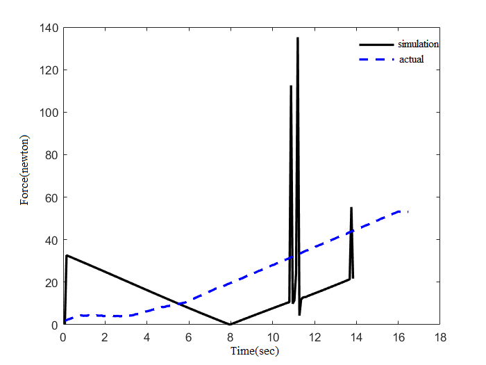
| − | + | The drive torque was simulated by ADAMS with the drive position at the center of the tyre unloader. Based on the actual radius of the tyre unloader being approximately 1 meter, it can be assumed that the dynamic ring thrust value is numerically equal to the drive torque value. The actual calculated dynamic ring thrust variation was compared with the simulated value of the tyre unloader motor drive ring and the comparison results are shown in [[#img-8|Figure 8]]. | |
| − | + | <div id='img-8'></div> | |
| − | + | {| class="wikitable" style="margin: 1em auto 0.1em auto;border-collapse: collapse;width:auto;" | |
| − | + | |-style="background:white;" | |
| − | + | |style="text-align: center;padding:10px;"| [[Image:Draft_Ling_717181314-image10.png]] | |
| + | |- | ||
| + | | style="background:#efefef;text-align:left;padding:10px;font-size: 85%;"| '''Figure 8'''. Comparison of simulated and actual values | ||
| + | |} | ||
| − | |||
| − | |||
| − | Due to the difference between the simulated and actual driving methods of the dynamic loops, the simulated and actual values are subject to certain errors. In ADAMS, a rotational drive is applied directly to the kinematic ring, and the simulation results from | + | Due to the difference between the simulated and actual driving methods of the dynamic loops, the simulated and actual values are subject to certain errors. In ADAMS, a rotational drive is applied directly to the kinematic ring, and the simulation results from [[#img-8|Figure 8]] show that the torque required to move the kinematic ring from rest to motion is large (0 to 0.1s), after which the drive torque required decreases (0.1 to 7.9s) due to the inertia of the kinematic ring itself. To maintain the movement, the torque will gradually increase, during which the collision between the moving ring and the guide wheel will also cause a sudden increase in torque, producing a peak (7.9 to 14s). In the actual working of the tyre unloader, the drive unit consists of three main parts: motor, reducer and screw. The specific mode of operation is by connecting the reducer to the motor in order to reduce the rotational speed and thus increase the output torque, which is converted into thrust on the screw by means of a screw to drive the moving ring for rotation. This process allows for customised settings of motor speed, output torque magnitude, etc. The torque magnitude is negligibly influenced by the interaction between the mechanisms during operation of the device. So the screw thrust tends to rise gradually and with little fluctuation. But the simulated force values are of the same order of magnitude as the actual force values, and the overall trend is gradually increasing, which proves that the simulation results have a certain degree of reasonableness. |
==3.4 Bearing transient dynamics analysis== | ==3.4 Bearing transient dynamics analysis== | ||
Revision as of 10:54, 14 April 2023
Abstract
Bearing is an important rotating support part of tyre unloader, and its fatigue reliability is an important part of the whole system reliability. Because of the huge alternating stress, the support bearing is required to have high fatigue life and reliability. In this paper, combined with stress-strength interference model and statistical theory, the life distribution of bearing steel material is predicted by using group test data; Based on the multi-rigid body dynamics and finite element numerical simulation platform, the reliability of the bearing of tyre unloader under different operating years was predicted by using the different dimensional interference model. The results show that the maximum resultant force of the bearing at the bottom rocker arm of the tyre unloader can reach 150kN, and the maximum transverse and longitudinal forces can reach 108kN and 78kN. When bearing the weight of the whole tyre and turning, the inertia force is the largest, the maximum stress value is 1316.2MPa, which occurs in the bearing inner ring and ball contact part. After the statistics, the stress amplitude distribution of the bearing conforms to Weibull distribution, and the life of the bearing follows lognormal distribution. After 105 tyre unloading, the fatigue reliability of the bearing is lower than 0.82, which is consistent with the actual working condition. Therefore, this model can be used to calculate the fatigue reliability of bearings conveniently and quickly, and provide certain theoretical support for the safety and fatigue reliability prediction of bearings.
Keywords: Numerical simulation, fatigue life, reliability, different dimensional interference model
1. Introduction
With the continuous improvement of China's machinery production process, the life and reliability of bearings has been greatly improved, but the bearings running on some large machinery, because of the huge alternating stress and complex working environment, making the life and reliability of bearings rapidly reduced. At the same time, with the rapid development of heavy machinery in China, the tonnage of tyres used is also rising. The object of this paper is a new type of giant tyre unloading machine, which unloads tyres weighing up to 6t. In the production process, the tyres need to be unloaded from a fixed position and flipped by the unloading machine after the completion of the previous process. During the unloading and flipping process, due to the huge weight of the tyre and the inertia force generated during the flipping, the tyre will collide and rub against the clamping mechanism of the tyre unloader, causing the system to vibrate and at the same time causing the bearings in key parts to be subjected to complex and variable random loads. Because of the randomness of the external load, the bearing material itself performance, size and other variability, the life distribution of bearings belongs to a probability distribution and with the growth of the use of years, bearing failure rate is on the rise. The reliability of the bearing life under different years needs to be studied to prevent bearing failure and subsequent safety accidents. The fatigue reliability of this new type of tyre unloader bearing is not systematically studied. In this paper, the fatigue reliability calculation method of the new tyre unloader bearing is proposed based on the theory of dynamic finite element and different dimensional interference model.
Current research on tyre unloaders is limited to the control methods and modes of operation. For example, Alessio et al. [1] introduced a robot that can assist tyre operators in the workshop to change tyres, which can be controlled in a variety of ways, such as automatic recognition of the user's gesture commands and remote operation through a control interface. In addition, Ján et al. [2] carried out a 3D modelling and dynamics analysis of a robot that unloads tyres, thus obtaining important mechanical parameters of the robot.
Existing bearing reliability predictions are different from the subject of this paper, and most of the analysis methods use isotropic interference models, which is the traditional stress-strength interference model. However, the strength distribution of general materials is difficult to predict and difficult to obtain strength distribution data through specific tests, and it needs to be combined with the material life distribution to obtain the strength distribution of materials through complex mathematical calculations, which is not conducive to the use of engineers. Domestic scholars Xie and Wang [3] proposed a heterogeneous interference model, which is no longer limited to the traditional reliability model in which the two variables must be of the same magnitude, but can be used to calculate the reliability through the stress distribution and the life distribution of the material. At the same time, the model no longer relies on tedious mathematical calculations but obtains the fatigue life distribution of the material through tests, which makes the fatigue reliability analysis much less difficult and simplifies the analysis steps. Liu et al. [4] provided a new analysis method for fatigue reliability of pipe structures by combining fatigue reliability of pipes under load with structural dynamic analysis. Zhou et al. [5] provided a theoretical basis for the life assessment and reliability analysis of rolling bearing systems through the fatigue reliability calculation formula of bearing systems under continuous load spectrum. Jin et al. [6] proposed an artificial intelligence method to analyze the fatigue reliability of aviation bearings. Qi and Liao [7] designed a system to evaluate the reliability of rolling bearings of traction motors based on MATLAB App Designer, which provided a new reference for the development and improvement of reliability evaluation systems.
Reuben et al. [8] improved this reliability assessment based on the Weibull diagram equation by estimating the variation in minimum bearing life and establishing confidence intervals using Monte Carlo simulations. Pape et al. [9] improved the calculation of bearing fatigue life by introducing residual stresses to the sub-surface region of the bearing. Wang [10] calculated the reliability life of ship unloader bearings by converting the tensile force of the ship unloader lifting mechanism into an average equivalent dynamic load on the bearings and then using the Miner criterion. Xia Xintao and Ye Liang et al. [11] proposed a new concept of rolling bearing performance retention reliability. Zhang et al. [12] established an analytical model for the contact fatigue reliability of main bearings based on the complex loading conditions of TBM main bearings and combined with fatigue cumulative damage and residual strength theory, based on a dynamic degradation model under complex conditions. Cheng et al. [13] developed a modified five-degree-of-freedom quasi-dynamic model considering multi-body interactions and used the modified fatigue life model proposed by Jones to assess the effect of angular displacement on bearing reliability. Herp et al. [14] proposed a bearing condition prediction method using temperature residuals and Bayesian probability statistics for wind turbine bearings, and this method can predict possible bearing failures within an average of 33 days. Tong et al. [15] proposed an improved model for calculating the operating torque of angular contact ball bearings (ACBB) by comparing the effect of different loading conditions on the fatigue reliability of angular misalignment on tapered roller bearings. König et al. [16] developed a model of bearing life which can determine the merits of hybrid bearings and allows for an analytical assessment of bearing life. Guillermo et al. [17] further extended a previously developed model for calculating bearing life based on high cycle fatigue by incorporating a new surface damage integral based on a creep mechanism into the model, providing a new approach to fatigue life prediction for bearings. Zhang et al. [18] used the maximum likelihood estimation method to calculate the actual value of the bearing, and used the SPSS curve and cumulative grey prediction model methods to train on some of the real data as a way of predicting the life of the bearing, and found that all three methods have some practical value in engineering, but the cumulative grey prediction was more effective. Lorenz et al. [19] developed a continuous damage mechanics (CDM) finite element (FE) model in order to investigate the effect of surface roughness on the rolling contact fatigue life of poor quality contact bodies and demonstrated the feasibility of the model. Pandey et al. [20] proposed a framework based on continuum damage mechanics and the finite element method to simulate the low circumferential fatigue crack expansion process, and developed a strain-based damage model to consider the effect of different strain ratios on fatigue damage. Cano et al. [21] developed a new intrinsic model for long-term prediction of creep deformation, damage and rupture by combining the Wilshire equation with continuum damage mechanics (CDM).
In summary, in terms of bearing reliability analysis and calculation, numerical analysis, theoretical calculation and experimental evaluation are mainly used at home and abroad to study the performance and life of various types of bearings, but there are fewer studies combining giant tyre unloaders and using heterogeneous interference models to analyse their bearing reliability. Therefore, this paper combines the existing information at home and abroad, mainly to fill the gap in the field of research on the fatigue reliability of bearings of giant tyre unloaders; Prediction of the life distribution of bearing steel materials using grouping method test data combined with statistical theory; Combining numerical simulation platforms such as dynamics and finite elements, the heterogeneous interference model is used to predict the reliability of bearings at different service lives. It also differs from traditional stress-strength interference models in that it directly uses the material life distribution for reliability calculations and is suitable for generalised applications in engineering.
2. Reliability analysis process
The fatigue reliability of the bearings of the giant tyre unloading machine is analysed and calculated by the numerical analysis platforms such as dynamics and finite element, using the theory related to fatigue reliability. The specific process is shown in Figure 1.

|
| Figure 1. Flow chart for calculating the fatigue reliability of a tyre unloader bearing |
3. Maximum stress history of bearing
3.1 Structure and modelling of the tyre unloader
The physical drawing of the tyre unloading machine is shown in Figure 2. Because of the complex structure of the tyre unloader proper, the model (with tyre 2) is shown in Figure 3 by simplifying the 3D modeling of the threads and other parts of the tyre unloader blank that will not have an impact on the final result.
| Figure 2. Physical view of the tyre unloader |

1. Clamping plate; 2. Tyres; 3. Guide wheels; 4. Fixed ring; 5. Dynamic ring; 6. Fixed ring rotary; 7. Rocker arm |
| Figure 3. 3D model of the tyre unloader |
The structure of the tyre unloader mainly consists of the Plywood 1, the Guide wheel 3, the Fixed ring 4, the Dynamic ring 5, the Rocker arm 7, etc. 16 pairs of rocker arms are mounted symmetrically on each side of the fixed ring, with the upper end connected to the moving ring by a linkage and the lower end connected to the cleat. The principle of operation is that the dynamic ring rotates at a certain angle with respect to the fixed ring, thus controlling the clamping plate on the rocker arm to clamp or unclamp the tyre. The fixed ring is equipped with 8 guide wheels, which support the fixed ring and guide it through a certain angle of rotation, while the rotation of the fixed ring and the turning of the machine are controlled by an electric motor.
3.2 Numerical simulation of the operating conditions of the tyre unloader
The above 3D model of the tyre unloader (including tyre) is imported into the dynamics analysis software ADAMS, and the material parameters of the model are set first. The material parameters of the whole machine and tyres are shown in Tables 1 and 2.
| Materials | Elastic modulus (MPa) | Poisson ratio | Density (kg/m3) |
|---|---|---|---|
| Rubber | 7.8 | 0.29 | 1200 |
| Materials | Elastic modulus (MPa) | Poisson ratio | Density (kg/m3) |
|---|---|---|---|
| Carbon structural steel | 207 | 0.29 | 7801 |
Constraint and actuation of each mechanism according to the actual motion of the tyre unloading machine. The whole mechanism of tyre unloading machine is mainly rotating sub and the connecting rod articulation, plywood and rocker arm and other rotating connections are rotating sub.The guidewheel shaft is fixed to the fixed ring using a fixed pair, and a rotating connection pair is applied between the guidewheel and the guidewheel shaft.The fixed ring and the moving ring are provided with a planar pair to prevent relative slippage caused by the rotation of the moving ring. To prevent over-constraints caused by the use of too many rotating subsets, resulting in instability of the solved system,the conflict constraints are replaced by primary subsets such as point overlap subsets or cylindrical amplitude, and coplanar subsets replace some of these planar subsets to ensure the stability and accuracy of the solved system.The virtual prototype of the tyre unloader is shown in Figure 4.

|
| Figure 4. Virtual prototype of the tyre unloader |
After building a virtual prototype of the tyre unloader system, the simulation is based on the actual working conditions of the tyre unloader. The simulation time is set as a cycle of 2.1s. After the simulation, the load spectrum of , and directions of the bearing at the bottom rocker arm is extracted, and the extraction position is illustrated in Figure 5. The loads in the and directions are transverse and longitudinal loads, and the loads in the direction are those perpendicular to the bearing outward. The extraction results are shown in Figure 6.

|
| Figure 5. Load extraction at rocker arm bearing |

|
| Figure 6. Three-way force load spectrum at rocker arm bearing |
According to the three-way force load spectrum, the average load in direction and direction of the bearing tends to 0 within 0.8s, and there is a certain impact load, which is caused by the vibration generated when the splint contacts the tyre. After the splint clamps the tyre, the fixing pair will temporarily fail. As the weight of the tyre itself is transferred to the bearing, the load values of the and directions of the bearing at the bottom rocker arm will rise rapidly. After about 0.2s, the components of the and directions increase and remain at about 108kN and 78kN, respectively.
3.3 Validation of simulation results
Because the simulation analysis model is simplified to some extent, the simulation results have some errors.Therefore, in order to verify the reasonableness and realism of the simulation results and to provide a reasonable dynamic load spectrum for the subsequent analysis and prediction of the bearing reliability. Through the proportional coefficient of the real-time output torque of the clamping motor on the control panel of the tyre unloader (Figure 7), the output torque coefficient of the motor is converted into the actual moving ring thrust of the tyre unloader and compared with the simulation value of ADAMS, and the reasons for the error between the actual value and the simulation result are analyzed.

|
| Figure 7. Tyre unloader control panel |
The comparison data in the test is the thrust of the tyre unloading maneuver ring, which is the current torque value of the birth ring in the picture. The output proportional coefficient needs to be converted into the real thrust force on the moving ring, namely the lead screw thrust. The relation between output torque of reducer and motor parameters is shown in Eq. (1)
|
|
(1) |
where represents the motor power, which is 0.75kW, represents the motor speed, which is 1500r/min, represents the transmission efficiency, which is 98%, and represents the speed ratio of motor and reducer, which is 20:1.
The maximum output torque of reducer is 94N m.
The conversion formula between output torque of reducer and thrust Fa of the lead screw is shown in Eq. (2). The maximum thrust force Fa of the screw is calculated from the maximum output torque to be 56 N. The motor torque output scaling factor is converted into a value for the change in thrust of the kinematic ring, the torque factor and the actual kinematic ring thrust values are shown in Table 3
|
|
(2) |
where is the lead of the lead screw, which is 10mm, and represents the conversion efficiency, which is 95%.
| Proportional coefficient of output torque (‰) | Actual moving ring thrust (N)</span> |
|---|---|
| 232 | 12.99 |
| 239 | 13.38 |
| 244 | 13.66 |
| 250 | 14.00 |
| 258 | 14.45 |
| 262< | 14.67 |
| 269 | 15.06 |
| 276 | 15.46 |
| 283 | 15.85 |
| 289 | 16.18 |
| 295 | 16.52 |
| 304 | 17.02 |
| 302 | 16.91 |
| 309 | 17.30 |
| 317 | 17.75 |
| 321 | 17.98 |
| 327 | 18.31 |
The drive torque was simulated by ADAMS with the drive position at the center of the tyre unloader. Based on the actual radius of the tyre unloader being approximately 1 meter, it can be assumed that the dynamic ring thrust value is numerically equal to the drive torque value. The actual calculated dynamic ring thrust variation was compared with the simulated value of the tyre unloader motor drive ring and the comparison results are shown in Figure 8.
|
| Figure 8. Comparison of simulated and actual values |
Due to the difference between the simulated and actual driving methods of the dynamic loops, the simulated and actual values are subject to certain errors. In ADAMS, a rotational drive is applied directly to the kinematic ring, and the simulation results from Figure 8 show that the torque required to move the kinematic ring from rest to motion is large (0 to 0.1s), after which the drive torque required decreases (0.1 to 7.9s) due to the inertia of the kinematic ring itself. To maintain the movement, the torque will gradually increase, during which the collision between the moving ring and the guide wheel will also cause a sudden increase in torque, producing a peak (7.9 to 14s). In the actual working of the tyre unloader, the drive unit consists of three main parts: motor, reducer and screw. The specific mode of operation is by connecting the reducer to the motor in order to reduce the rotational speed and thus increase the output torque, which is converted into thrust on the screw by means of a screw to drive the moving ring for rotation. This process allows for customised settings of motor speed, output torque magnitude, etc. The torque magnitude is negligibly influenced by the interaction between the mechanisms during operation of the device. So the screw thrust tends to rise gradually and with little fluctuation. But the simulated force values are of the same order of magnitude as the actual force values, and the overall trend is gradually increasing, which proves that the simulation results have a certain degree of reasonableness.
3.4 Bearing transient dynamics analysis
From the results of the kinetic analysis, it can be seen that the bearing at the lowermost rocker is subjected to the greatest component of gravity of the tyre blank and is also furthest from the centre of rotation, where the centrifugal inertia force is greatest. The bearing selected here for analysis is therefore a deep groove ball bearing, type 61918. The bearing model is shown in Fig. 9. According to the actual bearing size parameters, the 3D modelling software is used to establish a 3D model of the bearing at the rocker arm. In order to simplify the calculation steps and save calculation resources, non-important parts such as the cage are omitted, the bearing dimensional parameters are shown in Table 4.
| Bearing type | Outer diameter(mm) | Inner diameter(mm) | Thickness(mm) |
| 61918 | 125 | 90 | 18 |
The bearing model was imported into Ansys finite element analysis software, the inner and outer rings of the bearing were constrained, and the bearing material parameters were set, as shown in Table 5. The extracted X, Y and Z forces are loaded onto the corresponding parts of the bearing for transient dynamics analysis, with the loads and constraints applied as shown in Fig. 10. The results of the transient dynamics analysis (equivalent stress clouds) are shown in Fig. 11.
| Materials | Elastic Modulus
(MPa) |
Poisson
ratio |
Yield Strength(MPa) | Tensile strength(MPa) | ||
| GCr15 | 210000 | 0.29 | 1458 | 1617 | ||
The bearing of the lowermost rocker arm of the tyre unloader is subjected to the greatest inertial force when carrying the weight of the entyre tyre and turning it over. From the results of the transient dynamics analysis, it can be seen that the maximum stress value that the bearing is subjected to is 1316.2Mpa, so the part of the bearing where the stress is high and easy to produce fatigue is the inner ring and ball contact.
3.5 Stress history in hazardous areas
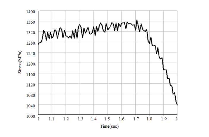
In order to obtain the distribution characteristics of the stresses in the hazardous parts of the bearings, the ANSYS APDL was used to extract the nodal stress time histories corresponding to the fatigue parts of the bearings according to the results of the transient dynamics. The curve for the change in stress history is shown in Fig. 12.4. Bearing reliability calculation based on heterogeneous interference model
4.1 Stress history rain flow count statistics
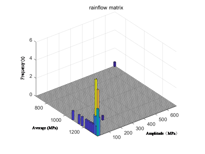
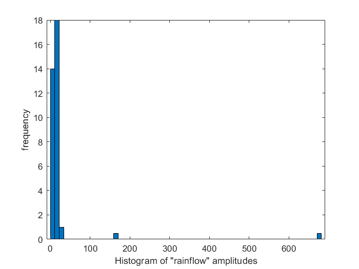
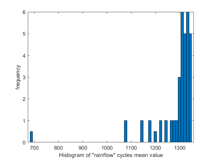
From the basic theory of fatigue, it can be seen that the load average, amplitude and the number of cycles are the main factors that make the component produce fatigue damage, so the bearing fatigue part of the stress time course need to be cycle counting process. In this paper, the two-parameter rainfall counting method is used to count the amplitude and mean values of the loads and to obtain important relationships between the load amplitude, mean value and the corresponding frequency.
Rain flow counting of the stress history was carried out to convert the random variable amplitude stress into a series of load cycles, the amplitude and mean distribution of the load cycles were counted and the mean and amplitude were converted into a two-dimensional histogram and the statistical results are shown in Fig. 13- Fig. 15.
Using Goodman's theory to apply an average stress correction to the stress amplitude, the stress state is converted to a load cycle with a stress ratio of -1, according to an equal life, the corrected load cycles were used as equivalent stresses for the next step of the fatigue reliability analysis. The Goodman formula is shown in Eq. (3) and the corrected results are shown in Fig. 16.
|
|
(3) |
Where σa denotes the actual working stress amplitude (MPa).
σm indicates the average stress in actual working conditions (Mpa).
σb indicates the tensile ultimate strength of the material (MPa).
σ-1 denotes the stress magnitude (MPa) for a stress ratio of -1.
4.2 Load amplitude probability distribution fitting and test
Due to the influence of factors such as short sampling time and large amount of data in compiling load spectrum, the load history obtained cannot fully reflect the actual load history of the bearing in the whole life stage, therefore, in order to improve the reliability of the results, the probability distribution function of random loads should be calculated, and then the load distribution of bearings in the whole life interval should be predicted.
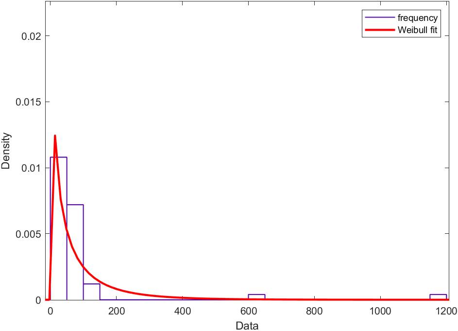
According to the rain-flow counting statistics of stress time history in fatigue parts of bearings, the probability statistics of stress amplitude are carried out and fitted by Weibull distribution. The fitting effect and test results are shown in Fig. 17. It can be seen that the distribution of stress amplitudes generally conforms to the Weibull distribution.
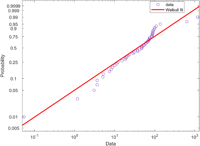
In order to verify whether the stress amplitude conforms to Weibull distribution, Fig. 18 is obtained by the graphical method. It can be concluded from the figure that the closer the data is to a straight line, the better the data fitting effect is. Therefore, it can be considered that the probability density function of stress amplitude conforms to Weibull distribution.
Using the great likelihood method to solve for the Weibull correlation parameters, the relevant solution parameters are shown in Table 6.
| Scale parameterse parameters | Shape parameters | Confidence level |
| 61.93 | 0.729 | 0.05 |
The equivalent load probability density function is:
|
(4) |
Where β denotes the shape parameter, θ denotes the scale parameter. Substituting the two into Eq. (4) gives:
|
|
(5) |
4.3 Material life distribution of bearing steel under arbitrary stress
A set of fatigue test data for bearing steel was obtained from the literature[22] and combined with Basquin's equation to derive a continuous probability life model for bearing steel using the great likelihood method. The test material was a high-carbon chromium bearing steel with the chemical composition shown in Table 7, which was machined to give the dimensions in Fig. 19. Then using the grouping method, a four-linked cantilever beam type rotating bending fatigue tester was used to carry out the test, starting with a load of 1700 MPa stress. By reducing the weights so that the stresses fell at intervals of 50 to 100 MPa, nine sets of fatigue test data were eventually obtained, as shown in Table 8.
| Element | C | Si | Mn | Cr | Cu | Ni | Mo | P | S |
| Content % | 1.01 | 0.23 | 0.36 | 1.45 | 0.06 | 0.04 | 0.02 | 0.01 | 0.007 |
| Stress(MPa) | Life
(cycle) |
Stress
(MPa) |
Life
(cycle) |
| 1700 | 4480 | 1300 | 2480000 |
| 6100 | 3870000 | ||
| 6840 | 1250 | 40560 | |
| 1600 | 5200 | 52430 | |
| 7790 | 65990 | ||
| 10000 | 128800 | ||
| 1500 | 8990 | 2486740 | |
| 14400 | 4983540 | ||
| 34700 | 8950470 | ||
| 247000 | 10325090 | ||
| 609000 | 11730550 | ||
| 1400 | 13460 | 26058040 | |
| 15900 | 1200 | 125280 | |
| 17220 | 269929 | ||
| 40800 | 672410 | ||
| 839140 | 8771540 | ||
| 1540000 | 19548550 | ||
| 4970760 | 41502050 | ||
| 1300 | 15360 | 43386180 | |
| 22670 | 61683430 | ||
| 39830 | 1150 | 23276820 | |
| 2050180 | 47700000 |
Due to some differences in the actual size, shape and working conditions of the tyre unloader bearings used in this study and the shape and loading method used for the test specimens, therefore, the S-N relationship for the test material needs to be corrected to the S-N relationship for the actual zero component, and the correction formula is as follows:
|
|
(6) |
Where, corresponds to the stress tested in the material;
corresponds to zero component stress;
is the dimensional coefficient of the material, the value of 0.856 was taken by consulting the 《Mechanical Design Manual》.
β is the material surface quality factor, here taken as 1.
is the loading method for the workpiece and the steel tension is taken as 0.85.
The fatigue notch coefficient K_f is related to the stress concentration coefficient, the bearing stress concentration is generally related to the roughness, here it can be considered that the bearing is consistent with the roughness of the test piece, take the value of 1, the correction results are shown in Table 9.
| Test stress(MPa) | Corrected stress(MPa) |
| 1700 | 1030 |
| 1600 | 970 |
| 1500 | 909 |
| 1400 | 849 |
| 1300 | 788 |
| 1250 | 758 |
| 1200 | 728 |
| 1150 | 697 |
4.4 Maximum likelihood method for determining the P-S-N curve of bearing steel
The general material fatigue life follows a log-normal distribution. Assuming that the bearing steel life follows a log-normal distribution, the Anderson-Darling hypothesis test was performed on the fatigue test data at different stresses in Table 8. As the A-D test can take different confidence intervals for testing, the smaller the confidence interval, the more obvious the test effect. So 95% confidence intervals were taken for hypothesis testing of each group of fatigue data, and the test results are shown in Fig. 20- Fig. 21(partial) and Table 10(all).
| Proof stress(MPa) | AD | P value |
| 1030 | 0.264 | 0.371 |
| 970 | 0.210 | 0.544 |
| 909 | 0.279 | 0.484 |
| 849 | 0.562 | 0.091 |
| 788 | 0.603 | 0.062 |
| 758 | 0.735 | 0.037 |
| 728 | 0.707 | 0.042 |
| 697 | 0.250 | 0.277 |
The test shows that the p-value is greater than the significant level of 0.05, which is in line with the hypothesis test, and therefore the bearing steel material life can be considered to be in line with the log-normal distribution.
The S-N curve of the bearing is estimated using Basquin's equation combined with the method of great likelihood, Basquin's equation is
|
|
(7) |
Where m is the exponent, N is the fatigue life and C is a constant.
Taking the logarithm of both sides gives:
|
|
(8) |
Where the subscript p indicates the survival rate.
When the survival rate is 50%, the median log life is equal to the mean of the log life:
|
|
(9) |
Where is the mean log life of the sample at different stress.
When S=788MPa, the mean value of the log-life sample with stress of 788MPa is substituted as the parent mean value in Eq. (8) and (9) to obtain.
|
|
(10) |
|
|
(11) |
The log life of bearing steel follows a normal distribution and the mean log life is related to the standard deviation of the log life at different survival rates as follows:
|
|
(12) |
Where is the standard deviation of the log life of the member at different stress. is the standard normal deviation corresponding to the probability of damage.
Substituting Eq, (8) and (9) into Eq. 12 yields:
|
|
(13) |
The sample log life standard deviation at a stress of 788Mpa is substituted into Eq. (13) as the parent log life standard deviation:
|
|
(14) |
Also known as equation:
|
|
(15) |
When the survival rate P = 84.1%,υ_p=1, which is collated to give:
|
|
(16) |
When N follows a log-normal distribution, its probability density function is
|
|
(17) |
Substituting the different stresses and corresponding lifetimes into Eq. (17) and multiplying them together, the likelihood function is obtained as equation
|
|
(18) |
Take the logarithm on both sides of the above equation, and get it
|
|
(19) |
Convert Eq. (18) into Eq. (19) and find the minimum value of equation (19) to find the maximum value of the likelihood function equation
|
|
(20) |
Find the minimum value of F to obtain the maximum likelihood estimates of the parameters m50,m84.1, m50=15.04, m84.1=5.32.
The values of parameters m50 and m84.1 are substituted into Eq. (11) and Eq. (16) respectively to obtain the life distribution parameters under any stress, and the log life mean and standard deviation parameter equations are as follows:
|
|
(21) |
|
|
(22) |
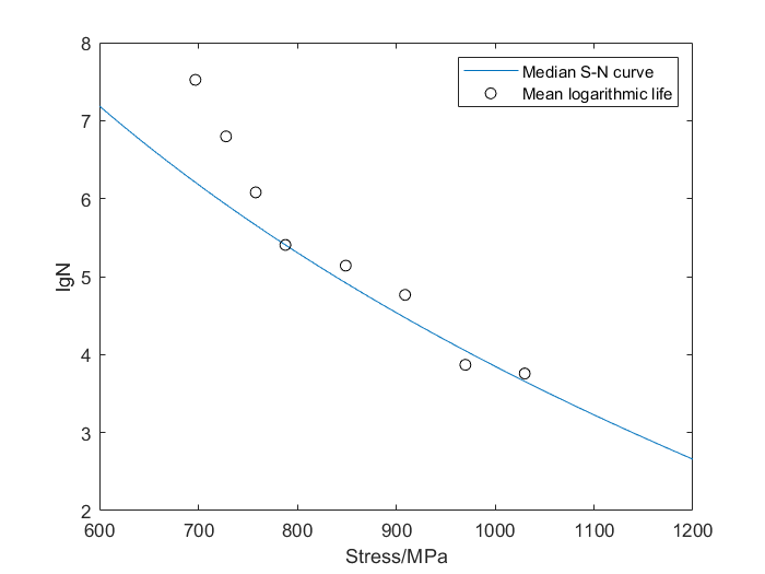
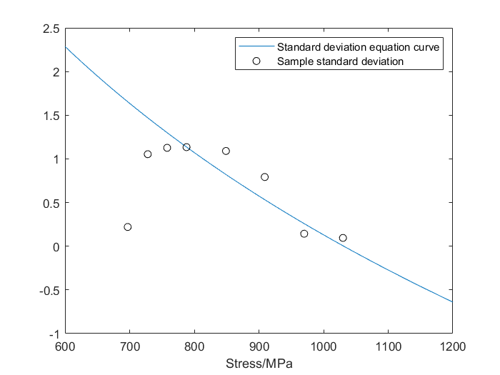
The parameter-stress equation derived by the great likelihood method was plotted against the sample log-life mean and standard deviation in the same graph for comparison. The sample log-life mean and log-life standard deviation are shown in Table 11 and the results of the comparison are shown in Fig. 22 - Fig. 23. Within a certain interval, the fit is good, which proves that the parameter equations derived using the great likelihood method are more reasonable.
| Stress (MPa ) | Mean log -life | Standard deviation of log-life |
| 1030 | 3.7572 | 0.0951 |
| 970 | 3.8692 | 0.1433 |
| 990 | 4.766 | 0.7922 |
| 849 | 5.1407 | 1.0905 |
| 788 | 5.406 | 1.1344 |
| 758 | 6.0801 | 1.1266 |
| 728 | 6.7981 | 1.0539 |
| 697 | 7.5227 | 0.2203 |
5. Bearing fatigue reliability
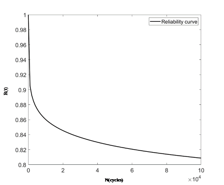
According to the heterogeneous interference model, for different reliability of fatigue life is calculated, the model as shown in the equation, the above calculated stress distribution Eq. (4) and life distribution Eq. (17) substituted into the following Eq. (23), the fatigue life curve of the bearing can be obtained as shown in Fig. 24.
|
|
(23) |
Where R is the fatigue reliability, h(S) is the probability density function of the equivalent load distribution and f(n,S) is the probability density function of the component life under different stresses.
As can be seen from Figure 24, the fatigue reliability decreases continuously with increasing fatigue life, which is consistent with reality. The downward trend is faster until the number of cycles is 105, after which it slows down. When the number of fatigue cycles reaches 105, the fatigue reliability of the bearing drops to below 0.82.
6. Conclusions
In this paper, the reliability of the bearings of a giant tyre unloader is predicted using a multi-body dynamics, finite and other numerical simulation platform, combined with a heterogeneous interference model, for a huge alternating load during operation:
(1) The joint simulation between ADAMS and ANSYS shows that the combined force on the bearing at the lowermost rocker arm of the tyre unloader can reach a maximum of 150kN, with a maximum of 108kN and 78kN in the transverse and longitudinal directions. The bearing of the lowermost rocker arm of the tyre unloader is subjected to the greatest inertial force when bearing the weight of the whole tyre and flipping, and the maximum stress value is 1316.2Mpa.
(2) By probability fitting and testing, the equivalent stress distribution in the fatigue part of the bearing conforms to the Weibull distribution, with the Weibull distribution scale parameter and shape parameter being 61.93 and 0.72 respectively at a confidence interval of 95%.
(3) Under the modified S-N curve, the life of the bearing steel material under any stress conforms to a log-
normal distribution, and the Basquin equation exponents are 15.04 and 5.32 for a survival rate of 50% and 84.1% respectively, as obtained by the maximum likelihood method.
(4) Based on the heterogeneous interference fatigue reliability model and according to the reliability calculation results, the reliability of the bearing shows a decreasing trend with the increase of the number of times it is used, which is in line with the actual situation, when the service life of the bearing reaches 105 times, the reliability drops to below 0.82.
The kinetic simulation, finite element analysis, fatigue reliability prediction and other technical methods used in this paper are feasible for the fatigue reliability prediction of tyre unloading machine bearings.
Funding This work was supported by the Natural Science Foundation of Fujian Province (Grant No.2020J01871), China Postdoctoral Science Foundation (Granted No.2020M671956).
Declarations
Conflict of Interests Conflict of interests The authors declare that they have no known competing financial interests or personal relationships.
References
[1] Levratti A , Riggio G , Fantuzzi C, et al. tyreBOT: A collaborative robot for the tyre workshop [J]. Robotics and Computer-Integrated Manufacturing,2019, 57(JUN.) :129-137. https://doi.org/10.1016/j.rcim.2018.11.001
[2] Vavro J , Vavro J , Kováiková, Petra, et al. Kinematic and Dynamic Analysis of the Manipulator for Removal of Rough Tyres [J]. Procedia Engineering, 2016, 136 :120-124. https://doi.org/10.1016/j.proeng.2016.01.184
[3] Xie L.Y, Wang Z. Heterogeneous interference model for fatigue reliability with random constant amplitude cyclic loading [J]. Journal of Mechanical Engineering,2008(01) :1-6(in Chinese).
[4] Liu K, Wang M, Yang G L. Fatigue reliability analysis of underground pipeline structures under multiple operating conditions [J]. Safety and Environmental Engineering,2019,26(04) :106-110+126(in Chinese). https://doi.org/10.13578/j.cnki.issn.1671-1556.2019.04.017
[5] Li R X, Zhou J Y, Sun K Z,et al. Fatigue reliability analysis of rolling bearing systems under random loading [J]. Hydromechatronics Engineering,2012,40(01) :157-160(in Chinese).
[6] Jin Y, Liu S J, Zhang J G. Fatigue reliability of high-speed rolling bearings under artificial neural network based on ge-etic algorithm optimization [J]. Journal of Aerospace Power,2018,(11) :2748-2755(in Chinese). https://doi.org/10.13224/j.cnki.jasp.2018.11.021
[7] Qi M Y, Liao A H. Design of a MATLAB App Designer based rolling bearing reliability assessment system for traction motors [J]. Electronics Technology,2022,(03) :79-86(in Chinese). https://doi.org/10.16180/j.cnki.issn1007-7820.2022.03.012
[8] Lim Chi Keong Reuben, Michael Corsar, David Mba. Bearing replacement extension without failure data[J]. Int. J. of Risk Assessment and Management, 2015, 18(1) : 38-51. https://doi.org/10.1504/IJRAM.2015.068139
[9] F. Pape, O. Maiss, B. Denkena, G. Poll, et al. Computational approach to improve bearings by residual stresses based on their required bearing fatigue life[J]. International Journal of Computational Methods and Experimental Measurements, 2017(4), : 656-666. https://doi.org/10.2495/CMEM-V6-N4-656-666
[10] Wang H B. Ship unloader rolling bearing life prediction and maintenance management platform development [D]. Jilin University,2011(in Chinese).
[11] Xia X T, Ye L et al. Prediction of rolling bearing performance retention reliability [J]. Bearings,2016,(06) :28-34(in Chinese). https://doi.org/10.19533/j.issn1000-3762.2016.06.008
[12] Zhang X, Zhang Y Q, Sun Y, et al. Reliability Model of TBM Main Bearing based on Nonlinear Strength Degradation Theory[J]. International Journal of Performability Engineering,2018,14(12) :3054-3065. https://doi.org/10.23940/ijpe.18.12.p15.30543065
[13] Cheng W W, Xiang M H, Lyu Bugao et al. Influence of angular misalignment on the tribological performance of high-speed micro ball bearings considering full multibody interactions[J]. Proceedings of the Institution of Mechanical Engineers, Part J: Journal of Engineering Tribology,2021,235(6) :1168-1189. https://doi.org/10.1177/1350650120948292
[14] Herp J, Ramezani M H , Bach-Andersen M, et al. Bayesian state prediction of wind turbine bearing failure[J]. Renewable Energy,2018,116 :164-172. https://doi.org/10.1016/j.renene.2017.02.069
[15] Tong V C,Hong S W. Improved formulation for running torque in angular contact ball bearings[J]. International Journal of Precision Engineering and Manufacturing,2018,19(1) :47-56. https://doi.org/10.1007/s12541-018-0006-2
[16] König F, Ouald C A, Jacobs G, et al. A multiscale-approach for wear prediction in journal bearing systems – from wearing-in towards steady-state wear[J]. Wear,2019,426-427. https://doi.org/10.1016/j.wear.2019.01.036
[17] Guillermo E, Gabelli A. A model for rolling bearing life with surface and subsurface survival: Surface thermal effects[J]. Wear,2020 : 203446. https://doi.org/10.1016/j.wear.2020.203446
[18] Zhang Y C, Shu T, Ding R X. Bearing Life Prediction Based on SPSS and Grey Prediction Model[J]. IOP Conference Series: Earth and Environmental Science,2021,634(1) :012051. https://doi.org/10.1088/1755-1315/634/1/012051
[19] Lorenz S J, Sadeghi F, Trivedi H K, et al. A Continuum Damage Mechanics Finite Element Model for Investigating Effects of Surface Roughness on Rolling Contact Fatigue[J]. International Journal of Fatigue,2020,143(3) :105986. https://doi.org/10.1016/j.ijfatigue.2020.105986
[20] Pandey V B , Singh I V , Mishra B K . A Strain-based Continuum Damage Model for Low Cycle Fatigue under Different Strain Ratios[J]. Engineering Fracture Mechanics, 2020, 242(4):107479. https://doi.org/10.1016/j.engfracmech.2020.107479
[21] Cano J A , Stewart C M . A continuum damage mechanics (CDM) based Wilshire model for creep deformation, damage, and rupture prediction[J]. Materials Science and Engineering A, 2021, 799(4):140231. https://doi.org/10.1016/j.msea.2020.140231
[22] Li W, Lu L T. Probabilistic properties of the ultra-long life S-N relationship for high-carbon chromium bearing steels [J]. Journal of Traffic and Transportation Engineering,2006(02):17-21(in Chinese).Document information
Published on 18/04/23
Accepted on 10/04/23
Submitted on 24/02/23
Volume 39, Issue 2, 2023
DOI: 10.23967/j.rimni.2023.04.001
Licence: CC BY-NC-SA license
Share this document
claim authorship
Are you one of the authors of this document?


