| Line 194: | Line 194: | ||
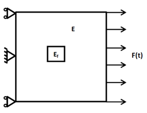
When projecting into this reduced basis the measured field, undamaged regions are expected being better approximated that the ones in which damage occurs. Thus, data-mining strategies could be then used to differentiate both regions (undamaged and damaged depicted in Figure [[#img-1|1]]). | When projecting into this reduced basis the measured field, undamaged regions are expected being better approximated that the ones in which damage occurs. Thus, data-mining strategies could be then used to differentiate both regions (undamaged and damaged depicted in Figure [[#img-1|1]]). | ||
| − | For that purpose, problem ([[#eq-7|7]]) is solved with the same geometrical and mechanical properties defined in | + | For that purpose, problem ([[#eq-7|7]]) is solved with the same geometrical and mechanical properties defined in [[#table-1|Table 1]] but without any damaged zone. |
By solving the discret equation ([[#eq-9|9]]) we obtain the undamaged displacement field <math display="inline">\mathbf u(\mathbf{x},t)</math> and from it the displacement field norm <math display="inline">w(\mathbf{x},t)</math> at the nodes <math display="inline">\mathbf{x}_i</math> of the spatial mesh at times <math display="inline">t_m = m \cdot \Delta t</math>, with <math display="inline">i \in [1,\dots ,N]</math> and <math display="inline">m \in [0,\dots ,M]</math>. In the sequel we use the notation <math display="inline">w(\mathbf{x}_i,t_m) \equiv w_i^m</math>, and <math display="inline">\mathbf{w}^m</math> represents the vector of nodal values <math display="inline">w_i^m</math> at time <math display="inline">t_m</math>. | By solving the discret equation ([[#eq-9|9]]) we obtain the undamaged displacement field <math display="inline">\mathbf u(\mathbf{x},t)</math> and from it the displacement field norm <math display="inline">w(\mathbf{x},t)</math> at the nodes <math display="inline">\mathbf{x}_i</math> of the spatial mesh at times <math display="inline">t_m = m \cdot \Delta t</math>, with <math display="inline">i \in [1,\dots ,N]</math> and <math display="inline">m \in [0,\dots ,M]</math>. In the sequel we use the notation <math display="inline">w(\mathbf{x}_i,t_m) \equiv w_i^m</math>, and <math display="inline">\mathbf{w}^m</math> represents the vector of nodal values <math display="inline">w_i^m</math> at time <math display="inline">t_m</math>. | ||
| Line 337: | Line 337: | ||
In order to reduce the dimensionality before applying the clustering, PCA is applied on the absolute value of the residual vectors. | In order to reduce the dimensionality before applying the clustering, PCA is applied on the absolute value of the residual vectors. | ||
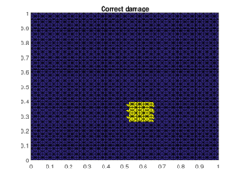
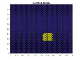
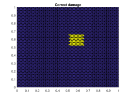
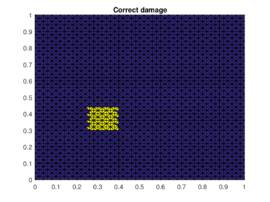
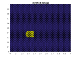
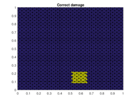
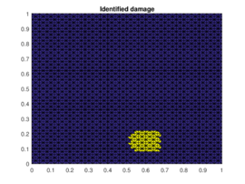
| − | The results of the damaged zone predicted by the proposed method for different positions of the damage are presented in | + | The results of the damaged zone predicted by the proposed method for different positions of the damage are presented in [[#img-2|Figures 2]] and [[#img-3|3]]. We can see how it detects quite precisely the position of damaged regions. Moreover in [[#img-4|Figure 4]] one can see how even if the reduction of dimension performed by the PCA is extreme (only the three first principal components are taken) the zones (damaged and undamaged) are perfectly differentiated. |
<div id='img-2a'></div> | <div id='img-2a'></div> | ||
| Line 357: | Line 357: | ||
| (c) | | (c) | ||
|- style="text-align: center; font-size: 75%;" | |- style="text-align: center; font-size: 75%;" | ||
| − | | colspan="2" | '''Figure 2 | + | | colspan="2" | '''Figure 2'''. Prediction versus reference damage location for the first three different positions of the damaged zone |
|} | |} | ||
| Line 377: | Line 377: | ||
| (d) | | (d) | ||
|- style="text-align: center; font-size: 75%;" | |- style="text-align: center; font-size: 75%;" | ||
| − | | colspan="2" | '''Figure 3 | + | | colspan="2" | '''Figure 3'''. Prediction versus reference damage location for the last two different positions of the damaged zone |
|} | |} | ||
| Line 386: | Line 386: | ||
|[[Image:review_Quaranta_et_al_2018a-identified_pca_complete_5.png|270px|First three principal components of the absolute value of the residual field for case (b) of Figure [[#img-2|2]]. Red points belong to the damaged zone.]] | |[[Image:review_Quaranta_et_al_2018a-identified_pca_complete_5.png|270px|First three principal components of the absolute value of the residual field for case (b) of Figure [[#img-2|2]]. Red points belong to the damaged zone.]] | ||
|- style="text-align: center; font-size: 75%;" | |- style="text-align: center; font-size: 75%;" | ||
| − | | colspan="2" | '''Figure 4 | + | | colspan="2" | '''Figure 4'''. First three principal components of the absolute value of the residual field for case (b) of Figure [[#img-2|2]]. Red points belong to the damaged zone |
|} | |} | ||
Revision as of 13:25, 7 July 2021
Abstract
Structural Health Monitoring is of major interest in many areas of structural mechanics. This paper presents a new approach based on the combination of dimensionality reduction and data-mining techniques able to differentiate damaged and undamaged regions in a given structure. Indeed, existence, severity (size) and location of damage can be efficiently estimated from collected data at some locations from which the fields of interest are completed before the analysis based on machine learning and dimensionality reduction techniques proceed.
Keywords: Non destructive testing, machine learning, dimensionality reduction
1. Introduction
Structural deterioration and degradation are of great concern worldwide, being damage the main cause of structural failure. A special attention must be paid in order to avoid the sudden failure of structural components. The improvements in the fields of low-cost displacement and acceleration transducers, signal conditioning and sampling hardware, electronic data acquisition systems, pushed the interest of the scientific community in the use of the dynamic response of structural systems as a tool to evaluate damage and safety. Recently, various non-destructive techniques based on changes in the structural vibrations patterns have been extensively published not only to detect the presence of damage but also to identify the location and the severity of it. Non-destructive Testing (NDT) methods are one of the most important topics in the Structural Health Monitoring (SHM) field. These methods have to be able to identify damage when it appears and capture and locate the damaged area.
Several system identification techniques exist to obtain unknown structural parameters as damping ratio, natural frequencies or mode shapes [1,2]. The basis of these methods is to extract information from some measurements on the structure, as, for example, accelerations or displacements. A first classification divides the methods in frequency domain and time domain methods.
Frequency domain techniques have the advantage of modal analysis methods, where the analysis can be done in some range of frequencies of interest or with some structural modes. In [3,4,5,6,7] frequency domain responses are obtained from time series responses by non-parametric estimation and signal processing techniques which make use of the Fourier transform. Concerning modal analysis methods [8,9,10,11,12,13,14] they are based on the use of modal informations extracted from input-output measurements by means of the modal analysis methods or from only output data measured under the ambient excitation (wind, traffic loads, etc.) without making use of artificial forces.
Time domain methods avoid problems as leakage or closeness to natural frequencies. In [2, 15,16,17,18,19,20] authors identified modal parameters from time domain measurements and used the extracted vibration features and modal properties for detecting damage occurrence and/or location by comparing the identified modal properties with the original values. It is also possible with these methods [21,22,23] to directly detect damage based on the measured data. Another approach in this group [24,25,26] makes use of many signal processing techniques and artificial intelligence as analysis tools to investigate the vibration signals and extract features to represent the signal characteristics.
Another classification could be done depending on the nature of the excitation force: some methods work with a known impulse force [27], others work with unknown natural excitations [28], and a third group works with a combination of the previous ones [29].
Wavelet analysis is also an appealing technique widely used for the Non-Destructive Testing, in which a wavelet transform is applied on modal shapes of vibration. Since this analysis is capable to identify changes in the modal shapes, damage can be easily identified as well as its spatial location. There is a vast literature on the extensive use of wavelets [30,31,32,33,34,35,36,37].
Reduced Order Modeling (ROM) techniques have been widely used in order to locate damage under real-time constraints. In the field of SHM there exists lots of approaches making use of reduced order modeling. In [38] authors applied the Proper Orthogonal Decomposition (POD) to track the structural behavior followed by an improved particle filtering strategy (extended Kalman updating). Machine learning is also helping for extracting the manifold in which the solutions of complex and coupled engineering problems are living. Thus, uncorrelated parameters can be efficiently extracted from the collected data coming from numerical simulations, experiments or even from the data collected from adequate measurement devices. The Proper Orthogonal Decomposition (POD), that is equivalent to Principal Components Analysis (PCA), can be viewed as an information extractor from a data set that attempts to find a linear subspace of lower dimensionality than the original space. Moreover, PCA-based transformations preserve distances, where other nonlinear dimensionality reduction strategies fail to accomplish it. In [39] authors proposed a data-driven methodology for the detection and classification of damages by using multivariate data driven approaches and PCA. Support Vector Machine (SVM) was used for damage detection in [40].
It is also usual in this context approaches that combine Machine Learning Techniques and Reduced Order Modeling, like in [41] where authors used machine-learning algorithms to generate a classifier that monitors the damage state of the system and a Reduced Basis method to reduce the computational burden associated with model evaluations. Proper Orthogonal Decomposition approximations and Self-Organizing Maps (SOM) are combined to realize a fast mapping from measured quantities in order to propose a data-driven strategy to assist online rapid decision-making for an unmanned aerial vehicle that uses sensed data to estimate its structural state [42].
Data Mining techniques are also used in the context of the SHM. In [43] authors propose an approach for damage identification and optimal sensor placement in Structural Health Monitoring by using a Genetic Algorithm technique (GA) whereas in [44] authors combined Data Mining (GA), Machine Learning (PCA) and Deep Learning (Neural Networks) techniques in the damage identification context. Concerning Deep Learning techniques, it is interesting the work developed in [45] in which a smart monitoring of aeronautical composites plates based on electromechanical impedance measurements and artificial neural networks is presented. At its turn [46] proposes the same technique in the monitoring of a frame structure model for damage identification.
This paper proposes a new strategy based on the combination of model order reduction, that extracts a reduced basis from undamaged snapshots, that will serve for projecting any measured solution on it, with data-mining techniques. When projecting into this reduced basis the measured field, undamaged regions are expected being better approximated that the ones in which damage occurs. Thus, data-mining strategies could be then used to differentiate both regions (undamaged and damaged). Finally, in order to limit the number of points at which data is collected, the just described methodology is combined with a data-completion strategy based on the use of dictionary learning.
After this short introduction, next section addresses the data generator based on the solution of a elastodynamic model in a plate. Then, next section applies different techniques on the generated data in order to clusterize damaged and undamaged zones. Finally the same procedure is repeated but on the completed data obtained from data sparsely collected.
2. Elastodynamic model
The problem taken into consideration is depicted in Figure 1. The geometrical and mechanical properties of the square domain are defined in Table 1.
|
| Figure 1. The 2D model |
| : Length () | |
| : Young modulus () | |
| : Poisson coefficient |
A linear elastic behavior is assumed in the undamaged area, so that the relation between the stress and the strain reads
|
|
(1) |
where is the Hooke's fourth order tensor. The relation between strain and displacement writes
|
|
(2) |
where is the symmetric gradient operator.
On the right boundary of the domain a traction is enforced, , where and . Considering an isotropic material, plane stress conditions and using the Voigt notation, the Hooke's tensor can be written as
|
|
(3) |
and the relation (1) as
|
|
(4) |
The material is assumed homogeneous and isotropic everywhere, with degraded mechanical properties in the damaged region, with the Young modulus reduced by one order of magnitude, i.e. . Moreover a non-linear behavior is prescribed in the damaged area. The particular choice of this nonlinear dependency is irrelevant, the important point being the fact that nonlinearities generate frequencies different to the one(s) involved in the loading of major relevance for identifying damage. For this reason in the sequel we consider the simplest nonlinear behavior in the damaged zones
|
|
(5) |
The displacement field evolution for and is described by the linear momentum balance equation
|
|
(6) |
where is the density ().
The boundary is partitioned into Dirichlet, , and Neumann, , boundaries, where displacement and tractions are enforced respectively, as sketched in Figure 1. Without loss of generality homogeneous initial conditions and are assumed.
The problem weak form associated with the strong form (6) lies in looking for the displacement field verifying the initial and Dirichlet boundary conditions such that the weak form
|
|
(7) |
applies for any test function , with the trial and test fields defined in appropriate functional spaces.
For discretizing the weak form we introduce a standard explicit time-marching method in the time interval defined by ( in the numerical examples addressed later) and a time step (), with
|
|
(8) |
where the notation has been used.
The displacement field is then computed using a FEM space discretization with linear element over a uniform triangular mesh composed of nodes such that the damaged area contains 128 elements. Using (2), (4) and (7), we obtain the discrete system [47]
|
|
(9) |
where is the mass matrix, the stifness matrix and the force vector.
3. Damage location via Machine Learning techniques
As discussed in the introduction, the main aim of this paper is proposing a strategy based on the combination of model order reduction based on PCA – Principal Component Analysis - that extracts a reduced basis from undamaged snapshots (that will serve for projecting any measured solution on it) with data-mining techniques.
Principal Components Analysis can be viewed as an information extractor from a data set that attempts to find a linear subspace of lower dimensionality than the original space. If the data has more complicated structures which cannot be well represented in a linear subspace, standard PCA fails for performing dimensionality reduction. In that case its nonlinear counterparts (kernel-based PCA or local-PCA) could be valuable alternatives for defining reduced bases.
When projecting into this reduced basis the measured field, undamaged regions are expected being better approximated that the ones in which damage occurs. Thus, data-mining strategies could be then used to differentiate both regions (undamaged and damaged depicted in Figure 1).
For that purpose, problem (7) is solved with the same geometrical and mechanical properties defined in Table 1 but without any damaged zone.
By solving the discret equation (9) we obtain the undamaged displacement field and from it the displacement field norm at the nodes of the spatial mesh at times , with and . In the sequel we use the notation , and represents the vector of nodal values at time .
Then we apply the POD (equivalent to the PCA) to identify the most typical structure among these , .
For that purpose we first define the matrix (where the subscript makes reference to its undamaged nature) from
|
|
(10) |
and the two point correlation matrix
|
|
(11) |
or
|
|
(12) |
and then, within the usual POD framework, solve the resulting eigenvalue problem for obtaining the searched modes,
|
|
(13) |
where the -entry of vector corresponds to .
In order to obtain a reduced-order model we select the eigenvectors associated with the largest eigenvalues, for example the ones greater than . In many applications, the magnitude of the eigenvalues decreases very fast, fact that reveals that the solution can be approximated from a reduced number () of modes (eigenvectors).
In what follows we consider only the first two eigenvectors, because as explained later our goal is not to reconstruct the undamaged displacement but only differentiate between damaged and undamaged solutions, and our feeling is that the undamaged displacement is better represented in the reduced basis composed of the two modes extracted from the undamaged structure than the displacement associated with damaged zones.
For this purpose, we first select the firsts eigenmodes that are expected better representing solutions at the undamaged than at the damaged regions. Note that the more eigenmodes are considered the less contrasted will be solutions in undamaged and damaged zones. In our numerical experiments we select the first two modes and we define matrix
|
|
(14) |
Now we repeat simulations, but now including the damaged zone obtaining, as before, the matrix of displacement norms as
|
|
(15) |
Now, the damaged solutions are projected onto the two-modes basis related to the undamaged structure, that results in
|
|
(16) |
from which the reconstructed damaged displacement norms result from
|
|
(17) |
The residual between the real and reconstructed damaged displacement norms reads
|
|
(18) |
At this point a clustering technique is applied on the absolute value of the residual field . In this work the k-means strategy has been used. It proceeds in three steps:
- An initial partition is done with two populations, i.e. . Many different methods could be used to choose initial centers of mass and a comparison of them is described in [48];
- Each point is assigned to the cluster whose center of mass is closer;
- Centers of mass are updated.
The second and third steps repeat until reaching a stable position of both centers of mass.
In order to reduce the dimensionality before applying the clustering, PCA is applied on the absolute value of the residual vectors.
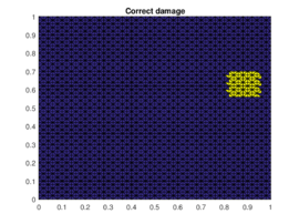
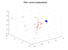
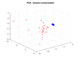
The results of the damaged zone predicted by the proposed method for different positions of the damage are presented in Figures 2 and 3. We can see how it detects quite precisely the position of damaged regions. Moreover in Figure 4 one can see how even if the reduction of dimension performed by the PCA is extreme (only the three first principal components are taken) the zones (damaged and undamaged) are perfectly differentiated.
|
|
(a) |
|

|
(b) |
|
|
(c) |
| Figure 2. Prediction versus reference damage location for the first three different positions of the damaged zone | ||
|
|
| (a) | (c) |
|

|
| (b) | (d) |
| Figure 3. Prediction versus reference damage location for the last two different positions of the damaged zone | |
|
|
| Figure 4. First three principal components of the absolute value of the residual field for case (b) of Figure 2. Red points belong to the damaged zone | |
4. Data completion
The main difficulty when considering the approach discussed above is that the displacement field is needed in as many locations as possible (e.g. the nodes considered in the finite element mesh). Having access to all this local information could become prohibitive in practical applications. Thus, in this section, we consider data acquisition in few locations, from which fields are completed before applying the rationale discussed previously.
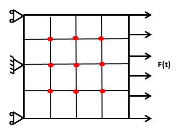
For this purpose a dictionary of simulations is performed, that contains the displacements and residuals fields everywhere for the damage located in different zones and taking different sizes (both perfectly known). In what follows we consider a subdivision of the domain like the one depicted in Figure 5.
|
| Figure 5: Domain division for the dictionary learning. |
We consider 102 scenarios to create our dictionary: the first 48 are given by choosing as damaged zone one of the 16 areas depicted in Figure 5 and assigning to each area 3 different sizes of the damaged zone. The others 54 scenarios are given by choosing as damaged area the 9 intersections of the previous areas (the red points in Figure 5) and assigning to each point 6 possible different sizes of the damaged zone centered on it.
Obviously the dictionary can be enriched with many other locations and sizes of the damaged zone, but the goal in this work is to show how the dictionary learning technique can be used to perform data completion and for this reason the scenarios previously described seem sufficient.
Once the dictionary has been created we suppose that a displacement field related to an unknown damaged scenario is known at few locations, that is, at the positions where sensors are placed. In this work we suppose displacements accessible at the nodes of a uniform grid. It is important to note that coarser dictionaries require much less sensors, whereas rich dictionaries require many measurements in order to identify the closest scenario. In practice we could proceed with coarser representations for online monitoring and richer representations for maintenance operations.
The displacement norms at those locations allow defining matrix , where comes from defined in Eq.(15) by taking the rows corresponding to the sensor points. Then we compute the residual at the sensor points using the same rationale that was considered in Eqs.(16) and (18), but with the difference that now coefficients are obtained in a least-squares sense from
|
|
(19) |
where has been obtained from defined in Eq.(14) by taking the rows corresponding to the sensor points. Let's note that Eq.(19) can be solved because the number of sensor points is greater than the number of functions in the basis (two in the present analysis). Then we reconstruct the damaged displacement norm field at the sensor points by computing
|
|
(20) |
The residual between the reference and the reconstructed damaged displacement norm at the sensor points reads
|
|
(21) |
Then, we compute the gaps between and the residual field at the sensor points of all the simulations in the dictionary, and we select as reference simulation the one that minimizes the norm of this error.
The complete residual field related to the reference simulation is noted by . The reduced base used for data completion is then computed performing a POD on that results in
|
|
(22) |
where is the number of functions selected to compose the reduced base used for the completion.
In order to compute the complete residual field we compute first
|
|
(23) |
where has been obtained from defined in Eq.(22) by taking the rows corresponding to the sensor points and where is smaller than the number of sensors. Thus, it results
|
|
(24) |
As in the previous section the k-means technique is then applied on the absolute value of the completed residual field . Again, in order to reduce the dimensionality of the problem, the PCA is applied on the absolute value of the completed residual field before performing clusterization.
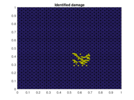
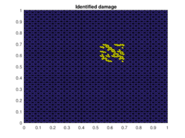
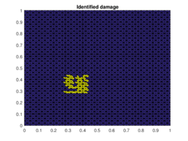
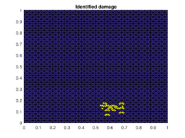
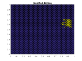
Results on the damaged zone detection by using the proposed methodology for the different positions of the damage considered in the previous section are presented in Figures 6 and 7. We can notice that results are in good agreement to the ones presented in the previous section, with a quite good identification of the damaged zone.

|
|
(a) |

|
|
(b) |

|
|
(c) |
| Figure 6: Results when using data completion for the first three different positions of the damaged zone. | ||

|
|
| (a) | (c) |

|
|
| (b) | (d) |
| Figure 7: Results when using data completion for the last two different positions of the damaged zone. | |
5. Conclusions
In this paper we proposed a new efficient technique for real-time evaluation of damage in structures. For that purpose few POD modes associated with the undamaged structure were used for reconstructing the fields of interest. As expected, as soon as damage occurs, the projection into the undamaged modes allows differentiating using standard clustering techniques, damaged and undamaged regions. Moreover, to avoid data collection on the whole structure, a procedure for collecting data at few specified locations was proposed. Then from the collected data at these points, the fields of interest where completed everywhere, allowing for an accurate damage location.
The numerical test performed proved the validity and potential of the proposed approach thats should be now validated experimentally.
Acknowledgements
The research leading to this works was supported by the ESI group chairs at Centrale Nantes and ENSAM ParisTech and it has received funding from the European Union's Horizon 2020 research and innovation programme under the Marie Sklodowska-Curie grant agreement [675919].
References
[1] Lennart, L., (Ed.) System Identification (2Nd Ed.): Theory for the User. Prentice Hall PTR, 1999.
[2] Peeters, B., De Roeck, G. Stochastic System Identification for Operational Modal Analysis: A Review. ASME. Journal of Dynamic Systems, Measurement and Control, 123(4):659–667, 2001.
[3] Maia, N.M., Silva, J.M.M., Sampaio, R.. Localization of Damage using Curvature of the Frequency-Response-Functions. Proceedings of the 15th International Modal Analysis Conference Society of Experimental Mechanics, Vol. 1, 1997.
[4] Liu, X., Lieven, N., Escamilla-Ambrosio, P.J. Frequency Response Function Shape Based Methods for Structural Damage Localization. Mechanical Systems and Signal Processing, 23:1243–1259, 2009.
[5] Mohan, S.C., Maiti, D.K., Maity, D. Structural damage assessment using FRF employing particle swarm optimization. Applied Mathematics and Computation, 219(20):10387–10400, 2013.
[6] Canales, G., Mevel, L., Basseville, M. Transmissibility based damage detection. SEM. 27th International Modal Analysis Conference (IMAC-XXVII), 2009.
[7] Brincker, R., Zhang, L., Andersen, P. Modal identification of output-only systems using frequency domain decomposition. Smart Materials and Structures, 10(3):441, 2001.
[8] Cawley, P., Adams, R.D. The location of defects in structures from measurements of natural frequencies, IMECHE. The Journal of Strain Analysis for Engineering Design, 14(2):49–57, 1979.
[9] West, W.M. Illustration of the use of modal assurance criterion to detect structural changes in an Orbiter test specimen. Proceedings of the Air Force Conference on Aircraft Structural Integrity, NASA Johnson Space Center, Houston, TX, 3-6 February, 1986.
[10] Salehi, M., Ziaei-Rad, S., Ghayour, M., Ali Vaziri-Zanjani, M., Salehi, M., Ghayour, M., A Vaziri-Zanjani, M. A Structural Damage Detection Technique Based on Measured Frequency Response Functions. Contemporary Engineering Sciences, Vol. 3, 2010.
[11] Pandey, A.K., Biswas, M., Samman, M.M. Damage detection from changes in curvature mode shapes. Journal of Sound and Vibration, 145(2):321–332, 1991.
[12] Yam, L.Y., Leung, T.P., Li, D.B., Xue, K.Z. Theoretical and Experimental Study of Modal Strain Analysis. Journal of Sound and Vibration, 191:251–260, 1996.
[13] Zhang, Z., Aktan, A. The Damage Indices for the Constructed Facilities. Proceedings of the 13th International Modal Analysis Conference, Vol. 2460, 1995.
[14] Xu, W., Cao, M., Ostachowicz, W., Radzieński, M., Xia, N. Two-dimensional curvature mode shape method based on wavelets and Teager energy for damage detection in plates. Journal of Sound and Vibration Supplement, 347(C):266–278, 2015.
[15] Ibrahim, S.R., Mikulcik, E.C. A Method for the Direct Identification of Vibration Parameters from the Free Response. Shock Vib. Bull., 47:183–196, 1977.
[16] Vandiver, J.K., Dunwoody, A.B., Campbell, R.B., Cook, M.F. A Mathematical Basis for the Random Decrement Vibration Signature Analysis Technique. ASME. Journal of Mechanical Design, 104(2):307–313, 1992.
[17] Ibrahim, S.R. Double least squares approach for use in structural modal identification. American Institute of Aeronautics and Astronautics. AIAA Journal, 24(3):499–503,1986.
[18] Juang, J.-N., Pappa, R.S. An eigensystem realization algorithm for modal parameter identification and model reduction. American Institute of Aeronautics and Astronautics. Journal of Guidance, Control, and Dynamics, 8(5):620–627, 1985.
[19] Cattarius, J., Inman, D.J. Time domain analysis for damage detection in smart structures. Mechanical Systems and Signal Processing, 11(3):409–423, 1997.
[20] Ruocci, G., Quattrone, A., De Stefano, A. Multi-domain feature selection aimed at the damage detection of historical bridges. Journal of Physics: Conference Series, 305:012106, 2011.
[21] Park, S.-K., Park, H.W., Shin, S., Lee, H.S. Detection of abrupt structural damage induced by an earthquake using a moving time window technique. Computers & Structures, 86(11):1253–1265, 2008.
[22] Todorovska, M.I., Trifunac, M.D. (2010) Earthquake damage detection in the Imperial County Services Building II: Analysis of novelties via wavelets. Struct. Control Health Monit., 17(8):895–917, 2010.
[23] Todorovska, M.I., Rahmani, M.T. (2013) System identification of buildings by wave travel time analysis and layered shear beam models–Spatial resolution and accuracy. Struct. Control Health Monit., 20(5):686–702, 2013.
[24] Lu, C.-J., Hsu, Y.-T. Vibration analysis of an inhomogeneous string for damage detection by wavelet transform. Int. Journal of Mechanical Sciences, 44(4):745–754, 2002.
[25] Law, S.S., Li, X.Y., Zhu, X.Q., Chan, S.L. Structural damage detection from wavelet packet sensitivity. Engineering Structures, 27(9):1339–1348, 2005.
[26] Xu, Y.L., Chen, J. (2004) Structural Damage Detection Using Empirical Mode Decomposition: Experimental Investigation. Journal of Engineering Mechanics ASCE, 130, 2004.
[27] Ibrahim, S.R., Mikulcik, E.C. (1976) The experimental determination of vibration parameters from time responses. The Shock and Vibration Bulletin, 46(5):187–196, 1976.
[28] James, G., Carne, T., Lauffer, J., Nord, R.A. (1992) Modal testing using natural excitation. Proceedings of the 10th International Modal Analysis Conference, Vol. 2, 1992.
[29] Reynders, E., Teughels, A., De Roeck, G. (2010) Finite element model updating and structural damage identification using OMAX data. Mechanical Systems and Signal Processing, 24(5):1306–1323, 2010.
[30] Huang, Y., Meyer, D., Nemat-Nasser, S. Damage detection with spatially distributed 2D Continuous Wavelet Transform. Mechanics of Materials, 41(10):1096–1107, 2009.
[31] Rucka, M., Wilde, K. (2006) Application of continuous wavelet transform in vibration based damage detection method for beams and plates. Journal of Sound and Vibration, 297(3):536–550, 2006.
[32] Chang, C.-C., Chen, L.-W. (2004) Damage detection of a rectangular plate by spatial wavelet based approach. Applied Acoustics, 65(8):819–832, 2004.
[33] Wang, Q., Deng, X. Damage detection with spatial wavelets. International Journal of Solids and Structures, 36(23):3443–3468, 1999.
[34] Loutridis, S., Douka, E., Trochidis, A. Crack identification in double-cracked beams using wavelet analysis. Journal of Sound and Vibration, 277(4):1025–1039, 2004.
[35] Loutridis, S., Douka, E., Hadjileontiadis, L.J., Trochidis, A. A two-dimensional wavelet transform for detection of cracks in plates. Engineering Structures, 27(9):1327–1338, 2005.
[36] Fan, W., Qiao, P. (2009) A 2-D continuous wavelet transform of mode shape data for damage detection of plate structures. International Journal of Solids and Structures, 46(25):4379–4395, 2009.
[37] Kim, H., Melhem, H. Damage detection of structures by wavelet analysis. Engineering Structures, 26(3):347–362, 2004.
[38] Capellari, G., Eftekhar A.S., Mariani, S. (2015) Damage Detection in Flexible Plates through Reduced-Order Modeling and Hybrid Particle-Kalman Filtering. MDPI. Sensors (Basel, Switzerland), 16(1):2, 2015.
[39] Vitola, J., Vejar, M.A., Burgos, D.A., Pozo, F. Data-Driven Methodologies for Structural Damage Detection Based on Machine Learning Applications. Pattern Recognition - Analysis and Applications. InTech Ch., 06, 2016.
[40] Gui, G., Pan, H., Lin, Z., Li, Y., Yuan, Z. Data-driven support vector machine with optimization techniques for structural health monitoring and damage detection. KSCE Journal of Civil Engineering, 21(2):523–534, 2017.
[41] Taddei, T., Penn, D.J., Yano, M., Patera, A.T. Simulation-Based Classification; a Model-Order-Reduction Approach for Structural Health Monitoring. Archives of Computational Methods in Engineering, 25(1):23-45, 2018.
[42] Mainini, L., Willcox, K. Surrogate Modeling Approach to Support Real-Time Structural Assessment and Decision Making. American Institute of Aeronautics and Astronautics. AIAA Journal, 53(6):1612–1626, 2015.
[43] Muthuraman, U., Sai Hashita, M.M., Sakthieswaran, N., Suresh, P., Uday Raj Kumar, M., Sivashanmugam, P. An Approach for Damage Identification and Optimal Sensor Placement in Structural Health Monitoring by Genetic Algorithm Technique. Circuits and Systems, 7:814–823, 2016.
[44] Gordan, M., Razak, A.H., Ismail, Z., Ghaedi, K. Recent Developments in Damage Identification of Structures Using Data Mining. Latin American Journal of Solids ans Structures, 14(13):2373-2401, 2017.
[45] Selva, P., Cherrier, O., Budinger, V., Lachaud, F., Morlier, J. (2013) Smart monitoring of aeronautical composites plates based on electromechanical impedance measurements and artificial neural networks. Engineering Structures Supplement, 56(C):794–804, 2013.
[46] Lin, N. Monitoring of a Frame Structure Model for Damage Identification using Artificial Neural Networks. 2nd International Conference on Electronic & Mechanical Engineering and Information Technology (EMEIT-2012), Atlantis Press, Paris, France, 2012.
[47] Fish, J., Belytschko, T. A First Course in Finite Elements. John Wiley & Sons, 2007.
[48] Peña, J.M., Lozano, J.A., Larrañaga, P. An empirical comparison of four initialization methods for the K-Means algorithm. Pattern Recognition Letters, 20(10):1027–1040, 1999.
Document information
Published on 08/02/19
Accepted on 09/12/18
Submitted on 09/02/18
Volume 35, Issue 1, 2019
DOI: 10.23967/j.rimni.2018.12.001
Licence: CC BY-NC-SA license
Share this document
claim authorship
Are you one of the authors of this document?