| Line 407: | Line 407: | ||
<div class="center" style="font-size: 75%;">'''Table 1'''. Quadratic errors and approximation order for type I grids</div> | <div class="center" style="font-size: 75%;">'''Table 1'''. Quadratic errors and approximation order for type I grids</div> | ||
| − | <div id=' | + | <div id='table-1'></div> |
{| class="wikitable" style="margin: 1em auto 0.1em auto;border-collapse: collapse;font-size:85%;width:auto;" | {| class="wikitable" style="margin: 1em auto 0.1em auto;border-collapse: collapse;font-size:85%;width:auto;" | ||
|-style="text-align:center" | |-style="text-align:center" | ||
| Line 524: | Line 524: | ||
| 6.3784E-04 | | 6.3784E-04 | ||
| 0.97 | | 0.97 | ||
| − | |||
|} | |} | ||
| − | + | <div class="center" style="font-size: 75%;">'''Table 2'''. Quadratic errors and approximation order for type II grids</div> | |
| − | + | ||
| − | + | <div id='table-2'></div> | |
| − | | <math display="inline">\alpha </math> | + | {| class="wikitable" style="margin: 1em auto 0.1em auto;border-collapse: collapse;font-size:85%;width:auto;" |
| − | + | |-style="text-align:center" | |
| − | + | ! <math display="inline">\alpha </math> !! <math>m</math> !! <math>n</math> !! <math>h</math> | |
| − | + | | <math>\epsilon </math> !! Order | |
| − | | <math>\epsilon </math> | + | |- style="text-align:center" |
| − | + | ||
| − | |- style=" | + | |
| 1.00 | | 1.00 | ||
| 31 | | 31 | ||
| Line 544: | Line 541: | ||
| 0.0064941 | | 0.0064941 | ||
| –– | | –– | ||
| − | |- | + | |-style="text-align:center" |
| 1.00 | | 1.00 | ||
| 71 | | 71 | ||
| Line 551: | Line 548: | ||
| 0.0027556 | | 0.0027556 | ||
| 1.01 | | 1.01 | ||
| − | |- | + | |-style="text-align:center" |
| 1.00 | | 1.00 | ||
| 111 | | 111 | ||
| Line 558: | Line 555: | ||
| 0.0017489 | | 0.0017489 | ||
| 1.01 | | 1.01 | ||
| − | |- | + | |-style="text-align:center" |
| 1.00 | | 1.00 | ||
| 151 | | 151 | ||
| Line 565: | Line 562: | ||
| 0.001281 | | 0.001281 | ||
| 1.00 | | 1.00 | ||
| − | |- | + | |-style="text-align:center" |
| 1.00 | | 1.00 | ||
| 191 | | 191 | ||
| Line 572: | Line 569: | ||
| 0.0010106 | | 0.0010106 | ||
| 1.00 | | 1.00 | ||
| − | |- | + | |-style="text-align:center" |
| 1.00 | | 1.00 | ||
| 231 | | 231 | ||
| Line 579: | Line 576: | ||
| 0.00083446 | | 0.00083446 | ||
| 1.00 | | 1.00 | ||
| − | |- | + | |-style="text-align:center" |
| 1.00 | | 1.00 | ||
| 271 | | 271 | ||
| Line 586: | Line 583: | ||
| 0.0007106 | | 0.0007106 | ||
| 1.00 | | 1.00 | ||
| − | |- | + | |-style="text-align:center" |
| 1.00 | | 1.00 | ||
| 311 | | 311 | ||
| Line 593: | Line 590: | ||
| 0.00061877 | | 0.00061877 | ||
| 1.00 | | 1.00 | ||
| − | |- | + | |-style="text-align:center" |
| 1.25 | | 1.25 | ||
| 31 | | 31 | ||
| Line 600: | Line 597: | ||
| 0.0060306 | | 0.0060306 | ||
| –– | | –– | ||
| − | |- | + | |-style="text-align:center" |
| 1.25 | | 1.25 | ||
| 71 | | 71 | ||
| Line 607: | Line 604: | ||
| 0.0026189 | | 0.0026189 | ||
| 0.99 | | 0.99 | ||
| − | |- | + | |-style="text-align:center" |
| 1.25 | | 1.25 | ||
| 111 | | 111 | ||
| Line 614: | Line 611: | ||
| 0.0016827 | | 0.0016827 | ||
| 0.98 | | 0.98 | ||
| − | |- | + | |-style="text-align:center" |
| 1.25 | | 1.25 | ||
| 151 | | 151 | ||
| Line 621: | Line 618: | ||
| 0.001243 | | 0.001243 | ||
| 0.98 | | 0.98 | ||
| − | |- | + | |-style="text-align:center" |
| 1.25 | | 1.25 | ||
| 191 | | 191 | ||
| Line 628: | Line 625: | ||
| 0.00098714 | | 0.00098714 | ||
| 0.98 | | 0.98 | ||
| − | |- | + | |-style="text-align:center" |
| 1.25 | | 1.25 | ||
| 231 | | 231 | ||
| Line 635: | Line 632: | ||
| 0.00081951 | | 0.00081951 | ||
| 0.97 | | 0.97 | ||
| − | |- | + | |-style="text-align:center" |
| 1.25 | | 1.25 | ||
| 271 | | 271 | ||
| Line 642: | Line 639: | ||
| 0.00070109 | | 0.00070109 | ||
| 0.97 | | 0.97 | ||
| − | |- style=" | + | |- style="text-align:center" |
| 1.25 | | 1.25 | ||
| 311 | | 311 | ||
| Line 649: | Line 646: | ||
| 0.00061294 | | 0.00061294 | ||
| 0.97 | | 0.97 | ||
| − | |||
|} | |} | ||
| − | + | <div class="center" style="font-size: 75%;">'''Table 3'''. Quadratic errors and approximation order for type III grids</div> | |
| − | + | ||
| − | + | <div id='table-2'></div> | |
| − | | <math display="inline">\alpha </math> | + | {| class="wikitable" style="margin: 1em auto 0.1em auto;border-collapse: collapse;font-size:85%;width:auto;" |
| − | + | |-style="text-align:center" | |
| − | + | ! <math display="inline">\alpha </math> !! <math>m</math> !! <math>n</math> !! <math>h</math> | |
| − | + | | <math>\epsilon </math> !! Order | |
| − | | <math>\epsilon </math> | + | |- style="text-align:center" |
| − | + | ||
| − | |- style=" | + | |
| 2.00 | | 2.00 | ||
| 71 | | 71 | ||
| Line 669: | Line 663: | ||
| 9.3949E-04 | | 9.3949E-04 | ||
| 1.77 | | 1.77 | ||
| − | |- | + | |-style="text-align:center" |
| 2.00 | | 2.00 | ||
| 111 | | 111 | ||
| Line 676: | Line 670: | ||
| 4.1865E-04 | | 4.1865E-04 | ||
| 1.80 | | 1.80 | ||
| − | |- | + | |-style="text-align:center" |
| 2.00 | | 2.00 | ||
| 151 | | 151 | ||
| Line 683: | Line 677: | ||
| 2.3926E-04 | | 2.3926E-04 | ||
| 1.81 | | 1.81 | ||
| − | |- | + | |-style="text-align:center" |
| 2.00 | | 2.00 | ||
| 191 | | 191 | ||
| Line 690: | Line 684: | ||
| 1.5584E-04 | | 1.5584E-04 | ||
| 1.82 | | 1.82 | ||
| − | |- | + | |-style="text-align:center" |
| 2.00 | | 2.00 | ||
| 231 | | 231 | ||
| Line 697: | Line 691: | ||
| 1.1006E-04 | | 1.1006E-04 | ||
| 1.82 | | 1.82 | ||
| − | |- | + | |-style="text-align:center" |
| 2.00 | | 2.00 | ||
| 271 | | 271 | ||
| Line 704: | Line 698: | ||
| 8.2131E-05 | | 8.2131E-05 | ||
| 1.83 | | 1.83 | ||
| − | |- | + | |-style="text-align:center" |
| 2.00 | | 2.00 | ||
| 311 | | 311 | ||
| Line 711: | Line 705: | ||
| 6.3786E-05 | | 6.3786E-05 | ||
| 1.83 | | 1.83 | ||
| − | |- | + | |-style="text-align:center" |
| 2.25 | | 2.25 | ||
| 31 | | 31 | ||
| Line 718: | Line 712: | ||
| 4.5265E-03 | | 4.5265E-03 | ||
| –– | | –– | ||
| − | |- | + | |-style="text-align:center" |
| 2.25 | | 2.25 | ||
| 71 | | 71 | ||
| Line 725: | Line 719: | ||
| 9.2020E-04 | | 9.2020E-04 | ||
| 1.91 | | 1.91 | ||
| − | |- | + | |-style="text-align:center" |
| 2.25 | | 2.25 | ||
| 111 | | 111 | ||
| Line 732: | Line 726: | ||
| 3.8741E-04 | | 3.8741E-04 | ||
| 1.93 | | 1.93 | ||
| − | |- | + | |-style="text-align:center" |
| 2.25 | | 2.25 | ||
| 151 | | 151 | ||
| Line 739: | Line 733: | ||
| 2.1315E-04 | | 2.1315E-04 | ||
| 1.94 | | 1.94 | ||
| − | |- | + | |-style="text-align:center" |
| 2.25 | | 2.25 | ||
| 191 | | 191 | ||
| Line 746: | Line 740: | ||
| 1.3496E-04 | | 1.3496E-04 | ||
| 1.94 | | 1.94 | ||
| − | |- | + | |-style="text-align:center" |
| 2.25 | | 2.25 | ||
| 231 | | 231 | ||
| Line 753: | Line 747: | ||
| 9.3190E-05 | | 9.3190E-05 | ||
| 1.94 | | 1.94 | ||
| − | |- | + | |-style="text-align:center" |
| 2.25 | | 2.25 | ||
| 271 | | 271 | ||
| Line 760: | Line 754: | ||
| 6.8259E-05 | | 6.8259E-05 | ||
| 1.95 | | 1.95 | ||
| − | |- | + | |-style="text-align:center" |
| 2.25 | | 2.25 | ||
| 311 | | 311 | ||
| Line 767: | Line 761: | ||
| 5.2179E-05 | | 5.2179E-05 | ||
| 1.95 | | 1.95 | ||
| − | |- | + | |-style="text-align:center" |
| 2.50 | | 2.50 | ||
| 31 | | 31 | ||
| Line 774: | Line 768: | ||
| 4.9361E-03 | | 4.9361E-03 | ||
| –– | | –– | ||
| − | |- | + | |-style="text-align:center" |
| 2.50 | | 2.50 | ||
| 71 | | 71 | ||
| Line 781: | Line 775: | ||
| 9.2007E-04 | | 9.2007E-04 | ||
| 2.02 | | 2.02 | ||
| − | |- | + | |-style="text-align:center" |
| 2.50 | | 2.50 | ||
| 111 | | 111 | ||
| Line 788: | Line 782: | ||
| 3.7194E-04 | | 3.7194E-04 | ||
| 2.02 | | 2.02 | ||
| − | |- | + | |-style="text-align:center" |
| 2.50 | | 2.50 | ||
| 151 | | 151 | ||
| Line 795: | Line 789: | ||
| 1.9951E-04 | | 1.9951E-04 | ||
| 2.02 | | 2.02 | ||
| − | |- | + | |-style="text-align:center" |
| 2.50 | | 2.50 | ||
| 191 | | 191 | ||
| Line 802: | Line 796: | ||
| 1.2407E-04 | | 1.2407E-04 | ||
| 2.02 | | 2.02 | ||
| − | |- | + | |-style="text-align:center" |
| 2.50 | | 2.50 | ||
| 231 | | 231 | ||
| Line 809: | Line 803: | ||
| 8.4506E-05 | | 8.4506E-05 | ||
| 2.02 | | 2.02 | ||
| − | |- | + | |-style="text-align:center" |
| 2.50 | | 2.50 | ||
| 271 | | 271 | ||
| Line 816: | Line 810: | ||
| 6.1224E-05 | | 6.1224E-05 | ||
| 2.02 | | 2.02 | ||
| − | |- | + | |-style="text-align:center" |
| 2.50 | | 2.50 | ||
| 311 | | 311 | ||
| Line 823: | Line 817: | ||
| 4.6380E-05 | | 4.6380E-05 | ||
| 2.02 | | 2.02 | ||
| − | |- | + | |-style="text-align:center" |
| 2.75 | | 2.75 | ||
| 31 | | 31 | ||
| Line 830: | Line 824: | ||
| 5.3606E-03 | | 5.3606E-03 | ||
| –– | | –– | ||
| − | |- | + | |-style="text-align:center" |
| 2.75 | | 2.75 | ||
| 71 | | 71 | ||
| Line 837: | Line 831: | ||
| 9.3491E-04 | | 9.3491E-04 | ||
| 2.10 | | 2.10 | ||
| − | |- | + | |-style="text-align:center" |
| 2.75 | | 2.75 | ||
| 111 | | 111 | ||
| Line 844: | Line 838: | ||
| 3.6799E-04 | | 3.6799E-04 | ||
| 2.08 | | 2.08 | ||
| − | |- | + | |-style="text-align:center" |
| 2.75 | | 2.75 | ||
| 151 | | 151 | ||
| Line 851: | Line 845: | ||
| 1.9446E-04 | | 1.9446E-04 | ||
| 2.07 | | 2.07 | ||
| − | |- | + | |-style="text-align:center" |
| 2.75 | | 2.75 | ||
| 191 | | 191 | ||
| Line 858: | Line 852: | ||
| 1.1975E-04 | | 1.1975E-04 | ||
| 2.06 | | 2.06 | ||
| − | |- | + | |-style="text-align:center" |
| 2.75 | | 2.75 | ||
| 231 | | 231 | ||
| Line 865: | Line 859: | ||
| 8.0998E-05 | | 8.0998E-05 | ||
| 2.06 | | 2.06 | ||
| − | |- | + | |-style="text-align:center" |
| 2.75 | | 2.75 | ||
| 271 | | 271 | ||
| Line 872: | Line 866: | ||
| 5.8375E-05 | | 5.8375E-05 | ||
| 2.05 | | 2.05 | ||
| − | |- | + | |-style="text-align:center" |
| 2.75 | | 2.75 | ||
| 311 | | 311 | ||
| Line 879: | Line 873: | ||
| 4.4042E-05 | | 4.4042E-05 | ||
| 2.05 | | 2.05 | ||
| − | |- | + | |-style="text-align:center" |
| 3.00 | | 3.00 | ||
| 31 | | 31 | ||
| Line 886: | Line 880: | ||
| 5.7955E-03 | | 5.7955E-03 | ||
| –– | | –– | ||
| − | |- | + | |-style="text-align:center" |
| 3.00 | | 3.00 | ||
| 71 | | 71 | ||
| Line 893: | Line 887: | ||
| 9.6029E-04 | | 9.6029E-04 | ||
| 2.17 | | 2.17 | ||
| − | |- | + | |-style="text-align:center" |
| 3.00 | | 3.00 | ||
| 111 | | 111 | ||
| Line 900: | Line 894: | ||
| 3.7142E-04 | | 3.7142E-04 | ||
| 2.13 | | 2.13 | ||
| − | |- | + | |-style="text-align:center" |
| 3.00 | | 3.00 | ||
| 151 | | 151 | ||
| Line 907: | Line 901: | ||
| 1.9454E-04 | | 1.9454E-04 | ||
| 2.10 | | 2.10 | ||
| − | |- | + | |-style="text-align:center" |
| 3.00 | | 3.00 | ||
| 191 | | 191 | ||
| Line 914: | Line 908: | ||
| 1.1915E-04 | | 1.1915E-04 | ||
| 2.09 | | 2.09 | ||
| − | |- | + | |-style="text-align:center" |
| 3.00 | | 3.00 | ||
| 231 | | 231 | ||
| Line 921: | Line 915: | ||
| 8.0299E-05 | | 8.0299E-05 | ||
| 2.08 | | 2.08 | ||
| − | |- | + | |-style="text-align:center" |
| 3.00 | | 3.00 | ||
| 271 | | 271 | ||
| Line 928: | Line 922: | ||
| 5.7715E-05 | | 5.7715E-05 | ||
| 2.07 | | 2.07 | ||
| − | |- style=" | + | |- style="text-align:center" |
| 3.00 | | 3.00 | ||
| 311 | | 311 | ||
| Line 935: | Line 929: | ||
| 4.3453E-05 | | 4.3453E-05 | ||
| 2.06 | | 2.06 | ||
| − | |||
|} | |} | ||
Revision as of 14:13, 13 January 2021
Abstract
In this paper, it is presented a formulation of a generalized finite difference scheme to solve the Motz problem. It is based on a general difference scheme defined by an optimality condition, which has been developed to solve Poisson-like equations whose domains are approximated by a wide variety of grids over general regions. Numerical examples showing second-order accuracy of the calculated solutions are presented.
Keywords: Generalized finite difference, Motz problem
1. The Motz problem
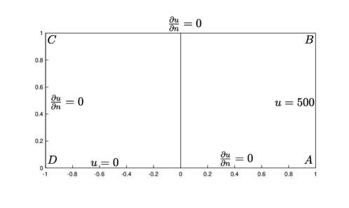
The Motz problem is a benchmark for the Laplace equation problem that is often used for testing various special numerical methods; it was proposed in the literature for the solution of elliptic boundary value problems with boundary singularities. The boundary value problem is stated as follows (Figure 1)
|
|
A singularity similar to that at the origin appears analogously in several hydrological applications, often related to an abrupt change in the boundary condition, particularly in groundwater infiltration in the alternation of pervious and impervious boundary zones.
|
| Figure 1. Motz problem domain and boundary conditions |
The closed-form solution of Motz problem is given as a series
|
|
(1) |
where and are the polar coordinates; its convergence ratio is 2, and therefore valid over the whole domain (Figure 1).
Several papers discuss the accurate numerical calculation of the coefficients . Lu [1] calculated them with 17 significant digits using a collocation Treftz method. Li et al. [2] used a special boundary approximation method to derive the leading coefficients of the asymptotic solution expansion. Similar approaches were followed by Li et al. [3] and Arad et al. [4], who employed boundary methods combined with least-squares and penalty method techniques to handle the boundary information, and by Georgiou [5], who employed Lagrange multipliers.
Some other authors focus on solving the Motz problem using different numerical techniques. Bernal and Kindelan [6] thoroughly discussed the performance of the radial basis function method in the solution of the Motz problem, including the global radial basis function method due to Kansa [7], as well as Shu's local differential quadrature method based on radial basis functions [8]. They showed that the exponential convergence obtained by increasing resolution and increasing the shape parameter is lost due to the presence of the singularity. The accuracy of the solution can be increased by using collocation at some boundary nodes to restore the convergence of the method, although it is necessary to use functions similar to the terms in equation (1), which are capable of capturing the behaviour of the solution near the discontinuity.
To produce an accurate solution based on the flexibility of meshfree methods, Hong [9] addressed a singular basis function enrichment technique in a meshless method, using the leading terms of the local series expansion at the boundary singularity, as enrichment functions for a local approximation space constructed to calculate the solution. The enrichment technique is derived from the Generalized Finite Element Method (GFEM) and produces accurate results, although it requires smooth global support basis functions and basis enrichment to produce the numerical solution.
The aforementioned papers give an insight into the different approaches considered in the problem. Finite elements and radial basis functions can be certainly used to produce accurate results near the singularity, although it is also possible to consider the little restrictive and more versatile alternative given by the Generalized Finite Differences Method (GFDM), which has recently been used to produce satisfactory approximations to solve differential equations in a wide number of applications modeled over irregular regions; for instance, on structured grids, a Generalized Crank Nicolson scheme is presented in [10]. Chávez et al showed a stable calculation of the solution of nonlinear Richards equation which avoids oscillations in high gradient regions in [11], and Tinoco et al addressed the conditions for stability in general schemes in [12].
The GFDM is not limited to a grid structure, and can also be applied on unstructured grids and even as a meshless method in clouds of points: Benito et al studied its use on parabolic and hyperbolic equations [13], advection-diffusion equations [14], seismic wave problems [15] and nonlinear elliptic equations [16] . Fan et al have applied general finite differences on Burgers equation [17], obstacle problems [18], shallow water equations [19] and natural double convection problems [20].
In this paper, bearing in mind the engineering applications where the use of GFDM has been successfully applied, this paper shows an accurate numerical approximation to the solution of Motz problem.
It is organized as follows: generalized finite differences are presented in Section 2. The description of the meshes used is given in Section 3. Numerical tests are described in Section 4; discussion and conclusions in Section 5, followed by conclusions in Section 6.
2. General finite differences
A very common and widely used discretization procedure to approximate the solutions of differential equations is the finite difference method. This is because it can be easily applied in block-rectangular regions.
The well-known classic schemes for the first and second-order derivatives can be easily deduced from basic analytical considerations or by straightforward application of the Taylor theorem. Despite the basic idea of the theorem is quite simple, its use leads to more complicated schemes on non-rectangular regions when the geometry associated with the scheme changes. Nevertheless, when symmetry is involved, very interesting approaches can be considered; like those due to Liszka [21] for regular hexagonal geometries and to Benito [22,13] for slightly perturbed clouds of nodes.
In the following paragraphs, we discuss the use of a general difference scheme that can be calculated by considering a set of nodes where the solution of a differential equation is evaluated or approximated. For these nodes it is required to find coefficients in such a way that consistency condition is fulfilled. In other words, the local truncation error to approximate the second-order linear operator
|
|
(2) |
at the grid point employing the combination
|
|
(3) |
must satisfy the condition
|
|
(4) |
as [23].
The coefficients may change from one inner grid point to another in an irregular region, since they depend on the positions of the nodes relative to . Nevertheless, in the case of nearly rectangular grids and the Laplace equation, since the coefficients are invariant under rotations and translations, essentially one set of coefficients is required.
For the sake of brevity, in the following paragraphs the coefficient
|
|
will be denoted as .
Let and be the and components of , respectively. Thus, the local truncation error (up to second-order) yields
|
|
Therefore, assuming smoothness of , to get second-order local consistency the coefficients of the derivatives of at the right-hand side of the expansion must satisfy the linear system
|
|
(5) |
One must note that, in general, this system is not well-determined. This poses the calculation of the coefficients in terms of a well studied algebraic problem which can be solved robustly. Hence, the main question is how to produce a solution of equation (5) which provides a consistent second-order scheme. Several alternatives are possible, for example, in [10], an efficient heuristic calculation to solve numerically the diffusion equation was proposed. It was based on an unconstrained optimization problem for every inner grid point. To apply it, first, we separate the first equation of the matrix system (5)
|
|
(6) |
and then we solve the system
|
|
(7) |
where
|
|
(8) |
|
|
(9) |
Next, is obtained from equation (6).
Equation (7) defines the generalized finite differences in general grids. To solve it is straightforward when the grid is rectangular or nearly rectangular, and a sufficient number of nodes or symmetries are available.
In irregular grids or clouds of points, which lack symmetry, the system defined by is underdetermined if , which means that, in that case, at least seven neighbor nodes around are required to get local consistency.
On the other hand, in a rather regular structured -or mapping- grid, symmetries reduce the number of required neighbors. An important consequence is that the symmetric location of nodes around the central node avoids rank deficiency of in the system (7).
3. Grids and stencils
The main issue to consider when solving the Motz problem is the singularity in the partial derivative at the origin of coordinates. The usual approach to produce an accurate approximation at that point is to refine the grid around it. However, this causes not only an increase in the computational cost, but often the results are not satisfactory due to the high gradient values of the solution on the positive -axis; even with robust techniques as those based on radial basis functions [6], a special treatment is required near the origin. Some other approaches, like that of Hong, require a rather sophisticated process of patch mapping to produce accurate results [9].
When finite differences are considered, it is important to emphasize that the method has been successfully applied to problems with strong boundary layers, for instance, by Ivanenko [24] and Pereyra [25], when the equidistribution principle is addressed. In other words, the key is to produce a suitably adapted grid through a simple procedure. In this paper, to derive the rule that controls the refinement around the origin, the clue is given by the shape of the significative terms in the closed-form solution series of equation (1).
Bearing in mind the equidistribution principle as discussed by Ivanenko, since the graph of the solution is monotonic along the positive -axis, and resembles that of a boundary layer, there is a mapping such that the expression
|
|
(10) |
is constant. According to eq. (1), each term in the solution along such axis equals , . Therefore, the constant right-hand side of (10) takes the form
|
|
This implies that the partial derivative must have the form and, in consequence, the grid refinement is of the form
|
|
(11) |
According to the estimations presented by Lu [1], the first five coefficients in the equation (1) are the significative ones: Those terms correspond to . Since the value in equation (11) represents an increase in the distance between the grid nodes around the origin, only the value , which corresponds to , is considered.
Thus, the mesh adaptation procedure is as follows:
- The grid for the whole domain of the problem is generated in the first step as a regular rectangular grid.
- Every cell is subdivided into two triangles in the second step to define six neighbours in the stencil for every inner grid node.
- Finally, the grid is adapted by modifying the grid coordinates following the mapping given by equation(11).
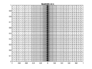
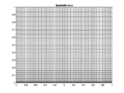
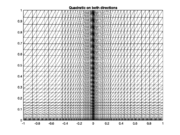
In the numerical tests, the interval was considered for the exponent . For comparison purposes, the mapping was applied to the -axis (Type I grids), to the -axis (Type II grids), and both axes (Type III). An example of the grids corresponding to the different distributions is shown in Figure 2.
|
|
|
| Figure 2. Examples of the kinds of grids used in the tests | ||
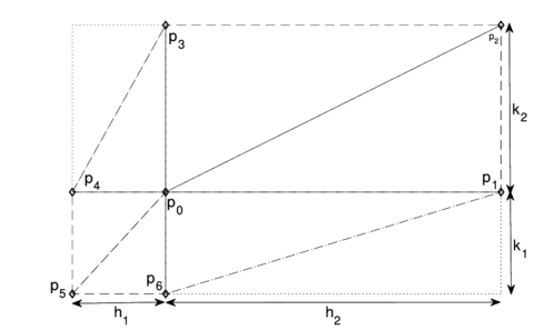
The three kinds of grids define a regular location of neighbors at the inner nodes: star-shaped subgrids with 6 neighbours that can be used to approximate the derivatives in the left-hand side of equation (6); an example of such subgrid can be seen in Figure 3. The Laplacian operator is approximated at the point , and the corresponding neighbours are , , , , , and . The values , , , and are the step size lengths in the stencil. Bearing in mind equation (5), this poses a problem with 6 equations and unknowns; since the values , , , and are non zero, after preconditioning of equation (6) by scaling, the rank of is equal to five, which allows a robust calculation of the coefficients and leaves one degree of freedom available.
|
| Figure 3. Selection of neighbours for an inner grid node |
Regarding the boundary condition, a straightforward discretization using the GFDM method was addressed in [26]: at a boundary node of a structured grid, equation (7) is evaluated at its five neighbors, taking the right-hand side to define the directional derivative. However, since the neighbors are often not balanced around the boundary node, such selection might produce first approximations which could cause loss of order in the Motz problem with the grids considered here.
In this paper, we define an ad hoc ghost point to avoid loss of accuracy. The boundary condition
|
|
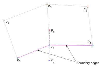
where is the outer normal vector at , is approximated using the scheme of equation (5) with and , using 7 points: a ghost point , and the nodes , , , , and (Figure 4), which yields the equation (12)
|
|
(12) |
or, in other words,
|
|
(13) |
For convenience, the ghost point is calculated in such a way that is the midpoint of and , the latter being the centroid of the nodes , , , , , and (Figure 4).
The value of given by the equation (13) is substituted in the approximation to the Laplacian (equation (7) at using the same 7 points , , , , , , and , which eliminates the value of .
Te assembled system for the whole grid becomes sparse as the number of grid points per side increases; it was solved using a sparse lu decomposition to produces the approximation to the solution of the problem.
|
| Figure 4. Selection of ghost point at a boundary node of a general structured grid with Neumann condition |
4 Numerical tests
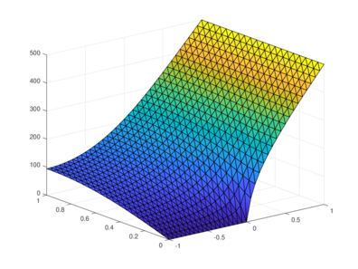
Several tests were performed with and nodes per side on the and directions, respectively, varying from 31 to 351. Grids of the three types in the previous section were generated, and the Motz problem was solved using the proposed scheme for every grid size and distribution. An example of the finite difference discretization described in the previous section is sketched in Figure 5.
|
| Figure 5. Grid and calculated solution |
To assess the accuracy of the numerical solution, since the approximation was calculated using structured grids, the quadratic error
|
|
(14) |
was used, where is the solution calculated using the difference scheme at the point , is the exact solution (equation (1)) at the same point, and is the area of the rhombus defined by the nodes .
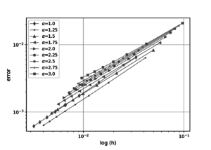
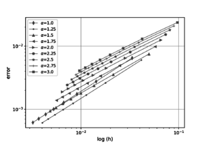
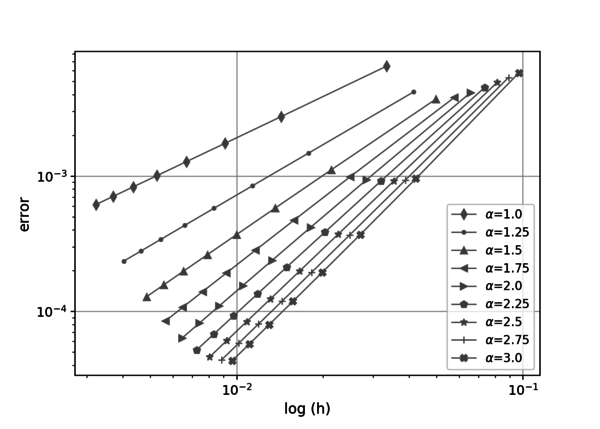
The measure of the roughness of the grid is given by the meh norm ; the log graph of the mean square errors versus the grid norm for the type I and II grids are shown in Figures 6 and 7. One can note that there is a clear convergence tendency on all the tests despite the boundary singularity. But, when only a nonuniform distribution either along the or the -axis is used, the second-order approximation is lost, in a similar way as reported by Bernal using radial basis functions. The best results are obtained with the grids which are non-uniform on and , as can be seen in Figure 7.
|
|
| Figure 6. Log values of the quadratic errors, nonuniform node distribution on or | |
|
| Figure 7. Log values of the quadratic errors, nonuniform node distribution on and |
The values of the errors, grid norms, and estimated convergence order are shown in Tables 1 to 3. The values in the last table show that, indeed, quadratic convergence is obtained when the same nonuniform node distribution along both axes is used, even in the presence of the boundary singularity.
| !! Order | |||||
| 1.00 | 31 | 61 | 3.3333E-02 | 6.4941E-03 | –– |
| 1.00 | 71 | 141 | 1.4286E-02 | 2.7556E-03 | 1.01 |
| 1.00 | 111 | 221 | 9.0909E-03 | 1.7489E-03 | 1.01 |
| 1.00 | 151 | 301 | 6.6667E-03 | 1.2810E-03 | 1.00 |
| 1.00 | 191 | 381 | 5.2632E-03 | 1.0106E-03 | 1.00 |
| 1.00 | 231 | 461 | 4.3478E-03 | 8.3446E-04 | 1.00 |
| 1.00 | 271 | 541 | 3.7037E-03 | 7.1060E-04 | 1.00 |
| 1.00 | 311 | 621 | 3.2258E-03 | 6.1877E-04 | 1.00 |
| 1.25 | 31 | 61 | 4.1492E-02 | 6.4057E-03 | –– |
| 1.25 | 71 | 141 | 1.7825E-02 | 2.7333E-03 | 1.01 |
| 1.25 | 111 | 221 | 1.1351E-02 | 1.7503E-03 | 0.99 |
| 1.25 | 151 | 301 | 8.3264E-03 | 1.2920E-03 | 0.98 |
| 1.25 | 191 | 381 | 6.5746E-03 | 1.0260E-03 | 0.98 |
| 1.25 | 231 | 461 | 5.4318E-03 | 8.5207E-04 | 0.97 |
| 1.25 | 271 | 541 | 4.6275E-03 | 7.2925E-04 | 0.97 |
| 1.25 | 311 | 621 | 4.0306E-03 | 6.3784E-04 | 0.97 |
| !! Order | |||||
| 1.00 | 31 | 61 | 0.033333 | 0.0064941 | –– |
| 1.00 | 71 | 141 | 0.014286 | 0.0027556 | 1.01 |
| 1.00 | 111 | 221 | 0.0090909 | 0.0017489 | 1.01 |
| 1.00 | 151 | 301 | 0.0066667 | 0.001281 | 1.00 |
| 1.00 | 191 | 381 | 0.0052632 | 0.0010106 | 1.00 |
| 1.00 | 231 | 461 | 0.0043478 | 0.00083446 | 1.00 |
| 1.00 | 271 | 541 | 0.0037037 | 0.0007106 | 1.00 |
| 1.00 | 311 | 621 | 0.0032258 | 0.00061877 | 1.00 |
| 1.25 | 31 | 61 | 0.041492 | 0.0060306 | –– |
| 1.25 | 71 | 141 | 0.017825 | 0.0026189 | 0.99 |
| 1.25 | 111 | 221 | 0.011351 | 0.0016827 | 0.98 |
| 1.25 | 151 | 301 | 0.0083264 | 0.001243 | 0.98 |
| 1.25 | 191 | 381 | 0.0065746 | 0.00098714 | 0.98 |
| 1.25 | 231 | 461 | 0.0054318 | 0.00081951 | 0.97 |
| 1.25 | 271 | 541 | 0.0046275 | 0.00070109 | 0.97 |
| 1.25 | 311 | 621 | 0.0040306 | 0.00061294 | 0.97 |
| !! Order | |||||
| 2.00 | 71 | 141 | 2.8367E-02 | 9.3949E-04 | 1.77 |
| 2.00 | 111 | 221 | 1.8099E-02 | 4.1865E-04 | 1.80 |
| 2.00 | 151 | 301 | 1.3289E-02 | 2.3926E-04 | 1.81 |
| 2.00 | 191 | 381 | 1.0499E-02 | 1.5584E-04 | 1.82 |
| 2.00 | 231 | 461 | 8.6767E-03 | 1.1006E-04 | 1.82 |
| 2.00 | 271 | 541 | 7.3937E-03 | 8.2131E-05 | 1.83 |
| 2.00 | 311 | 621 | 6.4412E-03 | 6.3786E-05 | 1.83 |
| 2.25 | 31 | 61 | 7.3442E-02 | 4.5265E-03 | –– |
| 2.25 | 71 | 141 | 3.1856E-02 | 9.2020E-04 | 1.91 |
| 2.25 | 111 | 221 | 2.0338E-02 | 3.8741E-04 | 1.93 |
| 2.25 | 151 | 301 | 1.4938E-02 | 2.1315E-04 | 1.94 |
| 2.25 | 191 | 381 | 1.1803E-02 | 1.3496E-04 | 1.94 |
| 2.25 | 231 | 461 | 9.7560E-03 | 9.3190E-05 | 1.94 |
| 2.25 | 271 | 541 | 8.3140E-03 | 6.8259E-05 | 1.95 |
| 2.25 | 311 | 621 | 7.2434E-03 | 5.2179E-05 | 1.95 |
| 2.50 | 31 | 61 | 8.1262E-02 | 4.9361E-03 | –– |
| 2.50 | 71 | 141 | 3.5333E-02 | 9.2007E-04 | 2.02 |
| 2.50 | 111 | 221 | 2.2573E-02 | 3.7194E-04 | 2.02 |
| 2.50 | 151 | 301 | 1.6583E-02 | 1.9951E-04 | 2.02 |
| 2.50 | 191 | 381 | 1.3106E-02 | 1.2407E-04 | 2.02 |
| 2.50 | 231 | 461 | 1.0834E-02 | 8.4506E-05 | 2.02 |
| 2.50 | 271 | 541 | 9.2336E-03 | 6.1224E-05 | 2.02 |
| 2.50 | 311 | 621 | 8.0450E-03 | 4.6380E-05 | 2.02 |
| 2.75 | 31 | 61 | 8.9015E-02 | 5.3606E-03 | –– |
| 2.75 | 71 | 141 | 3.8796E-02 | 9.3491E-04 | 2.10 |
| 2.75 | 111 | 221 | 2.4802E-02 | 3.6799E-04 | 2.08 |
| 2.75 | 151 | 301 | 1.8227E-02 | 1.9446E-04 | 2.07 |
| 2.75 | 191 | 381 | 1.4407E-02 | 1.1975E-04 | 2.06 |
| 2.75 | 231 | 461 | 1.1911E-02 | 8.0998E-05 | 2.06 |
| 2.75 | 271 | 541 | 1.0152E-02 | 5.8375E-05 | 2.05 |
| 2.75 | 311 | 621 | 8.8459E-03 | 4.4042E-05 | 2.05 |
| 3.00 | 31 | 61 | 9.6704E-02 | 5.7955E-03 | –– |
| 3.00 | 71 | 141 | 4.2248E-02 | 9.6029E-04 | 2.17 |
| 3.00 | 111 | 221 | 2.7026E-02 | 3.7142E-04 | 2.13 |
| 3.00 | 151 | 301 | 1.9867E-02 | 1.9454E-04 | 2.10 |
| 3.00 | 191 | 381 | 1.5707E-02 | 1.1915E-04 | 2.09 |
| 3.00 | 231 | 461 | 1.2987E-02 | 8.0299E-05 | 2.08 |
| 3.00 | 271 | 541 | 1.1070E-02 | 5.7715E-05 | 2.07 |
| 3.00 | 311 | 621 | 9.6462E-03 | 4.3453E-05 | 2.06 |
5 Results and discussion
Several assertions can be drawn from the numerical results. First, despite the presence of the boundary singularity, the results are accurate enough. This is certainly a strength of the proposed finite difference scheme, which is rather simple. Since the main differences between the scheme discussed in this paper and the standard five-point scheme for the Laplacian are the addition of two extra “diagonal” nodes in the inner grid nodes and the use of a suitable grid spacing, this suggests that the proposed stencils are suitable to produce accurate results.
The convergence orders in table 3 must be highlighted. Having in mind the presence of the singularity and the simplicity of the addressed difference stencils, this is indeed a remarkable result. Since the boundary node redistribution was defined by a very simple rule, this suggests that it is unnecessary to consider another kind of grids or more complex refinements near the singularity to solve the Motz problem, although, it must be acknowledged that the mesh adapting strategy was proposed ad hoc for it. Naturally, the numerical treatment of different singularities in other problems require a different application of the equidistribution principle.
6 Conclusions
Indeed, generalized finite differences can be used to solve the Motz problem numerically. The numerical results show that generalized finite differences produce accurate solutions to a complicated benchmark problem, and the most noteworthy fact is that this can be done even with very simple structured grids. This is an important feature of the GFDM method, considering the difficulty of the problem. Thinking about the solution to several linear and nonlinear problems with this method which appear in the literature [27,10,22,13], it is certainly a reliable numerical tool.
The results are very encouraging since boundary configurations similar to those of Motz problem appear in several relevant applications, for instance, in interfaces between different media in infiltration problems, or advection-diffusion problems with sources and sinks along the boundary. Both problems are currently under investigation and advances in this sense will be reported in a future paper.
Acknowledgments
We want to thank CIC-UMSNH 9.16, and Aula-CIMNE Morelia for the financial support for this work.
BIBLIOGRAPHY
[1] Lu, T. T. and Hu, H. Y. and Li, Z. C. (2004) "Highly accurate solutions of Motz's and the cracked beam problems", Volume 28. Engineering Analysis with Boundary Elements 1387–1403
[2] Li, Z. C. and Mathon, R. and Sermer, P. (1987) "Boundary methods for solving elliptic problems with singularities and interfaces", Volume 24. SIAM Journal of Numerical Analaysis 487–498
[3] Li, Z. C. and Mathon, R. and Sermer, P. (1987) "Boundary methods for solving elliptic problems with singularities and interfaces", Volume 24. SIAM Journal on Numerical Analysis 3 487-498
[4] Yosibash, Z. and Ben-Dor, G. and Yakhot, A. (1998) "Computing flux intensity factors by a boundary method for elliptic equations with singularities", Volume 14. Communications in Numerical Methods in Engineering 657–670
[5] Georgiou, G. C. and Olson, L. and Smyrlis, Y. S. (1996) "A singular function boundary integral method for the laplace equation", Volume 12. Communications in Numerical Methods in Engineering 2 127-134
[6] Bernal, Francisco and Kindelan, Manuel. (2010) "Radial basis function solution of the Motz problem", Volume 27. Engineering Computations 606–620
[7] Kansa, E. J. (1990) "Multiquadrics, a scattered data approximation scheme with applications to computational fluid dynamics II: solutions to parabolic, hyperbolic and elliptic partial differential equations", Volume 19. Computers and Mathematics with Applications 147–161
[8] Shu, C. and Ding, H. and Yeo, K. S. (2003) "Local radial basis function-based differential quadrature method and its application to solve two-dimensional incompressible Navier-Stokes equations", Volume 192. Computer Methods in Applied Mechanics and Engineering 3 941–954
[9] Hong, Won-Tak. (2016) "Enriched Meshfree Method for an Accurate Numerical Solution of the Motz Problem"
[10] Domínguez-Mota, F. J. and Armenta, S. M. and Tinoco-Guerrero, G. and Tinoco-Ruiz, J. G. (2014) "Finite difference schemes satisfying an optimality condition for the unsteady heat equation", Volume 106. Mathematics and Computers in Simulation 76–83
[11] Chávez-Negrete, C and Domínguez-M, F and Santana-Quinteros, D. (2018) "Numerical solution of Richards' equation of water flow by generalized finite differences", Volume 101. Computers and Geotechnics 1 168–175
[12] Tinoco-Guerrero, G. and Domínguez-Mota, F. J. and Gaona-Arias, A. and Ruiz-Zavala, M. L. and Tinoco-Ruiz, J. G. (2018) "A stability analysis for a generalized finite-difference scheme applied to the pure advection equation", Volume 147. Mathematics and Computers in Simulation 293–300
[13] Muñoz, J. J. B. and Ureña-Prieto, F. and Corvinos, L. A. G. (2007) "Solving parabolic and hyperbolic equations by the generalized finite difference method", Volume 209. Journal of Computational and Applied Mathematics 2 208–233
[14] Ureña, F. and Benito, J. J. and Gavete, L. (2011) "Application of the generalized finite difference method to solve the advection-diffusion equation", Volume 235. Journal of Computational and Applied Mathematics 1849–1855
[15] Ureña, F. and Benito, J. J. and Salete, E. and Gavete, L. (2012) "A note on the application of the generalized finite difference method to seismic wave propagation in 2D", Volume 236. Journal of Computational and Applied Mathematics 3016–3025
[16] Muñoz, J. J. B. and Ureña-Prieto, F. and Corvinos, L. and Gavete, A. (2017) "Solving second order non-linear elliptic partial differential equations using generalized finite difference method", Volume 318. Journal of Computational and Applied Mathematics 378–387
[17] Chan, Hsin-Fang and Wei Li, Po. (2013) "Generalized finite difference method for solving two-dimensional Burgers' equations", Volume 79. Procedia Engineering 55–60
[18] Chan, Hsin-Fang and Ming Fan, Chia and Kuo, Chia-Wen. (2013) "Generalized finite difference method for solving two-dimensional non-linear obstacle problem", Volume 37. Engineering Analysis with Boundary Elements 1189–1196
[19] Wei Li, Po and Ming Fan, Chia. (2017) "Generalized finite difference method for two-dimensional shallow water equations", Volume 80. Engineering Analysis with Boundary Elements 58–71
[20] Chan, Hsin-Fang and Ming Fan, Chia and Kuo, Chia-Wen. (2018) "Generalized finite difference method for solving the double-diffusive natural convection in fluid-saturated porous media", Volume 95. Engineering Analysis with Boundary Elements 175–186
[21] Liszka, T. and Orkisz, J. (1980) "The finite difference method at arbitrary irregular grids and its application in applied mechanics", Volume 11. Computers and Structures 1 83–95
[22] Muñoz, J. J. B. and Prieto, J. B. and Corvinos, L. A. G. and Alonso, B. (2008) "A posteriori error estimator and indicator in generalized finite differences. Application to improve the approximated solution of elliptic pde's.", Volume 85. International Journal of Computer Mathematics 3-4 359–370
[23] Celia, M. and Gray, W. (1992) "Numerical Methods for Differential Equations". Prentice-Hall
[24] Ivanenko, S. (2003) "Selected chapters on grid generation and applications. Azarenok, B. (Ed.)". Russian academy of sciences
[25] Pereyra, V. and Sewell, G. (1975) "A singular function boundary integral method for the laplace equation", Volume 23. Numer. Math. 261-268
[26] Francisco-Javier Domínguez-Mota and Sanzon Mendoza-Armenta and José-Gerardo Tinoco-Ruiz and Gerardo Tinoco-Guerrero. (2011) "Numerical Solution of Poisson-like Equations with Robin Boundary Conditions Using a Finite Difference Scheme Dfined by an Optimality Condition", Volume 17. MASCOT11 Proceedings 101-110
[27] Domínguez-M, F. J. and Equihua, M. and Mendoza, S. and Tinoco-R., J. G. (2010) "Solución de ecuaciones diferenciales elípticas en regiones planas irregulares usando mallas convexas generadas por métodos variacionales empleando elementos finitos", Volume 26. Rev. Int. Mét. Num. Cálc. Dis. Ing. 187–194
Document information
Published on 14/01/21
Accepted on 02/01/21
Submitted on 12/04/20
Volume 37, Issue 1, 2021
DOI: 10.23967/j.rimni.2021.01.004
Licence: CC BY-NC-SA license