Danielquer (talk | contribs) m (Danielquer moved page Review Radulescu 2018b to Radulescu 2018a) |
|||
| (2 intermediate revisions by one other user not shown) | |||
| Line 81: | Line 81: | ||
As regards the Cobb-Douglas production function it is expressed in the following relation: | As regards the Cobb-Douglas production function it is expressed in the following relation: | ||
| − | '''Y = L<sup>α</sup> x K <sup>1-α</sup> x TFP | + | {| class="formulaSCP" style="width: 100%; text-align: left;" |
| + | |- | ||
| + | | | ||
| + | {| style="text-align: center; margin:auto;width: 100%;" | ||
| + | |- | ||
| + | | style="text-align: center;" | '''Y = L<sup>α</sup> x K <sup>1-α</sup> x TFP''' | ||
| + | | style="width: 5px;text-align: right;white-space: nowrap;" |(1.1) | ||
| + | |} | ||
| + | |} | ||
where Y, L, K, TFP and α represent the GDP, the labour factor, the capital stock, the total factor productivity and the output elasticity of labour. | where Y, L, K, TFP and α represent the GDP, the labour factor, the capital stock, the total factor productivity and the output elasticity of labour. | ||
| Line 87: | Line 95: | ||
By applying logarithms the relation (1.1) turns into: | By applying logarithms the relation (1.1) turns into: | ||
| − | '''Y<sub>t</sub> = α x L<sub>t</sub> + (1 - α) x K<sub>t</sub> + TFP<sub>t</sub>, | + | {| class="formulaSCP" style="width: 100%; text-align: left;" |
| + | |- | ||
| + | | | ||
| + | {| style="text-align: center; margin:auto;width: 100%;" | ||
| + | |- | ||
| + | | style="text-align: center;" | '''Y<sub>t</sub> = α x L<sub>t</sub> + (1 - α) x K<sub>t</sub> + TFP<sub>t</sub>,''' | ||
| + | | style="width: 5px;text-align: right;white-space: nowrap;" |(1.2) | ||
| + | |} | ||
| + | |} | ||
where Y'''<sub>t</sub>''', L'''<sub>t</sub>''', K'''<sub>t</sub>''' and TFP'''<sub>t</sub>''' are the YoY paces for GDP, labour factor, capital stock and the total factor productivity. | where Y'''<sub>t</sub>''', L'''<sub>t</sub>''', K'''<sub>t</sub>''' and TFP'''<sub>t</sub>''' are the YoY paces for GDP, labour factor, capital stock and the total factor productivity. | ||
| Line 95: | Line 111: | ||
The dynamics of the potential GDP can be expressed as in the following relation: | The dynamics of the potential GDP can be expressed as in the following relation: | ||
| − | '''Y<sub>t</sub>* = α x L<sub>t</sub>* + (1 - α) x K<sub>t</sub> + TFP<sub>t</sub>*, | + | {| class="formulaSCP" style="width: 100%; text-align: left;" |
| + | |- | ||
| + | | | ||
| + | {| style="text-align: center; margin:auto;width: 100%;" | ||
| + | |- | ||
| + | | style="text-align: center;" | '''Y<sub>t</sub>* = α x L<sub>t</sub>* + (1 - α) x K<sub>t</sub> + TFP<sub>t</sub>*,''' | ||
| + | | style="width: 5px;text-align: right;white-space: nowrap;" |(1.3) | ||
| + | |} | ||
| + | |} | ||
where Y<sub>t</sub>*, L<sub>t</sub>* and TFP<sub>t</sub>* represent the trend component for the dynamics of the GDP, labour factor and total factor productivity. | where Y<sub>t</sub>*, L<sub>t</sub>* and TFP<sub>t</sub>* represent the trend component for the dynamics of the GDP, labour factor and total factor productivity. | ||
| Line 101: | Line 125: | ||
The labour factor (L) was defined as: | The labour factor (L) was defined as: | ||
| − | '''L = labour force x labour participation ratio x (1-unemployment rate) x number of the worked hours | + | {| class="formulaSCP" style="width: 100%; text-align: left;" |
| + | |- | ||
| + | | | ||
| + | {| style="text-align: center; margin:auto;width: 100%;" | ||
| + | |- | ||
| + | | style="text-align: center;" | '''L = labour force x labour participation ratio x (1-unemployment rate) x number of the worked hours''' | ||
| + | | style="width: 5px;text-align: right;white-space: nowrap;" |(1.4) | ||
| + | |} | ||
| + | |} | ||
As regards the capital stock we implemented the perpetuity method: | As regards the capital stock we implemented the perpetuity method: | ||
| − | '''K'''<sub>t</sub>''' = K'''<sub>t-1</sub>''' x (1-d) + GFCF'''<sub>t</sub>''', '''(1.5) | + | {| class="formulaSCP" style="width: 100%; text-align: left;" |
| + | |- | ||
| + | | | ||
| + | {| style="text-align: center; margin:auto;width: 100%;" | ||
| + | |- | ||
| + | | style="text-align: center;" | '''K'''<sub>t</sub>''' = K'''<sub>t-1</sub>''' x (1-d) + GFCF'''<sub>t</sub>''', ''' | ||
| + | | style="width: 5px;text-align: right;white-space: nowrap;" |(1.5) | ||
| + | |} | ||
| + | |} | ||
where K<sub>t</sub> is the capital stock from year t, , d – the depreciation ratio and GFCF<sub>t</sub> – the gross fixed capital formation from year t. | where K<sub>t</sub> is the capital stock from year t, , d – the depreciation ratio and GFCF<sub>t</sub> – the gross fixed capital formation from year t. | ||
| Line 117: | Line 157: | ||
The total factor productivity (the structural component) was estimated by applying the Hodrick-Prescot filter for the TFPt series, determined as: | The total factor productivity (the structural component) was estimated by applying the Hodrick-Prescot filter for the TFPt series, determined as: | ||
| − | '''TFP'''<sub>t</sub>''' = Y'''<sub>t</sub>''' - α x L'''<sub>t</sub>''' – (1- α) x K'''<sub>t</sub>'''. | + | {| class="formulaSCP" style="width: 100%; text-align: left;" |
| + | |- | ||
| + | | | ||
| + | {| style="text-align: center; margin:auto;width: 100%;" | ||
| + | |- | ||
| + | | style="text-align: center;" | '''TFP'''<sub>t</sub>''' = Y'''<sub>t</sub>''' - α x L'''<sub>t</sub>''' – (1- α) x K'''<sub>t</sub>'''.''' | ||
| + | | style="width: 5px;text-align: right;white-space: nowrap;" |(1.6) | ||
| + | |} | ||
| + | |} | ||
We considered '''α''' = 0,65, as also utilised in the paper of D’Auria, et al. (2010). | We considered '''α''' = 0,65, as also utilised in the paper of D’Auria, et al. (2010). | ||
| Line 147: | Line 195: | ||
After estimating the cyclical and structural components of the GDP of the member countries in the Euroland we computed the dispersion (σ<sup>2</sup>) and the standard deviation (σ), according to the following relation: | After estimating the cyclical and structural components of the GDP of the member countries in the Euroland we computed the dispersion (σ<sup>2</sup>) and the standard deviation (σ), according to the following relation: | ||
| − | + | {| class="formulaSCP" style="width: 100%; text-align: left;" | |
| − | [[Image:draft_Radulescu_822487537-image4.png|center|114px]] | + | |- |
| − | + | | | |
| − | (1.8) | + | {| style="text-align: center; margin:auto;width: 100%;" |
| + | |- | ||
| + | | style="text-align: center;" | [[Image:draft_Radulescu_822487537-image4.png|center|114px]] | ||
| + | | style="width: 5px;text-align: right;white-space: nowrap;" |(1.8) | ||
| + | |} | ||
| + | |} | ||
where x<sub>i</sub> is the structural / cyclical component for GDP/capita in country i from Euro Zone, while [[Image:draft_Radulescu_822487537-image5.png|12px]] is the structural / cyclical component of the Euroland GDP/capita (considered as YoY paces). | where x<sub>i</sub> is the structural / cyclical component for GDP/capita in country i from Euro Zone, while [[Image:draft_Radulescu_822487537-image5.png|12px]] is the structural / cyclical component of the Euroland GDP/capita (considered as YoY paces). | ||
| Line 162: | Line 215: | ||
According to our results the standard deviation for the GDP/capita across the Euroland member countries consolidated around the record low levels over the past years, as can be noticed in the following graph. | According to our results the standard deviation for the GDP/capita across the Euroland member countries consolidated around the record low levels over the past years, as can be noticed in the following graph. | ||
| − | + | '''Figure 3. The standard deviation for GDP/capita (Euroland member countries) (MA4)''' | |
[[File:Review_Radulescu_2018b_9998_Graph3.png]] | [[File:Review_Radulescu_2018b_9998_Graph3.png]] | ||
| Line 178: | Line 231: | ||
In this context, we mention the important differences in terms of Digitalisation (an important issue, given the Fourth Industrial Revolution), as reflected by Figure 6. | In this context, we mention the important differences in terms of Digitalisation (an important issue, given the Fourth Industrial Revolution), as reflected by Figure 6. | ||
| − | + | '''Figure 4. The standard deviation for capital stock/capita (Euroland member countries) (MA4)''' | |
[[File:Review_Radulescu_2018b_3306_Graph4.png]] | [[File:Review_Radulescu_2018b_3306_Graph4.png]] | ||
| Line 184: | Line 237: | ||
''Source: own estimates based on the methodology, using Eurostat, AMECO databases'' | ''Source: own estimates based on the methodology, using Eurostat, AMECO databases'' | ||
| − | + | '''Figure 5. The standard deviation for total factor productivity/capita (Euroland member countries) (MA4)''' | |
[[File:Review_Radulescu_2018b_5220_Graph5.png]] | [[File:Review_Radulescu_2018b_5220_Graph5.png]] | ||
| Line 190: | Line 243: | ||
''Source: own estimates based on the methodology, using Eurostat, AMECO databases'' | ''Source: own estimates based on the methodology, using Eurostat, AMECO databases'' | ||
| − | + | '''Figure 6. The Digital Economy in EU''' | |
[[File:Review_Radulescu_2018b_4721_Graph6.png]] | [[File:Review_Radulescu_2018b_4721_Graph6.png]] | ||
| Line 198: | Line 251: | ||
On the other hand, the convergence in terms of labour/capita continued to improve over the past quarters, in convergence towards the pre-crisis levels, as can be noticed in the following graph. This evolution was influenced by the recovery of the labour markets (given the post-crisis investment cycle) and by the implementation of several reforms after the incidence of the Great Recession, with impact for the mobility of active population (including the non-EU citizens). | On the other hand, the convergence in terms of labour/capita continued to improve over the past quarters, in convergence towards the pre-crisis levels, as can be noticed in the following graph. This evolution was influenced by the recovery of the labour markets (given the post-crisis investment cycle) and by the implementation of several reforms after the incidence of the Great Recession, with impact for the mobility of active population (including the non-EU citizens). | ||
| − | + | '''Figure 7. The standard deviation for labour/capita (Euroland member countries) (MA4)''' | |
[[File:Review_Radulescu_2018b_8037_Graph7.png]] | [[File:Review_Radulescu_2018b_8037_Graph7.png]] | ||
| Line 206: | Line 259: | ||
Last, but not least, our results also show the significant improvement of the cyclical convergence of the Euroland member countries over the past years, in convergence towards the pre-crisis levels, as can be noticed in the following figure. | Last, but not least, our results also show the significant improvement of the cyclical convergence of the Euroland member countries over the past years, in convergence towards the pre-crisis levels, as can be noticed in the following figure. | ||
| − | + | '''Figure 8. The standard deviation for output gap (Euroland member countries) (MA4)''' | |
[[File:Review_Radulescu_2018b_2727_Graph8 (1).png]] | [[File:Review_Radulescu_2018b_2727_Graph8 (1).png]] | ||
Latest revision as of 12:06, 11 May 2018
The economic convergence within Euroland in the global post-crisis cycle
Abstract
The Euro Area economy is recovering after the incidence of the Great Recession, with the leading indicators reaching the pre-crisis levels. This evolution was strongly supported by the New Economic Governance implemented over the past years. On the one hand, the unprecedented expansionary monetary policy of the European Central Bank determined the decline of the real financing costs to record low levels, contributing to the re-launch of the private investments and consumption. On the other hand, the governments adjusted the budget deficits, with positive impact for the investment climate. Last, but not least, several reforms have been implemented across Europe, with positive impact in terms of potential output. The purpose of this paper is to assess the dynamics of the real economic convergence within the Euro Zone during 1996-2016, with a focus on the post-crisis cycle (2013-2016). We employed traditional econometric methods (including the Cobb-Douglas production function) and annual statistics from Eurostat database in order to assess the convergence of the structural and cyclical components of the GDP of the Euroland member countries. The main results show a significant increase of the real economic convergence over the past quarters. However, this convergence seems strongly dependent on the expansionary monetary policy, while several structural challenges lie ahead, including the regional polarization and the important differences in terms of implementing the Digital Revolution.
1. INTRODUCTION
The macro-financial climate in the Euroland (the core of the European Union) has presented an improvement trend over the past quarters, within the so-called post-crisis cycle. The leading indicators increased to the highest levels since the 2000s, while the coincidence indicators show the region is facing the best economic times since 2007.
The recovery (structural and cyclical) of the Euro Zone within over the past years was supported by the New Economic Governance (which enforced the region), based on several pillars, including the launch of the European Banking Union, the focus on the adjustment of the fiscal policies and the implementation of an unprecedented expansionary monetary policy by the European Central Bank.
This New Economic Governance was the answer of the policy-makers in the Euroland to the incidence of the Great Recession, the most severe global macro-financial crisis since the end of the Second World War.
The macro-financial developments within the Euroland during 2008-2013 express the fact that the Great Recession was a maturity test for the European Monetary Union.
The economic convergence is the fundamental concept behind the creation of Euroland. Before the crisis the countries in the region passed from nominal convergence to real divergence. After the implementation of the New Economic Governance the countries sharing the euro returned to both nominal and real economic convergence.
However, the Euro Zone continues to face several challenges from the mid-run perspective, including the acceleration of structural reforms and the political integration.
This papers aims to assess the economic convergence within the Euroland and to identify the main challenges for the future of the region.
2. EUROLAND – RECENT MACRO-FINANCIAL DEVELOPMENTS
The implementation of the New Economic Governance in the European Union after the incidence of the waves of the Great Recession and the global cyclical recovery had positive impact for the Euroland economy, which initiated the post-crisis cycle in the second half of 2013.
On the one hand, the unprecedented expansionary monetary policy implemented by the European Central Bank determined the decline of the real financing costs to record low levels, fuelling the relaunch of the fixed investments in the region.
At the same time, the strong consolidation process in terms of public finance generated manoeuvre space in terms of public investments.
Furthermore, the European Banking Union had a positive impact for the relaunch of the credit markets (the gradual recovery of the non-government loans), which, in turn, supported the dynamics of both investments and consumption.
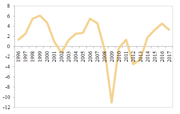
In this context, the investments cycle resumed at the end of 2013, with fixed investments accelerating over the past quarters (the highest paces since 2007), as can be noticed in figure 1.
Figure 1. The dynamics of the gross fixed capital formation in Euroland (%, YoY)
Source: Eurostat, Banca Transilvania
The relaunch of the fixed investments was also supported by the strong dynamics of the exports, given the global recovery and the increase of the international competitiveness of the region.
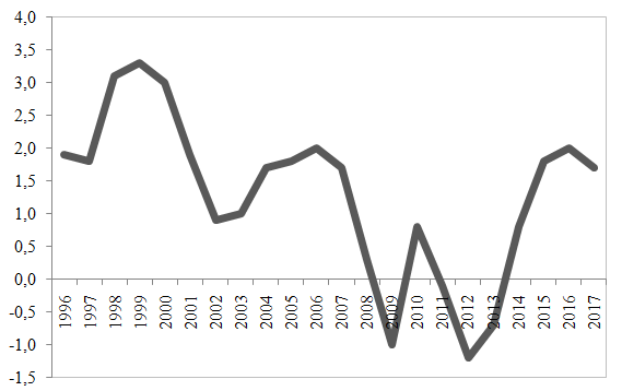
In this context, the labour markets climate presented an improvement trend over the past years (with the unemployment rate converging to the pre-crisis levels). This aspect corroborated with the relaunch of the credit markets fuelled the recovery of the private consumption in the Euroland (the main component of the GDP), as can be noticed from the following graph.
Figure 2. The evolution of the private consumption in the Euro Zone (%, YoY)
Source: Eurostat, Banca Transilvania
At the same time, the public consumption also increased starting 2013, as the manoeuvre room of the governments improved, given the fiscal consolidation, a process also supported by the record low level of the financing costs. The public consumption accelerated from 0.3% YoY in 2013 to 0.7% YoY in 2014, 1.3% YoY in 2015 and 1.8% YoY in 2016, according to the data published by Eurostat.
Last, but not least, the sustainable relaunch of the economy contributed to the improvement of the dynamics of the potential output over the past years.
On the other hand, the Euroland continues to face a low level of inflation (1.3% YoY in January 2018), below the target of the central bank (2% YoY). In this context, we point out that the monetary policy divergence (Federal Reserve vs. Euroland) seems not sustainable.
Furthermore, the global economic cycle has entered the maturity phase of the cycle, while in the region the manoeuvre space of the policy mix in the scenario of the incidence of adverse economic shocks is low.
3. METHODOLOGY
In order to assess the economic convergence in the Euroland we estimate the dynamics of the potential GDP and the output gap for the countries in the region by applying the Cobb-Douglas production function.
Afterwards, we compute the standard deviation for the cyclical and structural components of the GDP for the states members of the Euro Area.
As regards the Cobb-Douglas production function it is expressed in the following relation:
|
where Y, L, K, TFP and α represent the GDP, the labour factor, the capital stock, the total factor productivity and the output elasticity of labour.
By applying logarithms the relation (1.1) turns into:
|
where Yt, Lt, Kt and TFPt are the YoY paces for GDP, labour factor, capital stock and the total factor productivity.
In order to obtain the dynamics of the potential GDP we estimated the structural component (the trend) for the labour factor and for the total factor productivity, by applying the Hodrick-Prescott methodology.
The dynamics of the potential GDP can be expressed as in the following relation:
|
where Yt*, Lt* and TFPt* represent the trend component for the dynamics of the GDP, labour factor and total factor productivity.
The labour factor (L) was defined as:
|
As regards the capital stock we implemented the perpetuity method:
|
where Kt is the capital stock from year t, , d – the depreciation ratio and GFCFt – the gross fixed capital formation from year t.
In this paper we considered the capital stock for the member countries of the Euroland from 1995, as estimated in the paper of Derbyshire, et al. (2010) and an annual depreciation ratio of 5%.
As regards the GDP, the components of the labour factor and the gross fixed capital formation we utilised the Eurostat database (annual data, for the period 1996-2016).
In our study all the variables (as presented in relation (1.2) were divided by the population in each of the member states of Euroland.
The total factor productivity (the structural component) was estimated by applying the Hodrick-Prescot filter for the TFPt series, determined as:
|
We considered α = 0,65, as also utilised in the paper of D’Auria, et al. (2010).
As regards the Hodrick-Prescott filter, this can be expressed by the following relation:
|
(1.7) |
where Yt, Yt* şi ![]() represent the dynamics of GDP, of the potential GDP and the adjustment parameter („smoothness”): the lower the value of this indicator the dynamics of the GDP is closer to the potential pace.
represent the dynamics of GDP, of the potential GDP and the adjustment parameter („smoothness”): the lower the value of this indicator the dynamics of the GDP is closer to the potential pace.
In their paper Hodrick and Prescott (1997) considered a level of 100 for ![]() while working with annual data.
while working with annual data.
This filter is one of the most used methods by the macroeconomists in order to distinguish between the cyclical and structural components of the macroeconomic variables. However, this method also presents some shortcomings, including the „leakage effects” and the „compression effects”.
After estimating the cyclical and structural components of the GDP of the member countries in the Euroland we computed the dispersion (σ2) and the standard deviation (σ), according to the following relation:
|
where xi is the structural / cyclical component for GDP/capita in country i from Euro Zone, while ![]() is the structural / cyclical component of the Euroland GDP/capita (considered as YoY paces).
is the structural / cyclical component of the Euroland GDP/capita (considered as YoY paces).
We point out that the analysis of the structural component of the GDP/capita may reveal the structural reforms needed to the implemented by the countries in order to improve the economic convergence process.
On the other hand, the analysis of the cyclical component (the convergence of the cycles, in line with the Optimal Currency Area theory) allows us to identify the measures needed to be implemented for a better coordination of the macroeconomic policies within Euroland.
4. THE MAIN RESULTS
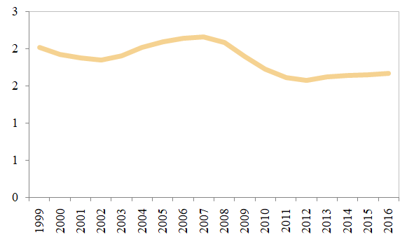
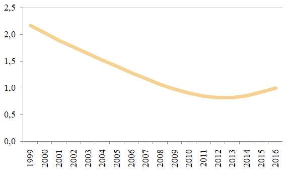
According to our results the standard deviation for the GDP/capita across the Euroland member countries consolidated around the record low levels over the past years, as can be noticed in the following graph.
Figure 3. The standard deviation for GDP/capita (Euroland member countries) (MA4)
Source: own estimates based on the methodology, using Eurostat, AMECO databases
This result expresses the fact that the real economic convergence within the Euroland consolidated over the past years, in the context of the post-crisis recovery, which was synchronized, under the influence of the New Economic Governance implemented after 2012.
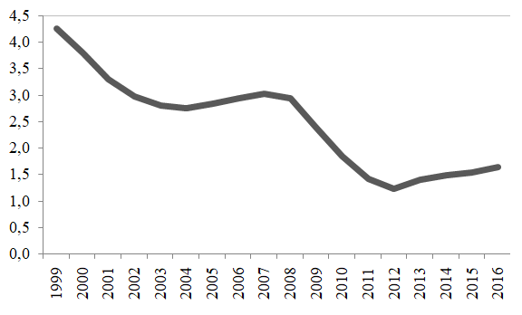
However, there can be noticed that the downward trend was recently interrupted, an evolution determined by the slowing down of the structural reforms, with impact for the dynamics of the capital stock and total factor productivity, as can be seen in the following figures.
Our results confirms the fact that despite the improvement of the macro-financial climate within the post-crisis cycle there remain important gaps among the member countries of the Euroland in terms of investments (including efficiency) and total factor productivity.
These differences are mainly structural and cannot be narrowed without significant investments (especially in high value added sectors) and structural reforms, needed to improve the contribution of the total factor productivity.
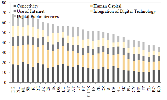
In this context, we mention the important differences in terms of Digitalisation (an important issue, given the Fourth Industrial Revolution), as reflected by Figure 6.
Figure 4. The standard deviation for capital stock/capita (Euroland member countries) (MA4)
Source: own estimates based on the methodology, using Eurostat, AMECO databases
Figure 5. The standard deviation for total factor productivity/capita (Euroland member countries) (MA4)
Source: own estimates based on the methodology, using Eurostat, AMECO databases
Figure 6. The Digital Economy in EU
Source: European Commission
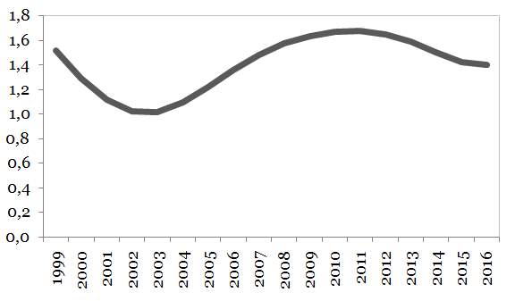
On the other hand, the convergence in terms of labour/capita continued to improve over the past quarters, in convergence towards the pre-crisis levels, as can be noticed in the following graph. This evolution was influenced by the recovery of the labour markets (given the post-crisis investment cycle) and by the implementation of several reforms after the incidence of the Great Recession, with impact for the mobility of active population (including the non-EU citizens).
Figure 7. The standard deviation for labour/capita (Euroland member countries) (MA4)
Source: own estimates based on the methodology, using Eurostat, AMECO databases
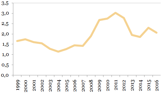
Last, but not least, our results also show the significant improvement of the cyclical convergence of the Euroland member countries over the past years, in convergence towards the pre-crisis levels, as can be noticed in the following figure.
Figure 8. The standard deviation for output gap (Euroland member countries) (MA4)
Source: own estimates based on the methodology, using Eurostat, AMECO databases
5. CONCLUSIONS
According to this analysis the economic convergence process of the Euro Zone member countries improved over the past years, an evolution determined by the implementation of the New Economic Governance (after the incidence of the Great Recession).
In this context, we point out that the unprecedented expansionary policy implemented by the European Central Bank contributed to the strengthening of the cyclical convergence.
On the other hand, we underline the fact that there persist structural differences across the member states of the Euroland, especially in terms of capital stock and total factor productivity.
Consequently, we consider that countries from the Euro Zone should continue the structural reforms (especially in a context of low (affordable) level of the financing costs) and should intensify the efforts in terms of implementing the Digital Revolution.
These reforms are important to consolidate the region and to better address the challenges during the next cyclical crisis.
BIBLIOGRAPHY
Banca Transilvania Research, https://www.bancatransilvania.ro/rapoarte-de-analiza/macroeconomie/
D’Auria, F., et al. 2010. The production function methodology for calculating potential growth rates and output gaps. European Commission Economic Papers, 420. Disponibil la http://ec.europa.eu/economy_finance/publications/economic_paper/2010/ecp420_en.htm
Derbyshire, J., Gardiner, B. and Waights, S., 2010. Estimating the capital stock for the NUTS2 regions of the EU-27, European Union Regional Policy, 1. Disponibil la http://ec.europa.eu/regional_policy/sources/docgener/work/2011_01_capital_stock.pdf
Dobrescu, E., 2006. Macromodels of the Romanian Market Economy. Bucharest: Economica.
Dobrescu, E., 2009. Estimating the Total Factor Productivity in Romanian Economy. Amfiteatru Economic, 26, pp. 512-521.
Eurostat. http://epp.eurostat.ec.europa.eu/portal/page/portal/eurostat/home/
Hodrick, R. and Prescott, E. C., 1997. Postwar U.S. Business Cycles: An Empirical Investigation. Journal of Money, Credit and Banking, 29 (1), pp. 1-16.
Document information
Published on 11/05/18
Accepted on 11/05/18
Submitted on 28/02/18
Licence: Other
