m (Cinmemj moved page Draft Samper 447947970 to Gonzalez et al 2011a) |
|||
| (16 intermediate revisions by the same user not shown) | |||
| Line 1: | Line 1: | ||
| − | |||
| − | |||
| − | |||
| − | |||
| − | |||
| − | |||
| − | |||
| − | |||
| − | |||
| − | |||
| − | |||
| − | |||
| − | |||
| − | |||
| − | |||
| − | |||
| − | |||
| − | |||
| − | |||
| − | |||
| − | |||
| − | |||
| − | |||
| − | |||
| − | |||
| − | |||
| − | |||
| − | |||
| − | |||
| − | |||
| − | |||
| − | |||
| − | |||
| − | |||
| − | |||
| − | |||
| − | |||
| − | |||
| − | |||
| − | |||
| − | |||
| − | |||
| − | |||
| − | |||
| − | |||
| − | |||
| − | |||
| − | |||
| − | |||
| − | |||
| − | |||
| − | |||
| − | |||
| − | |||
| − | |||
| − | |||
| − | |||
| − | |||
| − | |||
| − | |||
| − | |||
| − | |||
| − | |||
| − | |||
| − | |||
| − | |||
| − | |||
| − | |||
| − | |||
| − | |||
| − | |||
| − | |||
| − | |||
| − | |||
| − | |||
| − | |||
<span id='_Toc290547646'></span> | <span id='_Toc290547646'></span> | ||
| − | ==1. | + | ==1. Introduction== |
Gliding parachutes offer considerable scope for a large number of civil, humanitarian and military applications due to their ability to cover large horizontal distances from the drop point and their excellent controllability. A concept in the gliding-parachute category which has received attention since mid 60’s is the ram-air inflated fabric wing (also known as Jalbert parafoil or simply parafoil). Parafoils consist of a flexible fabric wing with rectangular planform and a streamlined cross-section which is opened at the leading edge to allow air to enter and inflate the wing to a specified shape. The payload is suspended on lines below the wing. Some of the earliest projects involving the usage of parafoil-based systems are discussed by Nikolaides and Knapp<sup>.1-7</sup> and comprehensive bibliography up to 1980 is provided by Lingard<sup>8</sup>. Moreover, some definitions that in the last quarter of the twentieth century have become a sort of standard and discussion on modern parafoil design are given by Poynter<sup>9</sup>. | Gliding parachutes offer considerable scope for a large number of civil, humanitarian and military applications due to their ability to cover large horizontal distances from the drop point and their excellent controllability. A concept in the gliding-parachute category which has received attention since mid 60’s is the ram-air inflated fabric wing (also known as Jalbert parafoil or simply parafoil). Parafoils consist of a flexible fabric wing with rectangular planform and a streamlined cross-section which is opened at the leading edge to allow air to enter and inflate the wing to a specified shape. The payload is suspended on lines below the wing. Some of the earliest projects involving the usage of parafoil-based systems are discussed by Nikolaides and Knapp<sup>.1-7</sup> and comprehensive bibliography up to 1980 is provided by Lingard<sup>8</sup>. Moreover, some definitions that in the last quarter of the twentieth century have become a sort of standard and discussion on modern parafoil design are given by Poynter<sup>9</sup>. | ||
| Line 109: | Line 33: | ||
<div class="center" style="width: auto; margin-left: auto; margin-right: auto;"> | <div class="center" style="width: auto; margin-left: auto; margin-right: auto;"> | ||
| − | <span style="text-align: center; font-size: 75%;">Figure 1. Parafoil and payload schematic.</span></div> | + | <span style="text-align: center; font-size: 75%;">'''Figure 1'''. Parafoil and payload schematic.</span></div> |
| + | |||
The kinematic of the parafoil-payload system can be defined by | The kinematic of the parafoil-payload system can be defined by | ||
| − | + | {| style="width: 100%; text-align: left;" | |
| − | + | |- | |
| + | | style="text-align: center;" | [[Image:draft_Samper_447947970-image21.png|96px]] | ||
| + | | style="text-align: right;vertical-align: center;width: 5px;text-align: right;white-space: nowrap;"|(1) | ||
| + | |} | ||
| + | |||
| + | |||
| + | {| style="width: 100%; text-align: left;" | ||
| + | |- | ||
| + | | style="text-align: center;" | [[Image:draft_Samper_447947970-image22.png|252px]] | ||
| + | | style="text-align: right;vertical-align: center;width: 5px;text-align: right;white-space: nowrap;"|(2) | ||
| + | |} | ||
| − | |||
| − | |||
where T<sub>IB</sub> is the transformation matrix from an inertial reference frame to the body reference frame | where T<sub>IB</sub> is the transformation matrix from an inertial reference frame to the body reference frame | ||
| − | + | ||
| − | [[Image:draft_Samper_447947970-image23.png|480px]] () | + | {| style="width: 100%; text-align: left;" |
| + | |- | ||
| + | | style="text-align: center;" | [[Image:draft_Samper_447947970-image23.png|480px]] | ||
| + | | style="text-align: right;vertical-align: center;width: 5px;text-align: right;white-space: nowrap;"|(3) | ||
| + | |} | ||
| + | |||
The equations of motion of the parachute-payload system can be obtained by summing up forces and moment contributions about the system centre of gravity (CG). Thus, | The equations of motion of the parachute-payload system can be obtained by summing up forces and moment contributions about the system centre of gravity (CG). Thus, | ||
| − | + | {| style="width: 100%; text-align: left;" | |
| − | + | |- | |
| + | | style="text-align: center;" | | ||
| + | [[File:Draft_Samper_447947970_4683_ec4.png|240px]] | ||
| + | | style="text-align: right;vertical-align: center;width: 5px;text-align: right;white-space: nowrap;"|(4) | ||
| + | |} | ||
| + | |||
| + | |||
| + | {| style="width: 100%; text-align: left;" | ||
| + | |- | ||
| + | | style="text-align: center;" | | ||
| + | [[File:Draft_Samper_447947970_4859_ec5.png|498px]] | ||
| + | | style="text-align: right;vertical-align: center;width: 5px;text-align: right;white-space: nowrap;"|(5) | ||
| + | |} | ||
| − | |||
| − | |||
The following convention is used for the vector cross product of two vectors''' r''' = {r<sub>x</sub> r<sub>y</sub> r<sub>z</sub>}<sup>T</sup> and '''F''' = {F<sub>x</sub> F<sub>y</sub> F<sub>z</sub>}<sup>T</sup> both expressed in the aerodynamic reference frame | The following convention is used for the vector cross product of two vectors''' r''' = {r<sub>x</sub> r<sub>y</sub> r<sub>z</sub>}<sup>T</sup> and '''F''' = {F<sub>x</sub> F<sub>y</sub> F<sub>z</sub>}<sup>T</sup> both expressed in the aerodynamic reference frame | ||
| − | + | {| style="width: 100%; text-align: left;" | |
| − | [[Image:draft_Samper_447947970-image26.png|204px]] () | + | |- |
| + | | style="text-align: center;" | [[Image:draft_Samper_447947970-image26.png|204px]] | ||
| + | | style="text-align: right;vertical-align: center;width: 5px;text-align: right;white-space: nowrap;"|(6) | ||
| + | |} | ||
| + | |||
The forces appearing in Eq. (4) are the weight ('''F'''<sub>W</sub>), the canopy aerodynamic load ('''F'''<sub>A</sub>), the payload aerodynamic load ('''F'''<sub>S</sub>) and the apparent mass forces ('''F'''<sub>AM</sub>). These contributions are developed in the following equations. | The forces appearing in Eq. (4) are the weight ('''F'''<sub>W</sub>), the canopy aerodynamic load ('''F'''<sub>A</sub>), the payload aerodynamic load ('''F'''<sub>S</sub>) and the apparent mass forces ('''F'''<sub>AM</sub>). These contributions are developed in the following equations. | ||
| Line 141: | Line 93: | ||
Starting with the weight contribution, we can define | Starting with the weight contribution, we can define | ||
| − | + | {| style="width: 100%; text-align: left;" | |
| − | [[Image:draft_Samper_447947970-image27.png|132px]] () | + | |- |
| + | | style="text-align: center;" | [[Image:draft_Samper_447947970-image27.png|132px]] | ||
| + | | style="text-align: right;vertical-align: center;width: 5px;text-align: right;white-space: nowrap;"|(7) | ||
| + | |} | ||
| + | |||
Then, before defining aerodynamic forces, the aerodynamic velocities and angles are written in terms of the wind components and the canopy relative angle of incidence. Thus, | Then, before defining aerodynamic forces, the aerodynamic velocities and angles are written in terms of the wind components and the canopy relative angle of incidence. Thus, | ||
| − | + | {| style="width: 100%; text-align: left;" | |
| − | [[Image:draft_Samper_447947970-image28.png|390px]] () | + | |- |
| + | | style="text-align: center;" | [[Image:draft_Samper_447947970-image28.png|390px]] | ||
| + | | style="text-align: right;vertical-align: center;width: 5px;text-align: right;white-space: nowrap;"|(8) | ||
| + | |} | ||
| − | |||
| − | |||
| − | + | {| style="width: 100%; text-align: left;" | |
| − | [[Image:draft_Samper_447947970- | + | |- |
| + | | style="text-align: center;" | [[Image:draft_Samper_447947970-image29.png|78px]] | ||
| + | | style="text-align: right;vertical-align: center;width: 5px;text-align: right;white-space: nowrap;"|(9) | ||
| + | |} | ||
| − | + | ||
| − | [[Image:draft_Samper_447947970-image31.png|126px]] () | + | {| style="width: 100%; text-align: left;" |
| + | |- | ||
| + | | style="text-align: center;" | [[Image:draft_Samper_447947970-image30.png|90px]] | ||
| + | | style="text-align: right;vertical-align: center;width: 5px;text-align: right;white-space: nowrap;"|(10) | ||
| + | |} | ||
| + | |||
| + | |||
| + | {| style="width: 100%; text-align: left;" | ||
| + | |- | ||
| + | | style="text-align: center;" | [[Image:draft_Samper_447947970-image31.png|126px]] | ||
| + | | style="text-align: right;vertical-align: center;width: 5px;text-align: right;white-space: nowrap;"|(11) | ||
| + | |} | ||
where the transformation from body to canopy reference frames can be expressed by | where the transformation from body to canopy reference frames can be expressed by | ||
| − | + | {| style="width: 100%; text-align: left;" | |
| − | + | |- | |
| + | | style="text-align: center;" | [[Image:draft_Samper_447947970-image32.png|162px]] | ||
| + | | style="text-align: right;vertical-align: center;width: 5px;text-align: right;white-space: nowrap;"|(12) | ||
| + | |} | ||
| + | |||
The aerodynamic force is defined in terms of aerodynamic derivatives (these are considered known data). Thus, | The aerodynamic force is defined in terms of aerodynamic derivatives (these are considered known data). Thus, | ||
| − | + | {| style="width: 100%; text-align: left;" | |
| − | + | |- | |
| + | | style="text-align: center;" |[[Image:draft_Samper_447947970-image33.png|312px]] | ||
| + | | style="text-align: right;vertical-align: center;width: 5px;text-align: right;white-space: nowrap;"|(13) | ||
| + | |} | ||
| + | |||
with '''T'''<sub>AB</sub> being the transformation from the aerodynamic to canopy reference frame | with '''T'''<sub>AB</sub> being the transformation from the aerodynamic to canopy reference frame | ||
| − | + | {| style="width: 100%; text-align: left;" | |
| − | + | |- | |
| + | | style="text-align: center;" | [[Image:draft_Samper_447947970-image34.png|342px]] | ||
| + | | style="text-align: right;vertical-align: center;width: 5px;text-align: right;white-space: nowrap;"|(14) | ||
| + | |} | ||
| + | |||
The only force taken into account for the payload is the drag. This is expressed in terms of its own local velocity (in the body reference frame) by | The only force taken into account for the payload is the drag. This is expressed in terms of its own local velocity (in the body reference frame) by | ||
| − | + | {| style="width: 100%; text-align: left;" | |
| − | + | |- | |
| + | | style="text-align: center;" |[[Image:draft_Samper_447947970-image35.png|156px]] | ||
| + | | style="text-align: right;vertical-align: center;width: 5px;text-align: right;white-space: nowrap;"|(15) | ||
| + | |} | ||
| + | |||
Besides the forces contribution to the total system moment, there are two additional terms in Eq. (5) that correspond to aerodynamic and apparent mass moments. Similar to the aerodynamic forces, the aerodynamic moment is defined in terms of derivatives | Besides the forces contribution to the total system moment, there are two additional terms in Eq. (5) that correspond to aerodynamic and apparent mass moments. Similar to the aerodynamic forces, the aerodynamic moment is defined in terms of derivatives | ||
| − | + | {| style="width: 100%; text-align: left;" | |
| − | + | |- | |
| + | | style="text-align: center;" |[[Image:draft_Samper_447947970-image36.png|462px]] | ||
| + | | style="text-align: right;vertical-align: center;width: 5px;text-align: right;white-space: nowrap;"|(16) | ||
| + | |} | ||
| + | |||
As the parafoil moves through the air, it displaces and accelerates the fluid surrounding it. The apparent mass effect is defined as the reaction of the fluid surrounding the parafoil. In high mass-to-volume ratio bodies like airplanes this reaction is negligible, but in very light vehicles like parafoils it plays an important role and can significantly affect their behaviour. A common practice is to add this effect as additional mass and inertia terms named “apparent mass” and “apparent inertia” which can be derived from the total kinetic energy of the fluid set in motion along with the parafoil. According to Lamb<sup>27</sup>, the kinetic energy can be expressed for a typical parachute canopy having two planes of symmetry, x-z and y-z, by | As the parafoil moves through the air, it displaces and accelerates the fluid surrounding it. The apparent mass effect is defined as the reaction of the fluid surrounding the parafoil. In high mass-to-volume ratio bodies like airplanes this reaction is negligible, but in very light vehicles like parafoils it plays an important role and can significantly affect their behaviour. A common practice is to add this effect as additional mass and inertia terms named “apparent mass” and “apparent inertia” which can be derived from the total kinetic energy of the fluid set in motion along with the parafoil. According to Lamb<sup>27</sup>, the kinetic energy can be expressed for a typical parachute canopy having two planes of symmetry, x-z and y-z, by | ||
| − | + | {| style="width: 100%; text-align: left;" | |
| − | + | |- | |
| + | | style="text-align: center;" | [[Image:draft_Samper_447947970-image37.png|366px]] | ||
| + | | style="text-align: right;vertical-align: center;width: 5px;text-align: right;white-space: nowrap;"|(17) | ||
| + | |} | ||
| + | |||
where the seven constants are defined in terms of parachute geometric parameters. In addition, if we neglect the spanwise camber effect, the constant H can be considered to be zero (this is the approach adopted here). Therefore, using the formulae given by Lissaman and Brown<sup>24</sup>, the apparent mass terms A, B, C, P, Q and R can be computed as follows | where the seven constants are defined in terms of parachute geometric parameters. In addition, if we neglect the spanwise camber effect, the constant H can be considered to be zero (this is the approach adopted here). Therefore, using the formulae given by Lissaman and Brown<sup>24</sup>, the apparent mass terms A, B, C, P, Q and R can be computed as follows | ||
| − | + | {| style="width: 100%; text-align: left;" | |
| − | [[Image:draft_Samper_447947970-image38.png|174px]] () | + | |- |
| + | | style="text-align: center;" | [[Image:draft_Samper_447947970-image38.png|174px]] | ||
| + | | style="text-align: right;vertical-align: center;width: 5px;text-align: right;white-space: nowrap;"|(18) | ||
| + | |} | ||
| − | |||
| − | |||
| − | + | {| style="width: 100%; text-align: left;" | |
| − | + | |- | |
| + | | style="text-align: center;" | [[Image:draft_Samper_447947970-image39.png|216px]] | ||
| + | | style="text-align: right;vertical-align: center;width: 5px;text-align: right;white-space: nowrap;"|(19) | ||
| + | |} | ||
| − | |||
| − | |||
| − | + | {| style="width: 100%; text-align: left;" | |
| − | [[Image:draft_Samper_447947970-image42.png|372px]] () | + | |- |
| + | | style="text-align: center;" | [[Image:draft_Samper_447947970-image40.png|294px]] | ||
| + | | style="text-align: right;vertical-align: center;width: 5px;text-align: right;white-space: nowrap;"|(20) | ||
| + | |} | ||
| + | |||
| + | |||
| + | {| style="width: 100%; text-align: left;" | ||
| + | |- | ||
| + | | style="text-align: center;" | [[Image:draft_Samper_447947970-image41.png|150px]] | ||
| + | | style="text-align: right;vertical-align: center;width: 5px;text-align: right;white-space: nowrap;"|(21) | ||
| + | |} | ||
| + | |||
| + | |||
| + | {| style="width: 100%; text-align: left;" | ||
| + | |- | ||
| + | | style="text-align: center;" |[[Image:draft_Samper_447947970-image42.png|372px]] | ||
| + | | style="text-align: right;vertical-align: center;width: 5px;text-align: right;white-space: nowrap;"|(22) | ||
| + | |} | ||
| + | |||
| + | |||
| + | {| style="width: 100%; text-align: left;" | ||
| + | |- | ||
| + | | style="text-align: center;" | [[Image:draft_Samper_447947970-image43.png|162px]] | ||
| + | | style="text-align: right;vertical-align: center;width: 5px;text-align: right;white-space: nowrap;"|(23) | ||
| + | |} | ||
| − | |||
| − | |||
Then, forces and moments due to apparent mass and inertia can be obtained by relating the momentum of the fluid surrounding the parafoil to its kinetic energy. Following Lissman and Brown, | Then, forces and moments due to apparent mass and inertia can be obtained by relating the momentum of the fluid surrounding the parafoil to its kinetic energy. Following Lissman and Brown, | ||
| − | + | {| style="width: 100%; text-align: left;" | |
| − | + | |- | |
| + | | style="text-align: center;" | [[Image:draft_Samper_447947970-image44.png|264px]] | ||
| + | | style="text-align: right;vertical-align: center;width: 5px;text-align: right;white-space: nowrap;"|(24) | ||
| + | |} | ||
| − | |||
| − | |||
| − | + | {| style="width: 100%; text-align: left;" | |
| − | + | |- | |
| + | | style="text-align: center;" |[[Image:draft_Samper_447947970-image45.png|234px]] | ||
| + | | style="text-align: right;vertical-align: center;width: 5px;text-align: right;white-space: nowrap;"|(25) | ||
| + | |} | ||
| − | + | ||
| − | + | {| style="width: 100%; text-align: left;" | |
| + | |- | ||
| + | | style="text-align: center;" |[[Image:draft_Samper_447947970-image46.png|120px]] | ||
| + | | style="text-align: right;vertical-align: center;width: 5px;text-align: right;white-space: nowrap;"|(26) | ||
| + | |} | ||
| + | |||
| + | |||
| + | {| style="width: 100%; text-align: left;" | ||
| + | |- | ||
| + | | style="text-align: center;" |[[Image:draft_Samper_447947970-image47.png|120px]] | ||
| + | | style="text-align: right;vertical-align: center;width: 5px;text-align: right;white-space: nowrap;"|(27) | ||
| + | |} | ||
Finally, the set of dynamic equations of motion is obtained by replacing all the previous forces and moments into Eqs. (4) and (5). Thus, | Finally, the set of dynamic equations of motion is obtained by replacing all the previous forces and moments into Eqs. (4) and (5). Thus, | ||
| − | + | {| style="width: 100%; text-align: left;" | |
| − | + | |- | |
| + | | style="text-align: center;" |[[Image:draft_Samper_447947970-image48.png|378px]] | ||
| + | | style="text-align: right;vertical-align: center;width: 5px;text-align: right;white-space: nowrap;"|(28) | ||
| + | |} | ||
| − | |||
| − | |||
| − | + | {| style="width: 100%; text-align: left;" | |
| − | + | |- | |
| + | | style="text-align: center;" | [[Image:draft_Samper_447947970-image49.png|486px]] | ||
| + | | style="text-align: right;vertical-align: center;width: 5px;text-align: right;white-space: nowrap;"|(29) | ||
| + | |} | ||
| + | |||
| + | |||
| + | {| style="width: 100%; text-align: left;" | ||
| + | |- | ||
| + | | style="text-align: center;" |[[Image:draft_Samper_447947970-image50.png|492px]] | ||
| + | | style="text-align: right;vertical-align: center;width: 5px;white-space: nowrap;"|(30) | ||
| + | |} | ||
| + | |||
where the following notation applies | where the following notation applies | ||
| − | + | {| style="width: 100%; text-align: left;" | |
| − | + | |- | |
| + | | style="text-align: center;" |[[Image:draft_Samper_447947970-image51.png|138px]] | ||
| + | | style="text-align: right;vertical-align: center;width: 5px;white-space: nowrap;"|(31) | ||
| + | |} | ||
| + | |||
In the matrix in Eq. (29) it is possible to observe that apparent mass effects couple linear and rotational dynamics, which would be decoupled otherwise (in models where apparent mass coefficients are constant). | In the matrix in Eq. (29) it is possible to observe that apparent mass effects couple linear and rotational dynamics, which would be decoupled otherwise (in models where apparent mass coefficients are constant). | ||
| Line 256: | Line 306: | ||
<div class="center" style="width: auto; margin-left: auto; margin-right: auto;"> | <div class="center" style="width: auto; margin-left: auto; margin-right: auto;"> | ||
| − | <span style="text-align: center; font-size: 75%;">Figure 2. Lateral control strategy.</span></div> | + | <span style="text-align: center; font-size: 75%;">'''Figure 2'''. Lateral control strategy.</span></div> |
| + | |||
The control strategy proceeds as follows. For a given parachute track position <math display="inline">\left(X_{track},Y_{track}\right)</math> , measured from '''W''' ''<sub>p2</sub>'', the vehicle ground velocity vector <math display="inline">V_{ground}</math> is pointed in the direction of a line intercepting the track at point ''C''. The interception point ''C'' is determined by considering that the distance on the track line from this point to ''W<sub>p2</sub>'' is, at any instant time, equal to <math display="inline">(1-k)\mbox{ }X_{track}</math> , being ''k'' a design parameter. From the geometry of the similar triangles ''OAB'' and ''OCD'', the parachute position and velocity is established according to | The control strategy proceeds as follows. For a given parachute track position <math display="inline">\left(X_{track},Y_{track}\right)</math> , measured from '''W''' ''<sub>p2</sub>'', the vehicle ground velocity vector <math display="inline">V_{ground}</math> is pointed in the direction of a line intercepting the track at point ''C''. The interception point ''C'' is determined by considering that the distance on the track line from this point to ''W<sub>p2</sub>'' is, at any instant time, equal to <math display="inline">(1-k)\mbox{ }X_{track}</math> , being ''k'' a design parameter. From the geometry of the similar triangles ''OAB'' and ''OCD'', the parachute position and velocity is established according to | ||
| − | + | {| style="width: 100%; text-align: left;" | |
| − | <math>\frac{{\dot{X}}_{track}}{k\cdot X_{track}}=\frac{{\dot{Y}}_{track}}{Y_{track}}</math> () | + | |- |
| + | | style="text-align: center;" | <math>\frac{{\dot{X}}_{track}}{k\cdot X_{track}}=\frac{{\dot{Y}}_{track}}{Y_{track}}</math> | ||
| + | | style="text-align: right;vertical-align: center;width: 5px;text-align: right;white-space: nowrap;"|(32) | ||
| + | |} | ||
Accordingly, an error ''E'' is defined by | Accordingly, an error ''E'' is defined by | ||
| − | |||
| − | |||
| − | + | {| style="width: 100%; text-align: left;" | |
| + | |- | ||
| + | | style="text-align: center;" | <math>E=k\cdot X_{track}{\dot{Y}}_{track}-Y_{track}{\dot{X}}_{track}=0</math> | ||
| + | | style="text-align: right;vertical-align: center;width: 5px;text-align: right;white-space: nowrap;"|(33) | ||
| + | |} | ||
| − | |||
| − | |||
| − | |||
| − | + | If Eq. (33) is not satisfied (meaning that there is a heading error), the magnitude and sign of error ''E'' is used to define a parachute brake command. This is done in two steps: first a “desired yaw-rate” is defined and then parachute brakes are pulled in order to obtain it. The “desired yaw-rate” is defined as follows, | |
| − | + | ||
| − | where [[Image:draft_Samper_447947970- | + | {| style="width: 100%; text-align: left;" |
| + | |- | ||
| + | | style="text-align: center;" | <math>r_{CMD}=K_RE=K_R\left(k\cdot X_{track}{\dot{Y}}_{track}- Y_{track}{\dot{X}}_{track}\right)</math> | ||
| + | | style="text-align: right;vertical-align: center;width: 5px;text-align: right;white-space: nowrap;"|(34) | ||
| + | |} | ||
| + | |||
| + | |||
| + | where the proportional gain <math display="inline">K_{r}</math> should be determined iteratively in order to achieve good tracking without overshoots. Moreover, the yaw-rate is limited to <math display="inline">R_{\max}=\pm 0.2</math> rad/s with the aim of avoiding numerical misbehaviours. To command the parachute, brakes are actuated by comparison of the “desired yaw-rate” with the actual yaw-rate. If there is a difference, a brake input is generated left or right, depending on the sign resulting from the comparison. This process is summarized in the following expression, | ||
| + | |||
| + | {| style="width: 100%; text-align: left;" | ||
| + | |- | ||
| + | | style="text-align: center;" | [[Image:draft_Samper_447947970-image61.png|150px]] | ||
| + | | style="text-align: right;vertical-align: center;width: 5px;text-align: right;white-space: nowrap;"|(35) | ||
| + | |} | ||
| + | |||
| + | |||
| + | where <math display="inline">K_{brake}</math> is a constant taking into account the kinematics of the parachute brake line. | ||
<span id='_Toc280563188'></span><span id='_Toc290547651'></span> | <span id='_Toc280563188'></span><span id='_Toc290547651'></span> | ||
| Line 286: | Line 354: | ||
Parafoil altitude control deals with potential energy management. The altitude control strategy adopted in this work divides the parafoil flight in three parts: an initial straight down gliding phase followed by a spiral descent phase and a final straight down approach towards the target. The first phase begins immediately after the parachute is deployed and extends until the target distance is reduced by a specified percentage. During this phase the parafoil uses only lateral control to navigate to the target and the travelled distance is recorded in order to evaluate an average parachute glide slope. At the beginning of the second phase, the control system computes an “ideal” flight altitude (''h<sub>ideal</sub>'') according to | Parafoil altitude control deals with potential energy management. The altitude control strategy adopted in this work divides the parafoil flight in three parts: an initial straight down gliding phase followed by a spiral descent phase and a final straight down approach towards the target. The first phase begins immediately after the parachute is deployed and extends until the target distance is reduced by a specified percentage. During this phase the parafoil uses only lateral control to navigate to the target and the travelled distance is recorded in order to evaluate an average parachute glide slope. At the beginning of the second phase, the control system computes an “ideal” flight altitude (''h<sub>ideal</sub>'') according to | ||
| − | + | {| style="width: 100%; text-align: left;" | |
| − | + | |- | |
| + | | style="text-align: center;" | [[Image:draft_Samper_447947970-image63.png|102px]] | ||
| + | | style="text-align: right;vertical-align: center;width: 5px;text-align: right;white-space: nowrap;"|(36) | ||
| + | |} | ||
where D<sub>target</sub> is the remaining distance to target and GS<sub>Phase_1</sub> is the average glideslope measured at the initial phase. If the real parachute altitude'' h<sub>real</sub>'' is greater than ''h<sub>ideal</sub>'', a spiral descent is initiated by a specified constant brake input which holds until ''h<sub>real</sub>'' < ''h<sub>ideal</sub>''. Otherwise, the descent is omitted because the parachute altitude could be insufficient to reach the target. The third flight phase begins when ''h<sub>real</sub>'' ≤ ''h<sub>ideal</sub>'' and involves the final approach. During this stage both lateral and glideslope controls are applied. The latter is implemented through a variable incidence angle which is determined by the following proportional control | where D<sub>target</sub> is the remaining distance to target and GS<sub>Phase_1</sub> is the average glideslope measured at the initial phase. If the real parachute altitude'' h<sub>real</sub>'' is greater than ''h<sub>ideal</sub>'', a spiral descent is initiated by a specified constant brake input which holds until ''h<sub>real</sub>'' < ''h<sub>ideal</sub>''. Otherwise, the descent is omitted because the parachute altitude could be insufficient to reach the target. The third flight phase begins when ''h<sub>real</sub>'' ≤ ''h<sub>ideal</sub>'' and involves the final approach. During this stage both lateral and glideslope controls are applied. The latter is implemented through a variable incidence angle which is determined by the following proportional control | ||
| − | + | {| style="width: 100%; text-align: left;" | |
| − | + | |- | |
| + | | style="text-align: center;" | [[Image:draft_Samper_447947970-image64.png|150px]] | ||
| + | | style="text-align: right;vertical-align: center;width: 5px;text-align: right;white-space: nowrap;"|(37) | ||
| + | |} | ||
| + | |||
where ''k<sub>p</sub>'' is the proportional gain. The incidence angle is increased (to the negative side) if the parafoil is higher than ''h<sub>ideal</sub>'' and decreased in the opposite case. This allows achieving a very fine adjustment of the glide slope as the parachute approaches to the target. | where ''k<sub>p</sub>'' is the proportional gain. The incidence angle is increased (to the negative side) if the parafoil is higher than ''h<sub>ideal</sub>'' and decreased in the opposite case. This allows achieving a very fine adjustment of the glide slope as the parachute approaches to the target. | ||
| Line 312: | Line 387: | ||
<div class="center" style="width: auto; margin-left: auto; margin-right: auto;"> | <div class="center" style="width: auto; margin-left: auto; margin-right: auto;"> | ||
| − | <span style="text-align: center; font-size: 75%;">Figure 3: Snowflake parafoil-payload system photo, geometry schematics and payload.</span></div> | + | <span style="text-align: center; font-size: 75%;">'''Figure 3''': Snowflake parafoil-payload system photo, geometry schematics and payload.</span></div> |
| + | |||
<div class="center" style="width: auto; margin-left: auto; margin-right: auto;"> | <div class="center" style="width: auto; margin-left: auto; margin-right: auto;"> | ||
| Line 318: | Line 394: | ||
<div class="center" style="width: auto; margin-left: auto; margin-right: auto;"> | <div class="center" style="width: auto; margin-left: auto; margin-right: auto;"> | ||
| − | <span style="text-align: center; font-size: 75%;">Table 1: Main characteristics of the Snowflake parachute-payload system.</span></div> | + | <span style="text-align: center; font-size: 75%;">'''Table 1''': Main characteristics of the Snowflake parachute-payload system.</span></div> |
| + | |||
| − | |||
<span id="fn-1"></span>([[#fnc-1|<sup>1</sup>]]) <span style="text-align: center; font-size: 75%;">It must be noticed that the data was provided by Prof. Slegers from the University of Alabama in a personal communication to the authors</span> | <span id="fn-1"></span>([[#fnc-1|<sup>1</sup>]]) <span style="text-align: center; font-size: 75%;">It must be noticed that the data was provided by Prof. Slegers from the University of Alabama in a personal communication to the authors</span> | ||
| Line 339: | Line 415: | ||
<div class="center" style="width: auto; margin-left: auto; margin-right: auto;"> | <div class="center" style="width: auto; margin-left: auto; margin-right: auto;"> | ||
| − | <span style="text-align: center; font-size: 75%;">Figure 4: Trajectory plots, flat view (left) and 3D view (right).</span></div> | + | <span style="text-align: center; font-size: 75%;">'''Figure 4''': Trajectory plots, flat view (left) and 3D view (right).</span></div> |
| + | |||
Next, the performance of the control algorithm is assessed by guiding the parachute-payload system through a flight path defined by waypoints '''W''' ''<sub>p1</sub>'' and '''W''' ''<sub>p2</sub>''. Figure 5 shows three flight paths computed for different values of design parameter ''k'' and heading angles. | Next, the performance of the control algorithm is assessed by guiding the parachute-payload system through a flight path defined by waypoints '''W''' ''<sub>p1</sub>'' and '''W''' ''<sub>p2</sub>''. Figure 5 shows three flight paths computed for different values of design parameter ''k'' and heading angles. | ||
| − | [[ | + | [[File:Draft_Samper_447947970_9658_Fig5.png|600px]] |
| + | |||
| + | <span style="text-align: center; font-size: 75%;">'''Figure 5'''. Left: influence of the design parameter k on the guided trajectory for a South release heading (180º). Right: automatic control response to different release heading angles (k = 0.8).</span> | ||
| − | |||
Figure 5 (left) shows that the trajectory is noticeably affected by the design parameter ''k''; in the present example smaller values of ''k'' lead to a faster track interception but with a considerable overshoot. Therefore, this parameter should be adjusted depending on the mission requirements As regards initial heading, Figure 5 (right) demonstrates that it is successfully managed by the control system even under the most adverse release conditions. | Figure 5 (left) shows that the trajectory is noticeably affected by the design parameter ''k''; in the present example smaller values of ''k'' lead to a faster track interception but with a considerable overshoot. Therefore, this parameter should be adjusted depending on the mission requirements As regards initial heading, Figure 5 (right) demonstrates that it is successfully managed by the control system even under the most adverse release conditions. | ||
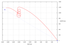
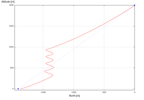
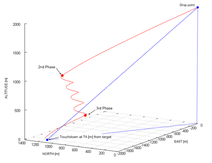
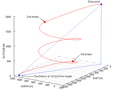
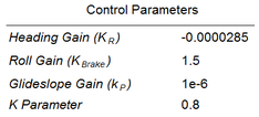
The second test applies full lateral and altitude control to a typical payload drop. The system is deployed at 2000 meters of altitude, 2200 meters away from the target, with wind coming from the south at 3 meters per second. Initially, the system navigates directly to the target regardless of the excess of altitude (Phase 1). When the horizontal distance to the target is reduced by 75% and spiral descent is performed until reaching ''h<sub>ideal</sub>'' (Phase 2). At this point, navigation to the target is re-engaged and glideslope control is activated (incidence angle variation, Phase 3). The computed trajectory is depicted in Figures 6 and 7. It should be noticed that although the parafoil touchdown took place at an acceptable distance from the target (74 meters), the precision could be further improved by fine tuning of the control gains. The gain parameters used in this simulation are presented in Table 2. | The second test applies full lateral and altitude control to a typical payload drop. The system is deployed at 2000 meters of altitude, 2200 meters away from the target, with wind coming from the south at 3 meters per second. Initially, the system navigates directly to the target regardless of the excess of altitude (Phase 1). When the horizontal distance to the target is reduced by 75% and spiral descent is performed until reaching ''h<sub>ideal</sub>'' (Phase 2). At this point, navigation to the target is re-engaged and glideslope control is activated (incidence angle variation, Phase 3). The computed trajectory is depicted in Figures 6 and 7. It should be noticed that although the parafoil touchdown took place at an acceptable distance from the target (74 meters), the precision could be further improved by fine tuning of the control gains. The gain parameters used in this simulation are presented in Table 2. | ||
| + | |||
<div class="center" style="width: auto; margin-left: auto; margin-right: auto;"> | <div class="center" style="width: auto; margin-left: auto; margin-right: auto;"> | ||
| Line 362: | Line 441: | ||
<div class="center" style="width: auto; margin-left: auto; margin-right: auto;"> | <div class="center" style="width: auto; margin-left: auto; margin-right: auto;"> | ||
| − | <span style="text-align: center; font-size: 75%;">Figure 6: Trajectory plots, flat view (left) and lateral view (right).</span></div> | + | <span style="text-align: center; font-size: 75%;">'''Figure 6''': Trajectory plots, flat view (left) and lateral view (right).</span></div> |
| + | |||
<div class="center" style="width: auto; margin-left: auto; margin-right: auto;"> | <div class="center" style="width: auto; margin-left: auto; margin-right: auto;"> | ||
| Line 368: | Line 448: | ||
<div class="center" style="width: auto; margin-left: auto; margin-right: auto;"> | <div class="center" style="width: auto; margin-left: auto; margin-right: auto;"> | ||
| − | <span style="text-align: center; font-size: 75%;">Table 2: Snowflake parachute-payload system control parameters</span></div> | + | <span style="text-align: center; font-size: 75%;">'''Table 2''': Snowflake parachute-payload system control parameters</span></div> |
| + | |||
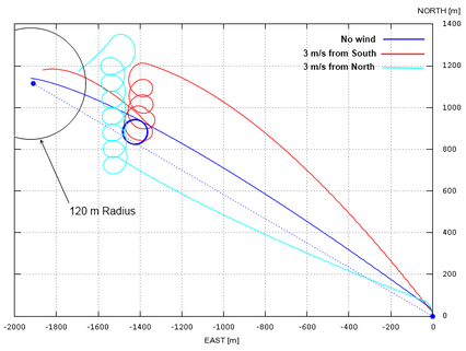
Finally, a similar test case is solved but this time considering wind effects. The simulation results are shown in Figure 8, where it can be observed that the control system has a very good performance in the no-wind condition but deteriorates with wing, a situation in which a strong dependance on its intensity and direction is identified. This behavior can be enhanced by taking into account wind conditions and relative position of the parafoil with respect to the target when the switch from flight phase 2 to phase 3 is computed. These strategies are currently a topic of investigation of many research groups, ''cf.'' Yakimenko<sup>29</sup> for an overview. | Finally, a similar test case is solved but this time considering wind effects. The simulation results are shown in Figure 8, where it can be observed that the control system has a very good performance in the no-wind condition but deteriorates with wing, a situation in which a strong dependance on its intensity and direction is identified. This behavior can be enhanced by taking into account wind conditions and relative position of the parafoil with respect to the target when the switch from flight phase 2 to phase 3 is computed. These strategies are currently a topic of investigation of many research groups, ''cf.'' Yakimenko<sup>29</sup> for an overview. | ||
| + | |||
<div class="center" style="width: auto; margin-left: auto; margin-right: auto;"> | <div class="center" style="width: auto; margin-left: auto; margin-right: auto;"> | ||
| Line 376: | Line 458: | ||
<div class="center" style="width: auto; margin-left: auto; margin-right: auto;"> | <div class="center" style="width: auto; margin-left: auto; margin-right: auto;"> | ||
| − | <span style="text-align: center; font-size: 75%;">Figure 7: 3D trajectory plot.</span></div> | + | <span style="text-align: center; font-size: 75%;">'''Figure 7''': 3D trajectory plot.</span></div> |
| + | |||
<div class="center" style="width: auto; margin-left: auto; margin-right: auto;"> | <div class="center" style="width: auto; margin-left: auto; margin-right: auto;"> | ||
| Line 382: | Line 465: | ||
<div class="center" style="width: auto; margin-left: auto; margin-right: auto;"> | <div class="center" style="width: auto; margin-left: auto; margin-right: auto;"> | ||
| − | <span style="text-align: center; font-size: 75%;">Figure 8: Trajectory plots computed for different wind conditions.</span></div> | + | <span style="text-align: center; font-size: 75%;">'''Figure 8''': Trajectory plots computed for different wind conditions.</span></div> |
<span id='_Toc290547654'></span> | <span id='_Toc290547654'></span> | ||
| Line 410: | Line 493: | ||
<div class="center" style="width: auto; margin-left: auto; margin-right: auto;"> | <div class="center" style="width: auto; margin-left: auto; margin-right: auto;"> | ||
| − | <span style="text-align: center; font-size: 75%;">Figure 11: Deformed geometries obtained for no-brake deflection (left) and left brake deflection (right).</span></div> | + | <span style="text-align: center; font-size: 75%;">'''Figure 11''': Deformed geometries obtained for no-brake deflection (left) and left brake deflection (right).</span></div> |
| + | |||
<div class="center" style="width: auto; margin-left: auto; margin-right: auto;"> | <div class="center" style="width: auto; margin-left: auto; margin-right: auto;"> | ||
| Line 416: | Line 500: | ||
<div class="center" style="width: auto; margin-left: auto; margin-right: auto;"> | <div class="center" style="width: auto; margin-left: auto; margin-right: auto;"> | ||
| − | <span style="text-align: center; font-size: 75%;">Table 3: Main characteristics of the CIMSA parachute-payload system.</span></div> | + | <span style="text-align: center; font-size: 75%;">'''Table 3''': Main characteristics of the CIMSA parachute-payload system.</span></div> |
| + | |||
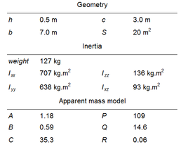
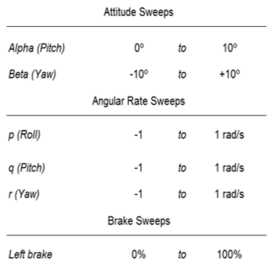
The analyses performed with the frozen equilibrium geometries are presented in Table 4. According to the linearized procedure assumed when running with the frozen geometry, the angle variations around the equilibrium positions are kept small. | The analyses performed with the frozen equilibrium geometries are presented in Table 4. According to the linearized procedure assumed when running with the frozen geometry, the angle variations around the equilibrium positions are kept small. | ||
| + | |||
<div class="center" style="width: auto; margin-left: auto; margin-right: auto;"> | <div class="center" style="width: auto; margin-left: auto; margin-right: auto;"> | ||
| − | + | [[File:Draft_Samper_447947970_3847_Table4.png|270px]] </div> | |
<div class="center" style="width: auto; margin-left: auto; margin-right: auto;"> | <div class="center" style="width: auto; margin-left: auto; margin-right: auto;"> | ||
| − | <span style="text-align: center; font-size: 75%;">Table 4: Runs computed for obtaining the aerodynamic derivatives.</span></div> | + | <span style="text-align: center; font-size: 75%;">'''Table 4''': Runs computed for obtaining the aerodynamic derivatives.</span></div> |
| + | |||
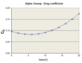
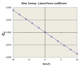
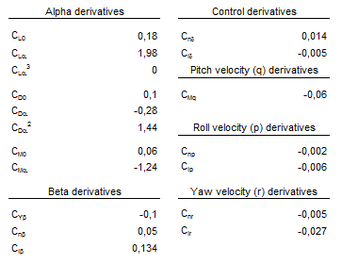
The aerodynamic derivatives are obtained from forces and moments data, computed at different flight conditions, by means of polynomial regression. Figure 12 shows a sample of the curves obtained for alpha and beta sweeps (pitch and yaw). The set of aerodynamic derivatives computed for the CIMSA parachute is presented in Table 5. | The aerodynamic derivatives are obtained from forces and moments data, computed at different flight conditions, by means of polynomial regression. Figure 12 shows a sample of the curves obtained for alpha and beta sweeps (pitch and yaw). The set of aerodynamic derivatives computed for the CIMSA parachute is presented in Table 5. | ||
| Line 434: | Line 521: | ||
| [[Image:draft_Samper_447947970-image87.png|center|282px]] | | [[Image:draft_Samper_447947970-image87.png|center|282px]] | ||
|} | |} | ||
| − | |||
| − | |||
| − | |||
{| | {| | ||
|- | |- | ||
| Line 445: | Line 529: | ||
<div class="center" style="width: auto; margin-left: auto; margin-right: auto;"> | <div class="center" style="width: auto; margin-left: auto; margin-right: auto;"> | ||
| − | <span style="text-align: center; font-size: 75%;">Figure 12: A sample of alpha and beta sweeps computed for the CIMSA parachute.</span></div> | + | <span style="text-align: center; font-size: 75%;">'''Figure 12''': A sample of alpha and beta sweeps computed for the CIMSA parachute.</span></div> |
| + | |||
<div class="center" style="width: auto; margin-left: auto; margin-right: auto;"> | <div class="center" style="width: auto; margin-left: auto; margin-right: auto;"> | ||
| Line 451: | Line 536: | ||
<div class="center" style="width: auto; margin-left: auto; margin-right: auto;"> | <div class="center" style="width: auto; margin-left: auto; margin-right: auto;"> | ||
| − | <span style="text-align: center; font-size: 75%;">Table 5: Estimated derivatives for the CIMSA parachute-payload system.</span></div> | + | <span style="text-align: center; font-size: 75%;">'''Table 5''': Estimated derivatives for the CIMSA parachute-payload system.</span></div> |
<span id='_Toc290547657'></span> | <span id='_Toc290547657'></span> | ||
| Line 458: | Line 543: | ||
The derivatives and inertial parameters listed in Tables 5 and 3 respectively are introduced in the dynamic simulator in order to perform trajectory and control analyses. In this example lateral and altitude control strategies are applied for the same payload drop conditions employed in the Application Example 1. The simulation results, though significantly different to that obtained for the Snowflake, are within normal expectations for a heavier parachute-payload system. It should be noticed that the performance for precision landing is heavily influenced by the control parameters; in this test case those listed in Table 6 are found to be acceptable although they could be further improved. | The derivatives and inertial parameters listed in Tables 5 and 3 respectively are introduced in the dynamic simulator in order to perform trajectory and control analyses. In this example lateral and altitude control strategies are applied for the same payload drop conditions employed in the Application Example 1. The simulation results, though significantly different to that obtained for the Snowflake, are within normal expectations for a heavier parachute-payload system. It should be noticed that the performance for precision landing is heavily influenced by the control parameters; in this test case those listed in Table 6 are found to be acceptable although they could be further improved. | ||
| + | |||
<div class="center" style="width: auto; margin-left: auto; margin-right: auto;"> | <div class="center" style="width: auto; margin-left: auto; margin-right: auto;"> | ||
| Line 463: | Line 549: | ||
<div class="center" style="width: auto; margin-left: auto; margin-right: auto;"> | <div class="center" style="width: auto; margin-left: auto; margin-right: auto;"> | ||
| − | <span style="text-align: center; font-size: 75%;">Figure 13: Trajectory plot computed for the CIMSA parachute-payload system.</span></div> | + | <span style="text-align: center; font-size: 75%;">'''Figure 13''': Trajectory plot computed for the CIMSA parachute-payload system.</span></div> |
| + | |||
<div class="center" style="width: auto; margin-left: auto; margin-right: auto;"> | <div class="center" style="width: auto; margin-left: auto; margin-right: auto;"> | ||
| Line 469: | Line 556: | ||
<div class="center" style="width: auto; margin-left: auto; margin-right: auto;"> | <div class="center" style="width: auto; margin-left: auto; margin-right: auto;"> | ||
| − | <span style="text-align: center; font-size: 75%;">Table 6: CIMSA parachute-payload system control parameters</span></div> | + | <span style="text-align: center; font-size: 75%;">'''Table 6''': CIMSA parachute-payload system control parameters</span></div> |
<span id='_Toc290547658'></span> | <span id='_Toc290547658'></span> | ||
| Line 478: | Line 565: | ||
The dynamic simulator presented in this work, together with the aerodynamic and structural tools developed by CIMNE, allow simulating the complete parachute-payload system, letting the designer to analyse design variations before building prototypes, the control system engineer to test different control strategies and the flight test engineer to predict the real performance of the system even before flying it once. In brief, involving simulation in the whole development process increases chances of success, shortening development time and costs. | The dynamic simulator presented in this work, together with the aerodynamic and structural tools developed by CIMNE, allow simulating the complete parachute-payload system, letting the designer to analyse design variations before building prototypes, the control system engineer to test different control strategies and the flight test engineer to predict the real performance of the system even before flying it once. In brief, involving simulation in the whole development process increases chances of success, shortening development time and costs. | ||
| + | |||
| + | ==Nomenclature== | ||
| + | |||
| + | a = height of the arc in the mid point | ||
| + | |||
| + | '''A, B, C''' = discrete linear model state-space matrices | ||
| + | |||
| + | A, B, C, P, Q, R, H = Lamb’s coefficients for apparent mass, inertia, and spanwise camber | ||
| + | |||
| + | AR = canopy aspect ratio | ||
| + | |||
| + | b = canopy span | ||
| + | |||
| + | C<sub>DS</sub> = payload drag coefficient | ||
| + | |||
| + | [[Image:draft_Samper_447947970-image1.png|6px]] = canopy mean chord | ||
| + | |||
| + | '''F'''<sub>W</sub> = weight vector in a body reference frame | ||
| + | |||
| + | '''F'''<sub>S</sub> = payload drag vector in a body reference frame | ||
| + | |||
| + | '''F'''<sub>A</sub>, '''M'''<sub>A</sub> = aerodynamic force and moment vectors in a body reference frame | ||
| + | |||
| + | '''F'''<sub>AM</sub>, '''M'''<sub>AM</sub> = apparent mass force and moment vectors in a body reference frame | ||
| + | |||
| + | H<sub>p</sub> = discrete model predictive controller prediction horizon | ||
| + | |||
| + | I<sub>T</sub> = inertia matrix of total system | ||
| + | |||
| + | I<sub>AM</sub>, I<sub>AI</sub> = apparent mass, inertia, and spanwise camber matrices | ||
| + | |||
| + | m = mass of the combined system including payload and canopy | ||
| + | |||
| + | [[Image:draft_Samper_447947970-image2.png|30px]] = angular velocity components in a body reference frame | ||
| + | |||
| + | [[Image:draft_Samper_447947970-image3.png|36px]] = angular velocity of the system in the canopy frame | ||
| + | |||
| + | [[Image:draft_Samper_447947970-image4.png|36px]] = cross-product matrix of the angular velocity expressed in a body and canopy reference frame | ||
| + | |||
| + | [[Image:draft_Samper_447947970-image5.png|30px]] = cross-product matrix of the vector from the mass centre to aerodynamic centre | ||
| + | |||
| + | [[Image:draft_Samper_447947970-image6.png|36px]] = cross-product matrix of the vector from the mass center to apparent mass center | ||
| + | |||
| + | [[Image:draft_Samper_447947970-image7.png|30px]] = cross-product matrix of the vector from the mass centre to canopy rotation point | ||
| + | |||
| + | [[Image:draft_Samper_447947970-image8.png|18px]] = cross-product matrix of the parafoil aerodynamic velocity | ||
| + | |||
| + | [[Image:draft_Samper_447947970-image9.png|36px]] = reference area of the parafoil canopy and payload | ||
| + | |||
| + | t = canopy mean thickness | ||
| + | |||
| + | T<sub>AC</sub> = transformation from aerodynamic to canopy frames | ||
| + | |||
| + | T<sub>BC</sub> = transformation from body to canopy frames | ||
| + | |||
| + | [[Image:draft_Samper_447947970-image10.png|30px]] = velocity components of mass centre in the body reference frame | ||
| + | |||
| + | [[Image:draft_Samper_447947970-image11.png|36px]] = velocity components of the aerodynamic centre in the canopy reference frame | ||
| + | |||
| + | [[Image:draft_Samper_447947970-image12.png|66px]] = aerodynamic velocities of the payload in the body frame | ||
| + | |||
| + | V<sub>Wind</sub> = velocity vector of the wind in an inertial reference frame | ||
| + | |||
| + | V<sub>A</sub>, V<sub>S</sub> = total aerodynamic speed of the parafoil canopy and payload | ||
| + | |||
| + | x, y, z = inertial positions of the system mass center | ||
| + | |||
| + | [[Image:draft_Samper_447947970-image13.png|12px]] = canopy incidence angle | ||
| + | |||
| + | [[Image:draft_Samper_447947970-image14.png|66px]] = distance vector components from mass centre to the canopy rotation point in a body ref frame | ||
| + | |||
| + | [[Image:draft_Samper_447947970-image15.png|72px]] = distance vector components from the canopy rotation point to the aerodynamic centre in a canopy reference frame | ||
| + | |||
| + | [[Image:draft_Samper_447947970-image16.png|36px]] = Euler roll, pitch, and yaw angles | ||
<span id='_Toc290547659'></span> | <span id='_Toc290547659'></span> | ||
Latest revision as of 12:50, 13 April 2018
1. Introduction
Gliding parachutes offer considerable scope for a large number of civil, humanitarian and military applications due to their ability to cover large horizontal distances from the drop point and their excellent controllability. A concept in the gliding-parachute category which has received attention since mid 60’s is the ram-air inflated fabric wing (also known as Jalbert parafoil or simply parafoil). Parafoils consist of a flexible fabric wing with rectangular planform and a streamlined cross-section which is opened at the leading edge to allow air to enter and inflate the wing to a specified shape. The payload is suspended on lines below the wing. Some of the earliest projects involving the usage of parafoil-based systems are discussed by Nikolaides and Knapp.1-7 and comprehensive bibliography up to 1980 is provided by Lingard8. Moreover, some definitions that in the last quarter of the twentieth century have become a sort of standard and discussion on modern parafoil design are given by Poynter9.
As it is possible to observe in the works mentioned above but also in more recent publications, parachute’s design and analysis rely mostly on empirical methods. An up-to-date example of this is a survey about the use of computational tools in the design and evaluation of parachute systems which was carried out with 15 worldwide parachute manufacturers10. All of ten responses received deny the employment of simulation software with the exception of computer assisted design (CAD) tools. This is a clear indication that, despite the growing relevance parachute systems have today in many application fields, computational mechanics is still hardly applied to their design and analysis.
With the objective of addressing this shortcoming, a series of computational tools have been developed at CIMNE in recent times. Most of them are integrated in a simulation code intended for the unsteady simulation of ram-air type parachute-payload systems11 which is based on an unsteady low-order panel method12 coupled with a membrane finite element explicit technique13 (including cords and ribbons models). In addition, the development of a set of complementary tools aimed at studying in an integrated manner the flight performance of guided parafoil-payload systems was undertaken. This software package consists of a 6 degree-of-freedom (DoF) dynamic simulator, based on aerodynamic derivatives, and an autonomous guidance, navigation and control system (GNC) implemented by means of a proportional-integral-derivative (PID) algorithm. Briefly, dynamic models based on derivatives offer a simple mathematical way of describing the flight dynamics of an aerodynamic system by means of linearized equations written in terms of suitable non-dimensional (constant) coefficients known as aerodynamic derivatives. These coefficients, which define, for example, how the aerodynamic forces and moments change with the angle of attack, yaw or brake deflections, determine the response of the system to small deviations from the equilibrium conditions at which it is linearized. The fidelity of the model depends on the number and accuracy of the derivatives employed. In this way, the behaviour of a particular parafoil-payload system can be modelled up to a desired degree of fidelity by defining a proper set of aerodynamic derivatives and also mass and inertial parameters. Given these characteristics through experimental or numerical means, the model allows predicting the behaviour of the system subject to different flight and environmental conditions with a very low computational cost, making feasible parachute and mission real-time analyses. The main aspects underlying the 6-DoF simulator and the GNC model are described in this document.
The work is organized as follows. Section 2 briefly reviews some of the most important experiences in the modelling of parafoil vehicles. The 6 DoF dynamic model and the GNC strategy implemented are presented in Sections 3 and 4 and a first application example is provided in Section 5. Next, an advanced procedure for estimating aerodynamic derivatives from numerical data computed with CIMNE’s parachute code11 is presented in Section 6 and an application test case is given in Section 7. Finally, some relevant conclusions and future lines of research are drawn in Section 8. Moreover, with the objective of summarizing current airdrop technology, some of the most relevant parafoil systems are described in Appendix A at the end of this document.
2. Modelling historic background
Since the introduction of ram-air parafoils in the mid 60’s numerous experimental and numerical studies were carried out to model their behaviour and predict in-flight performance. In the next, a few of the most important milestones in parafoil modelling are highlighted; cf. Yakimenko14 for a detailed review.
Even though parafoils belong to the parachute family, in the air they behave like an aircraft, but at significantly lower speeds. Since these kinds of low-speed aerodynamics problems were not studied enough when parafoils appeared, the need to carry out new investigations was clear. Nikolaides et al.1,2 conducted the first wind-tunnel and free-flight tests of a ram-air wing at the University of Notre Dame in 1964and, some years later, Burk et al.15 performed similar tests at the NASA Langley Research Center. These experiments confirmed that parafoils have airplane-wing behaviour but with gentle stall characteristics, consequence of their flexible structure. Due to the advantages over classical round parachutes, in the late 80’s the ram-air parafoil configuration was chosen for the Advanced Recovery Systems (ARS) for the Next Generation Space Transportation System16,17. The full scale prototype (10,800ft2) was tested at NASA Ames Research Center9 and, later, a flight test campaign was also conducted.
Besides experimental efforts, the numerical modelling of parafoil-payload systems started in the late 70’s. For over a decade, 3 and 4-DoF models were developed to analyze both static and dynamic longitudinal stability of high-performance airdrop systems18-23. Among other important results, these studies showed that the optimum performance for a conventional ram-air parachute is close to 3:1 and the gliding efficiency is strongly influenced by the position of the suspended load under the canopy. Later, other studies highlighted the need to include apparent mass effects in the models in order to achieve more reliable simulations. This issue was firstly addressed by Lissaman and Brown in the early 90`s by modelling the parachute as an ellipsoid24. By the end of that decade, the interest in using parafoil-payload systems for defence purposes led to the development and employment of higher fidelity models using 6, 9, 10 and even 15 DoFs to model the flight mechanics of the system. As might be expected, the coefficients provided by experimental and numerical means were not enough for these sophisticated models. This fact promoted advanced experimental studies and the development of a new generation of simulation tools based on reduced-order computational aerodynamics models and computational fluid dynamics (CFD) techniques (mainly driven by the rapid growing of computer power). As mentioned in the introduction to this work, even though it is possible to say that such techniques are mature and its employment is usual in many engineering fields, very little progress has been made in parachute simulation and this is currently a field of active research. The high complexity of the aero-structural problems involved in parachute simulation could explain the lack of numerical applications to a large extent.
3. Parafoil dynamic model
Although the range of possibilities between the early 2 or 3-DoF models and the most sophisticated 15-DoF models is extensive, the literature shows that current practical applications rely, in general, on 6 or 9-DoF models, depending on whether independent payload rotation is considered or not. The fact that simple 6-DoF models have been successfully used in the past with very good agreement with experimental data (provided that the model is properly tuned25) motivates its adoption in this project. It was also considered that, if needed in future applications, its expansion to 9 DoF is straightforward.
The 6 DoF parafoil dynamic model adopted in this work follows the general lines given by Slegers et al.26. Because of the complexity of the parafoil-payload system, it is advantageous to make certain simplifications to the model so that simulation and control analysis are more straightforward. One such simplification is to assume that the entire parafoil-payload system behaves as a rigid body once it is completely inflated, thus, the treatment is like a conventional aircraft with the wing positioned high above the fuselage. Figure 1 sketches the parafoil-payload system and the coordinate’s frames employed. The model considers three inertial position components of the total system mass centre as well as three Euler orientation angles. The incidence angle Γ defines the relative angle between the canopy and the payload and is considered a pilot input. Three characteristic points are defined: the aerodynamic centre of the canopy (P), the apparent mass centre (M) and the canopy rotation centre (C), which depends on the incidence angle.
The kinematic of the parafoil-payload system can be defined by

|
(1) |

|
(2) |
where TIB is the transformation matrix from an inertial reference frame to the body reference frame

|
(3) |
The equations of motion of the parachute-payload system can be obtained by summing up forces and moment contributions about the system centre of gravity (CG). Thus,
| (4) |
| (5) |
The following convention is used for the vector cross product of two vectors r = {rx ry rz}T and F = {Fx Fy Fz}T both expressed in the aerodynamic reference frame

|
(6) |
The forces appearing in Eq. (4) are the weight (FW), the canopy aerodynamic load (FA), the payload aerodynamic load (FS) and the apparent mass forces (FAM). These contributions are developed in the following equations.
Starting with the weight contribution, we can define

|
(7) |
Then, before defining aerodynamic forces, the aerodynamic velocities and angles are written in terms of the wind components and the canopy relative angle of incidence. Thus,

|
(8) |
| |
(9) |
| |
(10) |
| |
(11) |
where the transformation from body to canopy reference frames can be expressed by

|
(12) |
The aerodynamic force is defined in terms of aerodynamic derivatives (these are considered known data). Thus,

|
(13) |
with TAB being the transformation from the aerodynamic to canopy reference frame

|
(14) |
The only force taken into account for the payload is the drag. This is expressed in terms of its own local velocity (in the body reference frame) by

|
(15) |
Besides the forces contribution to the total system moment, there are two additional terms in Eq. (5) that correspond to aerodynamic and apparent mass moments. Similar to the aerodynamic forces, the aerodynamic moment is defined in terms of derivatives

|
(16) |
As the parafoil moves through the air, it displaces and accelerates the fluid surrounding it. The apparent mass effect is defined as the reaction of the fluid surrounding the parafoil. In high mass-to-volume ratio bodies like airplanes this reaction is negligible, but in very light vehicles like parafoils it plays an important role and can significantly affect their behaviour. A common practice is to add this effect as additional mass and inertia terms named “apparent mass” and “apparent inertia” which can be derived from the total kinetic energy of the fluid set in motion along with the parafoil. According to Lamb27, the kinetic energy can be expressed for a typical parachute canopy having two planes of symmetry, x-z and y-z, by
| |
(17) |
where the seven constants are defined in terms of parachute geometric parameters. In addition, if we neglect the spanwise camber effect, the constant H can be considered to be zero (this is the approach adopted here). Therefore, using the formulae given by Lissaman and Brown24, the apparent mass terms A, B, C, P, Q and R can be computed as follows

|
(18) |

|
(19) |

|
(20) |
| |
(21) |
| (22) |

|
(23) |
Then, forces and moments due to apparent mass and inertia can be obtained by relating the momentum of the fluid surrounding the parafoil to its kinetic energy. Following Lissman and Brown,

|
(24) |

|
(25) |

|
(26) |

|
(27) |
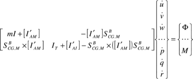
Finally, the set of dynamic equations of motion is obtained by replacing all the previous forces and moments into Eqs. (4) and (5). Thus,
|
(28) |

|
(29) |

|
(30) |
where the following notation applies
| (31) |
In the matrix in Eq. (29) it is possible to observe that apparent mass effects couple linear and rotational dynamics, which would be decoupled otherwise (in models where apparent mass coefficients are constant).
4. Automatic Control Strategy
Autonomous parafoil systems are designed to guide the flight from an arbitrary release point towards a desired landing point by means of an on-board computer, sensors and actuators. These components and their control algorithms constitute the so-called guidance, navigation and control system (GNC). The navigation subsystem manages data acquisition, processes sensor data and provides guidance and control subsystems with information about parafoil state (attitude). Using this information along with other available system data (such as local wind profiles), the guidance subsystem computes a feasible (physically realizable and mission compatible) trajectory from the initial position to the desired landing point. Finally, it is the responsibility of the control system to track this trajectory using the information provided by the navigation subsystem and on-board actuators. The GNC technique implemented in this work is intended to demonstrate the simulator’s flexibility and potential for its use in the design and evaluation of control algorithms.
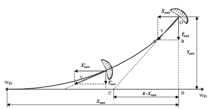
The heading tracking technique described below is based on Niculescu’s28 implementation for the PID navigation system of the Aerosonde UAV, currently considered one of the most advanced unmanned aerial vehicles (UAVs). Accordingly, lateral track control is employed in the present work for guiding the parachute from a waypoint W p1 (parachute deployment) to a specified target waypoint W p2 through a yaw-rate command (see Figure 2).
The control strategy proceeds as follows. For a given parachute track position , measured from W p2, the vehicle ground velocity vector is pointed in the direction of a line intercepting the track at point C. The interception point C is determined by considering that the distance on the track line from this point to Wp2 is, at any instant time, equal to , being k a design parameter. From the geometry of the similar triangles OAB and OCD, the parachute position and velocity is established according to
| (32) |
Accordingly, an error E is defined by
| (33) |
If Eq. (33) is not satisfied (meaning that there is a heading error), the magnitude and sign of error E is used to define a parachute brake command. This is done in two steps: first a “desired yaw-rate” is defined and then parachute brakes are pulled in order to obtain it. The “desired yaw-rate” is defined as follows,
| (34) |
where the proportional gain should be determined iteratively in order to achieve good tracking without overshoots. Moreover, the yaw-rate is limited to rad/s with the aim of avoiding numerical misbehaviours. To command the parachute, brakes are actuated by comparison of the “desired yaw-rate” with the actual yaw-rate. If there is a difference, a brake input is generated left or right, depending on the sign resulting from the comparison. This process is summarized in the following expression,
| |
(35) |
where is a constant taking into account the kinematics of the parachute brake line.
Altitude Control
Parafoil altitude control deals with potential energy management. The altitude control strategy adopted in this work divides the parafoil flight in three parts: an initial straight down gliding phase followed by a spiral descent phase and a final straight down approach towards the target. The first phase begins immediately after the parachute is deployed and extends until the target distance is reduced by a specified percentage. During this phase the parafoil uses only lateral control to navigate to the target and the travelled distance is recorded in order to evaluate an average parachute glide slope. At the beginning of the second phase, the control system computes an “ideal” flight altitude (hideal) according to
| |
(36) |
where Dtarget is the remaining distance to target and GSPhase_1 is the average glideslope measured at the initial phase. If the real parachute altitude hreal is greater than hideal, a spiral descent is initiated by a specified constant brake input which holds until hreal < hideal. Otherwise, the descent is omitted because the parachute altitude could be insufficient to reach the target. The third flight phase begins when hreal ≤ hideal and involves the final approach. During this stage both lateral and glideslope controls are applied. The latter is implemented through a variable incidence angle which is determined by the following proportional control
| |
(37) |
where kp is the proportional gain. The incidence angle is increased (to the negative side) if the parafoil is higher than hideal and decreased in the opposite case. This allows achieving a very fine adjustment of the glide slope as the parachute approaches to the target.
5. Application example 1. Snowflake test model
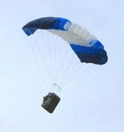
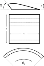
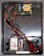
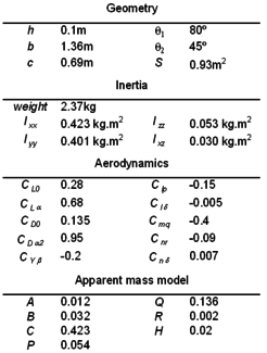
Snowflake is a small parafoil-payload system employed in an on-going research project between the U.S. Navy Postgraduate School and the University of Alabama in Huntsville. The main objective of the project, which is funded by the U.S Army Special Operations Command, is the development of a precision airdrop system intended to evaluate advanced concepts in controlling single and multiple (during mass airdrop) guided autonomous parafoils. The main characteristics1 of the Snowflake parafoil are summarized in Table 1.
(1) It must be noticed that the data was provided by Prof. Slegers from the University of Alabama in a personal communication to the authors
Simulation Results
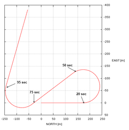
This initial test is intended to examine the basic capabilities of the simulator. The parachute-payload system is deployed at 500m altitude with heading north, fixed incidence angle Γ = -12º and no wind. Left brake input is applied 20 seconds after deployment and held during 30 seconds. Later, 75 seconds from deployment, right brake input is applied during 20 seconds. The trajectory computed by the simulator is presented in Figure 4.
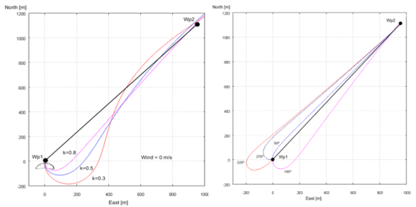
Next, the performance of the control algorithm is assessed by guiding the parachute-payload system through a flight path defined by waypoints W p1 and W p2. Figure 5 shows three flight paths computed for different values of design parameter k and heading angles.
Figure 5. Left: influence of the design parameter k on the guided trajectory for a South release heading (180º). Right: automatic control response to different release heading angles (k = 0.8).
Figure 5 (left) shows that the trajectory is noticeably affected by the design parameter k; in the present example smaller values of k lead to a faster track interception but with a considerable overshoot. Therefore, this parameter should be adjusted depending on the mission requirements As regards initial heading, Figure 5 (right) demonstrates that it is successfully managed by the control system even under the most adverse release conditions.
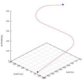
The second test applies full lateral and altitude control to a typical payload drop. The system is deployed at 2000 meters of altitude, 2200 meters away from the target, with wind coming from the south at 3 meters per second. Initially, the system navigates directly to the target regardless of the excess of altitude (Phase 1). When the horizontal distance to the target is reduced by 75% and spiral descent is performed until reaching hideal (Phase 2). At this point, navigation to the target is re-engaged and glideslope control is activated (incidence angle variation, Phase 3). The computed trajectory is depicted in Figures 6 and 7. It should be noticed that although the parafoil touchdown took place at an acceptable distance from the target (74 meters), the precision could be further improved by fine tuning of the control gains. The gain parameters used in this simulation are presented in Table 2.
Finally, a similar test case is solved but this time considering wind effects. The simulation results are shown in Figure 8, where it can be observed that the control system has a very good performance in the no-wind condition but deteriorates with wing, a situation in which a strong dependance on its intensity and direction is identified. This behavior can be enhanced by taking into account wind conditions and relative position of the parafoil with respect to the target when the switch from flight phase 2 to phase 3 is computed. These strategies are currently a topic of investigation of many research groups, cf. Yakimenko29 for an overview.
6. Advanced aerodynamic parameters estimation
Although coupling trajectory analysis tools with realistic CFD simulations is today a topic under intensive research30-31, practical applications require keeping analysis time and computational requirements as small as possible and this fact motivated the derivatives based dynamic model adopted in this work. In spite of the fact that these models are simple to implement and have a very low computational cost, the accurate definition of the aerodynamic derivatives, mass and inertial parameters which model the dynamics of the system is not a trivial task. While mass and inertial parameters are easier to compute (they depend on geometrical design and materials properties), the aerodynamic derivatives should be estimated through experimental and/or numerical means. Although the most accurate way is the experimental one, the experiments are expensive and very time consuming. Therefore, the numerical simulation becomes an attractive alternative approach to compute the derivatives (at the expense of accuracy and results scope). The work developed in the next aims at exploring the capabilities of CIMNE’s simulation software11 to characterize the aerodynamic behaviour of a parachute-payload system.
Derivatives Estimation Procedure
In spite of the fact that no universal procedure exists for computing aerodynamic derivatives, generally these are estimated from the analysis of the aerodynamic forces and moments resulting at different body attitudes and flight conditions. It should be noticed that, contrary to rigid bodies for which the shape is well determined and a certain attitude for analysis is set straightforward, determining the exact attitude and shape of a parachute is a complex task. Due to its flexible structure, for a given release condition the flight attitude of a parachute depends on its deformed shape, mass and inertial parameters. In addition, the deformed shape of the parachute will depend on the resulting set of loads acting on it, which, in turn, depend on the attitude and flight conditions. Therefore, the shape and attitude of a parachute cannot be specified a-priori like it occurs with rigid bodies. To work out this situation it was decided to perform the runs needed to compute the derivatives with a frozen parachute equilibrium configuration obtained from simulation. With this aim, the coupled computation is started with a given parachute geometry and attitude (resulting from release conditions) and ran until the parachute reaches a stable flight and acquires its equilibrium deformed shape. The latter geometry can be used to compute the derivatives as long as the analysis angles do not deviate too far from the equilibrium position. Notice that this linearized procedure is in agreement with the concepts underlying derivative models and do not impose any restrictions on the analysis beyond those due to the potential flow model adopted.
Once the parachute equilibrium geometry is obtained, fixed-angle and angular rate sweeps are performed to compute the aerodynamic derivatives. The fixed angle calculations are aimed at obtaining stationary aerodynamic characteristics for different angles of attack (alpha), yaw (beta) and brake deflections (delta). The angular rate derivatives are obtained by setting fixed angular velocities about the body axes, one at a time. Finally, the control system derivatives are obtained by unsymmetrically deflecting the brake at different positions. The procedure employed to obtain the equilibrium configuration with brakes deflected is similar to that explained before, but this time the brake is pulled a desired distance after equilibrium flight is achieved. The very short unsteady phase occurring immediately once the brake is pulled is omitted and the equilibrium shape for each brake deflection is used to execute the fixed angle and rate sweeps needed for computing the control derivatives. To avoid instabilities and parachute behaviours out of the scope of the potential flow assumptions, this calculation is performed only at small angles of attack. As regards the viscous contributions to the aerodynamic forces and moments, e.g. suspension lines drag, these are estimated by semi-empirical methods and added to the inviscid results given by the simulation code.
7. Application example 2. CIMSA test model
In this numerical application aerodynamics derivatives are computed for a small parachute-payload system by applying the procedure described in the previous section. The parachute, which is provided by provided by CIMSA Ingeniería en Sistemas32, is solved with the coupled code for a given initial shape and release conditions to obtain the inflated flight equilibrium geometry. This geometry is then frozen and used as a rigid body to perform the required pitch, roll, yaw and angular rate sweeps. Figure 11 shows deformed equilibrium geometries of the parafoil obtained for stable flight with and without brake deflection. The payload mass and inertia are reproduced by a proper adjustment of the material properties of the triangle suspended below the canopy. The main characteristics of the parachute-payload system are listed in Table 3.
The analyses performed with the frozen equilibrium geometries are presented in Table 4. According to the linearized procedure assumed when running with the frozen geometry, the angle variations around the equilibrium positions are kept small.
The aerodynamic derivatives are obtained from forces and moments data, computed at different flight conditions, by means of polynomial regression. Figure 12 shows a sample of the curves obtained for alpha and beta sweeps (pitch and yaw). The set of aerodynamic derivatives computed for the CIMSA parachute is presented in Table 5.
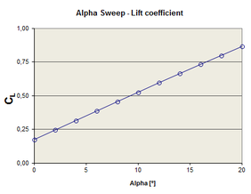
|
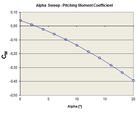
|
Simulation Results
The derivatives and inertial parameters listed in Tables 5 and 3 respectively are introduced in the dynamic simulator in order to perform trajectory and control analyses. In this example lateral and altitude control strategies are applied for the same payload drop conditions employed in the Application Example 1. The simulation results, though significantly different to that obtained for the Snowflake, are within normal expectations for a heavier parachute-payload system. It should be noticed that the performance for precision landing is heavily influenced by the control parameters; in this test case those listed in Table 6 are found to be acceptable although they could be further improved.
8. Conclusions
The role parachutes have in many civil, humanitarian and military applications call for new and improved computational tools aimed at tackling the current lack of software applications in the field. The present project, which is part of a research line being developed at CIMNE for these purposes, involves the development of numerical tools for the analysis and evaluation of autonomous parafoil systems. These tools, which are based on a 6-DOF dynamic parachute model and a GNC system implemented by means of PID algorithms, facilitate the user to test designs, develop and evaluate control strategies and analyze real-life drop scenarios. As an example of potential use, lateral and altitude control strategies were successfully developed and tested. Future implementations will include Monte Carlo simulations for statistical analysis of landing precision, parameter identification for flight-tests data reduction and an advanced GUI.
The dynamic simulator presented in this work, together with the aerodynamic and structural tools developed by CIMNE, allow simulating the complete parachute-payload system, letting the designer to analyse design variations before building prototypes, the control system engineer to test different control strategies and the flight test engineer to predict the real performance of the system even before flying it once. In brief, involving simulation in the whole development process increases chances of success, shortening development time and costs.
Nomenclature
a = height of the arc in the mid point
A, B, C = discrete linear model state-space matrices
A, B, C, P, Q, R, H = Lamb’s coefficients for apparent mass, inertia, and spanwise camber
AR = canopy aspect ratio
b = canopy span
CDS = payload drag coefficient
= canopy mean chord
FW = weight vector in a body reference frame
FS = payload drag vector in a body reference frame
FA, MA = aerodynamic force and moment vectors in a body reference frame
FAM, MAM = apparent mass force and moment vectors in a body reference frame
Hp = discrete model predictive controller prediction horizon
IT = inertia matrix of total system
IAM, IAI = apparent mass, inertia, and spanwise camber matrices
m = mass of the combined system including payload and canopy
= angular velocity components in a body reference frame
= angular velocity of the system in the canopy frame
= cross-product matrix of the angular velocity expressed in a body and canopy reference frame
= cross-product matrix of the vector from the mass centre to aerodynamic centre
= cross-product matrix of the vector from the mass center to apparent mass center
= cross-product matrix of the vector from the mass centre to canopy rotation point
= cross-product matrix of the parafoil aerodynamic velocity
= reference area of the parafoil canopy and payload
t = canopy mean thickness
TAC = transformation from aerodynamic to canopy frames
TBC = transformation from body to canopy frames
= velocity components of mass centre in the body reference frame
= velocity components of the aerodynamic centre in the canopy reference frame
= aerodynamic velocities of the payload in the body frame
VWind = velocity vector of the wind in an inertial reference frame
VA, VS = total aerodynamic speed of the parafoil canopy and payload
x, y, z = inertial positions of the system mass center
= canopy incidence angle
= distance vector components from mass centre to the canopy rotation point in a body ref frame
= distance vector components from the canopy rotation point to the aerodynamic centre in a canopy reference frame
= Euler roll, pitch, and yaw angles
Acknowledgments
The authors wish to acknowledge the contribution of Prof. Sleegers from the University of Alabama in Huntsville who kindly provided the experimental data concerning the Snowflake parafoil. Thanks are also given to CIMSA for providing the parachute geometry employed to test the advanced derivatives estimation procedure and also to Mr. Boris Hahn for helping with the simulation runs required to extract these data. Last but not least, the financial support of the CIMNE Foundation for Latin-America is also gratefully acknowledged.
References
1 Nicolaides, J.D., Knapp, C.F., “A Preliminary Study of the Aerodynamic and Flight Performance of the Parafoil,” AIAA Paper 1965, 1st AIAA Conference on Aerodynamic Decelerator Systems, University of Minnesota, MN, July 8, 1965.
2 Nicolaides, J.D., “On the Discovery and Research of the Parafoil,” International Congress on Air Technology, Little Rock, AK, 1965.
3 Knapp, C.F., Barton, W.R., “Controlled recovery of Payloads at Large Glide Distances, Using the Para-Foil,” Journal of Aircraft, 5(2), 1968.
4 Nicolaides, J.D., Speelman, R.J., Menard, G.L.C., “A Review of Para-Foil Programs,” AIAA Paper 1968, 2nd AIAA ADS Conference, El Centro, CA, September 23-25, 1968.
5 Nicolaides, J.D., “Improved Aeronautical Efficiency Through Packable Weightless Wings,” AIAA Paper 1970-880, CASI/AIAA Meeting on the Prospects for Improvement in Efficiency of Flight, Toronto, Canada, July 9-10, 1970.
6 Nicolaides, J.D., Speelman, R.J., Menard, G.L.C., “A Review of Para-Foil Applications,” Journal of Aircraft, 7(5), 1970.
7 Nicolaides, J.D., Tragarz, M.A., “Parafoil flight performance,” AIAA Paper 1970-1190, 3rd AIAA ADS Conference, Dayton, OH, September, 14-16, 1970.
8 Lingard, J.S., “The Performance and Design of Ram-Air Parachutes,” TR-81-103, UK Royal Aircraft Establishment, Farnborough, 1981.
9 Poynter, D., The Parachute Manual. A Technical Treatise on Aerodynamic Decelerators, Vol.2, 1991.
10 Guerra, A. “Development and validation of a numerical code for analysing parachutes”. Undergraduated thesis presented at the Scola Tecnica Superior d'Enginyers Industrial i Aeronàutica de Terrassa, Technical University of Catalonia (in Spanish), 2009.
11 Ortega, E., Flores, R., Oñate, E., Sacco, C., González, E., Innovative Numerical Tools for the Simulation of Parachutes, CIMNE Research Publication PI 341, 2010.
12 Ortega, E., Flores, R., and Oñate, E. A 3D low-order panel method for unsteady aerodynamic problems. CIMNE Research Publication PI 343, 2010.
13 Flores, R., Ortega, E., and Oñate, E. Explicit dynamic analysis of thin membrane structures CIMNE Research Publication PI 351, 2010.
14 Yakimenko, O.A., “On the Development of a Scalable 8-DoF Model for Generic Parafoil-Payload Delivery System”, Proc. of the 18th AIAA Aerodynamic Decelerator Systems Technology Conference and Seminar, Munich, Germany, May 24-26, AIAA 2005-1665, 2005.
15 Burk, S.M., Ware, G.M., Static Aerodynamic Characteristics of Three Ram-Air Inflated Low Aspect Ratio Fabric Wings, TND-4182, NASA, 1967.
16 Wailes, W.K., “Advanced Recovery Systems for Advanced Launch Vehicles (ARS). Phase 1 Study Results,” AIAA Paper 1989-0881, 10th AIAA ADST Conference, Cocoa Beach, FL, April 18-20, 1989.
17 Wailes, W.K., “Development testing of large ram air inflated wings,” AIAA Paper 1993-1204, 12th RAeS/AIAA ADST Conference and Seminar, London, England, May 10-13, 1993.
18 Goodrick, T.F., “Theoretical study of the longitudinal stability of high-performance gliding airdrop systems,” AIAA Paper 1975-1394, 5th AIAA ADS Conference, Albuquerque, NM, November 17-19, 1975.
19 Goodrick, T.F., “Simulation studies of the flight dynamics of gliding parachute systems,” AIAA Paper 1979-0417, 6th AIAA AD and Balloon Technology Conference, Houston, TX, March 5-7, 1979.
20 Goodrick, T.F., “Comparison of simulation and experimental data for a gliding parachute in dynamic flight,” AIAA Paper 1981-1924, 7th AIAA ADBT Conference, San Diego, CA, October 21-23, 1981.
21 Crimi, P., “Lateral Stability of Gliding Parachutes,” Journal of Guidance, Control Dynamics, 13(6), 1990.
22 Iosilevskii, G., “Center of Gravity and Minimal Lift Coefficient Limits of a Gliding Parachute,” Journal of Aircraft, 32(6), 1995, pp.1297-1302.
23 Jann, T., “Aerodynamic model identification and GNC design for the parafoil-load system ALEX,” AIAA Paper 2001-2015, 16th AIAA ADST Conference and Seminar, Boston, MA, May 21-24, 2001.
24 Lissaman, P.B.S., Brown, G.J., “Apparent mass effects on parafoil dynamics,” AIAA Paper 1993-1236, 12th RAeS/AIAA ADS Technology Conference, London, England, May 10-13, 1993.
25 Mortaloni, P., Yakimenko, O., Dobrokhodov, V., and Howard, R., “On the Development of a Six-Degree-of-Freedom Model of a Low-Aspect-Ratio Parafoil Delivery System,” 17th AIAA Aerodynamic Decelerator Systems Technology Conference and Seminar, Monterey, CA, May 19-22, 2003.
26 Slegers, N., Costello, M., Beyer, E., “Use of Variable Incidence Angle for Glide Slope Control of Autonomous Parafoils,” Journal of Guidance, Control Dynamics, 31(3), 2008.
27 Lamb, H., “Hydrodynamics”, Dover, New York, 1945, pp. 160-174.
28 Niculescu, M., “Lateral Track Control Law for Aerosonde UAV”, AIAA 2001-0016, 2001.
29 Yakimenko O., Slegers N., “Using direct methods for terminal guidance of autonomous aerial delivery systems”, Proceedings of the European Control Conference 2009, Budapest, Hungary, August 2009.
30 T.E. Tezduyar, “Finite Element Methods for Flow Problems with Moving Boundaries and Interfaces,” Archives of Computational Methods in Eng., vol. 8, 2001, pp. 83–130.
31 K. Stein, T. Tezduyar, and R. Benney, “Applications in Airdrop Systems: Fluid-Structure Interaction Modeling,” Proc. 5th World Congress on Computational Mechanics, Vienna Univ. of Technology, Austria, 2002.
32 CIMSA Ingeniería en Sistemas. Web page: http://www.cimsa.com/ (13 April 2011)
Appendix A: Current precision airdrop systems
Although parafoil systems are more expensive than round parachutes, they offer important advantages such as higher glide ratios and an improved manoeuvrability, which allows achieving higher precision at the landing point. In addition to research at universities, several companies have already developed commercial products in the format of “Precision Aerial Delivery Systems” which aim directly to the defence market.
The U.S. government has developed a program called Joint Precision Airdrop System (JPADS) that combines the U.S. Army's Precision and Extended Glide Airdrop System (PEGASYS) program with the U.S. Air Force's Precision Airdrop System (PADS) program to meet joint requirements for precision airdrop. JPADS involves four increments, categorized by the weight of the cargo to be dropped:
- Increment I: JPADS-2K / applies to loads up to 2,200 lbs / classified as the “extra light” category / commensurate with Container Delivery System (CDS) bundles.
- Increment II: JPADS-10K / applies to loads up to 10,000 lbs.
- Increment III: JPADS-30K / applies to loads up to 30,000 lbs.
- Increment IV: JPADS-60K / applies to loads up to 60,000 lbs.
Many companies have developed products that fulfil the precision airdrop requirements under the JPADS program. One of the leader companies is Atair Aerospace, Inc. with the Onyx family, capable of payload deliveries from 10 to 2200 pounds. The company claims that the “Onyx systems are air-deployed from military fixed-wing and rotary aircraft (A/C), such as a C-130 or C-17, at altitudes up to 35,000 ft and speeds up to 150 KIAS, autonomously glide over 40 km, and land cargo within a circular error probability (CEP) of 100 m”. Some of their designs are hybrid round/ram-air parachutes, as shown in Figure A-1. Every system includes adaptive control, intelligent collision avoidance and a complete base station.
Another leading company offering products under the JPADS program is Airborne Systems. They have developed systems that can deliver payloads from 100 to 42,000 lbs. and claim that they have “increased payload survivability due to the system’s unique ability to perform a flared into-the-wind landing”.
|
These and other companies are also offering the avionics system to be adapted to customer parachute systems. This is the case, for example, of Capewell Components Company LLC, which is offering a so-called Universal Precision Airdrop System that “is designed to accommodate a range of small to medium payload sizes and can use either round G-12 or ram air parafoil parachutes interchangeably”. Thus, it has the versatility to be used with a variety of parachute and pallet systems.
STARA is another company developing airdrop systems that has been awarded with a contract to develop a system for delivering medical supplies. This may be used not only in battlefields but also in a natural disaster scenario. Their system is called Mosquito and is capable of delivering payloads up to 150 pounds within 30 meters of accuracy.
Document information
Published on 01/01/2011
Licence: CC BY-NC-SA license
Share this document
Keywords
claim authorship
Are you one of the authors of this document?


