| (48 intermediate revisions by 3 users not shown) | |||
| Line 2: | Line 2: | ||
| − | ===Aeroelasticity Analysis of Folding | + | ===Aeroelasticity Analysis of Folding Wing with Structural Nonlinearity Using Modified DLM=== |
<div class="center" style="width: auto; margin-left: auto; margin-right: auto;"> | <div class="center" style="width: auto; margin-left: auto; margin-right: auto;"> | ||
| Line 16: | Line 16: | ||
Correspondence: [mailto:ygni.good@163.com ygni.good@163.com]</div> | Correspondence: [mailto:ygni.good@163.com ygni.good@163.com]</div> | ||
--> | --> | ||
| − | + | ==Abstract== | |
| − | ==Abstract | + | |
The structural nonlinear aeroelastic analysis of folding wings is conducted by integrating the modified Doublet Lattice Method in this paper. Firstly, a modified Doublet Lattice Method is investigated to relax the aspect ratio limitation of aerodynamic elements, and its correctness is verified through numerical examples. Secondly, the rational function approximation method is discussed, and the modified Doublet Lattice Method is approximated using the minimum state method to obtain the unsteady aerodynamic forces in the time domain. Finally, the aeroelastic characteristics of a folding wing with free-play and friction nonlinearity are studied by integrating time-domain unsteady aerodynamics with the nonlinear structural dynamics model. The results show that the modified Doublet Lattice Method, which relaxes the aspect ratio limitation of aerodynamic grid elements, is feasible and effective; Friction can suppress the influence of free-play nonlinearity on aeroelastic response. | The structural nonlinear aeroelastic analysis of folding wings is conducted by integrating the modified Doublet Lattice Method in this paper. Firstly, a modified Doublet Lattice Method is investigated to relax the aspect ratio limitation of aerodynamic elements, and its correctness is verified through numerical examples. Secondly, the rational function approximation method is discussed, and the modified Doublet Lattice Method is approximated using the minimum state method to obtain the unsteady aerodynamic forces in the time domain. Finally, the aeroelastic characteristics of a folding wing with free-play and friction nonlinearity are studied by integrating time-domain unsteady aerodynamics with the nonlinear structural dynamics model. The results show that the modified Doublet Lattice Method, which relaxes the aspect ratio limitation of aerodynamic grid elements, is feasible and effective; Friction can suppress the influence of free-play nonlinearity on aeroelastic response. | ||
| − | ''' | + | '''Keywords''': Folding wing, modified doublet lattice method, rational function approximation, structural nonlinearity |
| − | == | + | ==1. Introduction== |
With the complexity of aircraft flight missions, the ability to adapt to multiple tasks and achieving “one aircraft with multiple capabilities” has gradually become a new requirement for aircraft design. As a result, morphing aircrafts that can change the shape of aircraft to adapt to different flight environments, improve aerodynamic performance, and expand flight envelopes have emerged, and have shown broad application prospects in the aviation field [1]. At present, the morphing mode that has been extensively studied is still folding wings [2]. | With the complexity of aircraft flight missions, the ability to adapt to multiple tasks and achieving “one aircraft with multiple capabilities” has gradually become a new requirement for aircraft design. As a result, morphing aircrafts that can change the shape of aircraft to adapt to different flight environments, improve aerodynamic performance, and expand flight envelopes have emerged, and have shown broad application prospects in the aviation field [1]. At present, the morphing mode that has been extensively studied is still folding wings [2]. | ||
| − | Snyder et al. analyzed the vibration and flutter characteristics of the folding wing configuration [3]. Wang et al. conducted relevant research on the aeroelasticity and structural mechanics of folding wing models [4]. Lee et al. utilized MSC.NASTRAN and ZEARO software to analyze the relationship between flutter and folding angle [5], and further conducted structural nonlinear aeroelastic analysis [6]. Attar et al. conducted theoretical analysis and experimental verification on the nonlinear aeroelastic response of the folding wing structures [7]. Reich et al. analyzed and studied the aeroelastic issues during folding and unfolding processes [8]. Zhao et al. established a parameterized aeroelastic model of a folding wing using component synthesis method and Doublet Lattice Method, and compared the flutter boundary obtained from the parameterized model with the results obtained through MSC.NASTRAN [9]. Tang et al. established a linear aeroelastic equation for a folding wing structure using a three-dimensional time-domain vortex lattice method, and studied its stable boundary. Finally, the influence of different parameters on the flutter boundary was discussed and compared with the results of experiments [10]. Hu et al. established an aeroelastic model with cubic nonlinearity using the Lagrange equation and a surrogate model based on the Doublet Lattice Method, and conducted corresponding analysis[11]. Ni et al. used mode synthesis method and Doublet Lattice Method to analyze the flutter boundary of a folding wing, and further analyzed the aeroelastic response during the folding process using multi-body dynamics theory [12-13]. Yang et al. conducted nonlinear aeroelastic analysis in both frequency and time domains for folding wings with free-play, using mode synthesis and descriptive function methods [14]. | + | Snyder et al. analyzed the vibration and flutter characteristics of the folding wing configuration [3]. Wang et al. conducted relevant research on the aeroelasticity and structural mechanics of folding wing models [4]. Lee et al. utilized MSC.NASTRAN and ZEARO software to analyze the relationship between flutter and folding angle [5], and further conducted structural nonlinear aeroelastic analysis [6]. Attar et al. conducted theoretical analysis and experimental verification on the nonlinear aeroelastic response of the folding wing structures [7]. Reich et al. analyzed and studied the aeroelastic issues during folding and unfolding processes [8]. Zhao et al. established a parameterized aeroelastic model of a folding wing using component synthesis method and Doublet Lattice Method, and compared the flutter boundary obtained from the parameterized model with the results obtained through MSC.NASTRAN [9]. Tang et al. established a linear aeroelastic equation for a folding wing structure using a three-dimensional time-domain vortex lattice method, and studied its stable boundary. Finally, the influence of different parameters on the flutter boundary was discussed and compared with the results of experiments [10]. Hu et al. established an aeroelastic model with cubic nonlinearity using the Lagrange equation and a surrogate model based on the Doublet Lattice Method, and conducted corresponding analysis [11]. Ni et al. used mode synthesis method and Doublet Lattice Method to analyze the flutter boundary of a folding wing, and further analyzed the aeroelastic response during the folding process using multi-body dynamics theory [12-13]. Yang et al. conducted nonlinear aeroelastic analysis in both frequency and time domains for folding wings with free-play, using mode synthesis and descriptive function methods [14]. |
In existing research, the calculation of aerodynamic forces is mostly based on the Doublet Lattice Method. However, the Doublet Lattice Method generally requires the aspect ratio of the elements to be less than 3. In this case, a dense spanwise element must be adopted to improve computational accuracy, greatly increasing computational time and storage space [15]. Therefore, it is necessary to modify the Doublet Lattice Method to reduce the number of aerodynamic elements, and thus reduce the calculation time of unsteady aerodynamics in the frequency domain. In the research on structural nonlinear aeroelasticity, the influence of free-play on wings has been studied through experimental and numerical methods, but all of these studies have not provided a good solution to weaken the influence of free-play nonlinearity. Therefore, for the study of aeroelasticity of folding wings, on the one hand, it is necessary to modify the Doublet Lattice Method to improve computational efficiency. On the other hand, it is necessary to propose reasonable solutions to suppress the nonlinearity based on predicting nonlinear aeroelastic phenomena. | In existing research, the calculation of aerodynamic forces is mostly based on the Doublet Lattice Method. However, the Doublet Lattice Method generally requires the aspect ratio of the elements to be less than 3. In this case, a dense spanwise element must be adopted to improve computational accuracy, greatly increasing computational time and storage space [15]. Therefore, it is necessary to modify the Doublet Lattice Method to reduce the number of aerodynamic elements, and thus reduce the calculation time of unsteady aerodynamics in the frequency domain. In the research on structural nonlinear aeroelasticity, the influence of free-play on wings has been studied through experimental and numerical methods, but all of these studies have not provided a good solution to weaken the influence of free-play nonlinearity. Therefore, for the study of aeroelasticity of folding wings, on the one hand, it is necessary to modify the Doublet Lattice Method to improve computational efficiency. On the other hand, it is necessary to propose reasonable solutions to suppress the nonlinearity based on predicting nonlinear aeroelastic phenomena. | ||
| Line 33: | Line 32: | ||
The modified Doublet Lattice Method is used to conduct structural nonlinear aeroelastic analysis of folding wings. Firstly, the Doublet Lattice Method is modified to relax the aspect ratio limitation of aerodynamic elements, and its correctness is verified through numerical examples. Secondly, the modified Doublet Lattice Method is approximated by rational functions by the minimum state method to obtain the unsteady aerodynamic forces in the time domain. Finally, by combining time-domain unsteady aerodynamics and nonlinear structural dynamics models, the aeroelastic characteristics of folding wings with structural nonlinearity are studied, and friction nonlinearity is used to suppress free-play nonlinearity. | The modified Doublet Lattice Method is used to conduct structural nonlinear aeroelastic analysis of folding wings. Firstly, the Doublet Lattice Method is modified to relax the aspect ratio limitation of aerodynamic elements, and its correctness is verified through numerical examples. Secondly, the modified Doublet Lattice Method is approximated by rational functions by the minimum state method to obtain the unsteady aerodynamic forces in the time domain. Finally, by combining time-domain unsteady aerodynamics and nonlinear structural dynamics models, the aeroelastic characteristics of folding wings with structural nonlinearity are studied, and friction nonlinearity is used to suppress free-play nonlinearity. | ||
| − | == | + | ==2. Modified Doublet Lattice Method== |
Two methods have been developed to calculate the subsonic unsteady aerodynamics [16]. The first type is to assume the load function of the lift surface and the undetermined coefficients are determined based on the integral equation and boundary conditions. The second type is the Doublet Lattice Method. The difference between the Doublet Lattice Method and the vortex lattice method is that not only is a horseshoe vortex placed on the quarter chord of each aerodynamic element, but also an acceleration potential doublet is placed to simulate the unsteady term caused by wing motion. Compared with the first type of calculation method, the Doublet Lattice Method does not require the selection of appropriate load distribution functions [17-18], and it has good applicability for complex lift surfaces, considering the mutual interference of multiple wing surfaces and wing body combinations. Therefore, in recent years, researchers have conducted a lot of research on the relevant improvement methods of Doublet Lattice Method [19-20]. | Two methods have been developed to calculate the subsonic unsteady aerodynamics [16]. The first type is to assume the load function of the lift surface and the undetermined coefficients are determined based on the integral equation and boundary conditions. The second type is the Doublet Lattice Method. The difference between the Doublet Lattice Method and the vortex lattice method is that not only is a horseshoe vortex placed on the quarter chord of each aerodynamic element, but also an acceleration potential doublet is placed to simulate the unsteady term caused by wing motion. Compared with the first type of calculation method, the Doublet Lattice Method does not require the selection of appropriate load distribution functions [17-18], and it has good applicability for complex lift surfaces, considering the mutual interference of multiple wing surfaces and wing body combinations. Therefore, in recent years, researchers have conducted a lot of research on the relevant improvement methods of Doublet Lattice Method [19-20]. | ||
| Line 39: | Line 38: | ||
The subsonic Doublet Lattice Method based on small perturbation linearized potential flow frequency domain equations is one of the methods for calculating unsteady aerodynamics. The basic principle is that when the aircraft wing undergoes harmonic vibration, an acceleration potential doublet can be distributed on the wing. According to the normal downwash amplitude generated on the wing, the corresponding vibration boundary conditions must be met, and the expression for pressure difference can be obtained. The relationship between the amplitude of the pressure difference and the amplitude of the normal downwash velocity on the lift surface can be expressed as: | The subsonic Doublet Lattice Method based on small perturbation linearized potential flow frequency domain equations is one of the methods for calculating unsteady aerodynamics. The basic principle is that when the aircraft wing undergoes harmonic vibration, an acceleration potential doublet can be distributed on the wing. According to the normal downwash amplitude generated on the wing, the corresponding vibration boundary conditions must be met, and the expression for pressure difference can be obtained. The relationship between the amplitude of the pressure difference and the amplitude of the normal downwash velocity on the lift surface can be expressed as: | ||
| − | + | {| class="formulaSCP" style="width: 100%; text-align: left;" | |
| − | + | |- | |
| + | | | ||
| + | {| style="text-align: center; margin:auto;width: 100%;" | ||
| + | |- | ||
| + | | style="text-align: center;" | <math> {\overline{V}}_n(x,s,0)=\frac{1}{4\pi \rho V}\int\!\int \Delta \overline{p}(\overset{\mbox{ˆ}}{\xi },\sigma )K(\overline{x},\overline{y},\overline{z},\omega ,Ma)d\overset{\mbox{ˆ}}{\xi }d\sigma </math> | ||
| + | |} | ||
| + | | style="width: 5px;text-align: right;white-space: nowrap;" |(1) | ||
| + | |} | ||
| − | where, <math>{\overline{V}}_n</math> is the amplitude of the normal downwash velocity of a doublet at the receiving point | + | where, <math>{\overline{V}}_n</math> is the amplitude of the normal downwash velocity of a doublet at the receiving point; <math>\rho </math> is the density; <math>\omega </math> is the oscillation angular frequency; <math>V</math> is the velocity; <math>K</math> is the kernel function; <math>\left(x,y,z\right)</math> is the cartesian coordinates of the receiving point on the wing; <math>\left(\overset{\mbox{ˆ}}{\xi },\overset{\mbox{ˆ}}{\zeta },\overset{\mbox{ˆ}}{\eta }\right)</math> is the orthogonal curve coordinates of receiving points on the wing surface; <math>\left(\overset{\mbox{ˆ}}{\xi },\sigma ,0\right)</math> is the orthogonal curve coordinates of sending points; <math>\overline{x}=x-\overset{\mbox{ˆ}}{\xi }</math>, <math>\overline{y}=y-\overset{\mbox{ˆ}}{\zeta }</math>, <math>\overline{z}=z-\overset{\mbox{ˆ}}{\eta }</math>, and <math>\Delta \overline{p}</math> is the pressure difference amplitude. |
| − | The Doublet Lattice Method is used to calculate the load distribution of wings during harmonic vibration. It is necessary to first perform a reasonable element division on the wing surface. The lift surface is usually divided into many trapezoidal elements, and it is considered that the aerodynamic force on each trapezoidal element acts at the intersection of the middle section and the quarter chord, which is called the pressure point. The midpoint of the three-quarters chord on each trapezoidal element is the downwash control point, at which the normal downwash velocity amplitudes generated by all doublets satisfy the boundary conditions. Practice has shown that the Kutta condition at the trailing edge of the wing can be automatically satisfied by selecting control points in this way [19-20]. After dividing the wing surface, the following linear equation system can be obtained from Eq. (1): | + | The Doublet Lattice Method is used to calculate the load distribution of wings during harmonic vibration. It is necessary to first perform a reasonable element division on the wing surface. The lift surface is usually divided into many trapezoidal elements, and it is considered that the aerodynamic force on each trapezoidal element acts at the intersection of the middle section and the quarter chord, which is called the pressure point. The midpoint of the three-quarters chord on each trapezoidal element is the downwash control point, at which the normal downwash velocity amplitudes generated by all doublets satisfy the boundary conditions. Practice has shown that the Kutta condition at the trailing edge of the wing can be automatically satisfied by selecting control points in this way [19-20]. After dividing the wing surface, the following linear equation system can be obtained from Eq.(1): |
| − | + | {| class="formulaSCP" style="width: 100%; text-align: left;" | |
| − | + | |- | |
| + | | | ||
| + | {| style="text-align: center; margin:auto;width: 100%;" | ||
| + | |- | ||
| + | | style="text-align: center;" | <math> {\left({\overline{V}}_n\right)}_i=\frac{1}{4\pi \rho V}\sum_j\Delta {\overline{p}}_j\underset{\Delta S_j}{\int\!\int }K_{ij}dS </math> | ||
| + | |} | ||
| + | | style="width: 5px;text-align: right;white-space: nowrap;" |(2) | ||
| + | |} | ||
| − | where, <math>\Delta S_j</math> is the area of the jth trapezoidal element | + | where, <math>\Delta S_j</math> is the area of the jth trapezoidal element, and <math>\Delta {\overline{p}}_j</math> is the amplitude of pressure coefficient on the jth trapezoidal element. |
| − | After converting the area integral into line integral, | + | After converting the area integral into line integral, we can obtain: |
| − | + | {| class="formulaSCP" style="width: 100%; text-align: left;" | |
| − | + | |- | |
| + | | | ||
| + | {| style="text-align: center; margin:auto;width: 100%;" | ||
| + | |- | ||
| + | | style="text-align: center;" | <math>{\overset{\mbox{ˆ}}{w}}_i=\sum_j\left(\frac{1}{8\pi }\Delta x_jcos{\chi }_j\int_{l_j}K_{ij}dl\right)\Delta {\overline{c}}_{pj}=</math><math>\sum_jD_{ij}\Delta {\overline{c}}_{pj}</math> | ||
| + | |} | ||
| + | | style="width: 5px;text-align: right;white-space: nowrap;" |(3) | ||
| + | |} | ||
| − | where, <math>l_j</math> is the length of the quarter chord of the jth element | + | where, <math>l_j</math> is the length of the quarter chord of the jth element, <math>{\chi }_j</math> is The sweep angle of the quarter chord of the jth element, <math>\Delta x_j</math> is the average chord length of an element, <math>\Delta {\overline{c}}_{pj}</math> is the amplitude of pressure coefficient on the jth element, and <math>D_{ij}</math> is the Aerodynamic Influence Coefficients (AICs). |
The above equation is written in matrix form, which can be expressed as: | The above equation is written in matrix form, which can be expressed as: | ||
| − | + | {| class="formulaSCP" style="width: 100%; text-align: left;" | |
| − | + | |- | |
| + | | | ||
| + | {| style="text-align: center; margin:auto;width: 100%;" | ||
| + | |- | ||
| + | | style="text-align: center;"|<math>\boldsymbol{\overline{W}}=\boldsymbol{D}_{aic} {\boldsymbol{\overline{C}}}_p</math> | ||
| + | |} | ||
| + | | style="width: 5px;text-align: right;white-space: nowrap;" |(4) | ||
| + | |} | ||
| − | where, <math>\boldsymbol{\overline{W}}</math> is the dimensionless normal downwash velocity amplitude matrix | + | where, <math>\boldsymbol{\overline{W}}</math> is the dimensionless normal downwash velocity amplitude matrix, and <math>{\boldsymbol{\overline{C}}}_p</math> is the pressure difference coefficient amplitude matrix on the element. |
| − | When the vibration frequency of the wing is zero, that is, a steady state, the Doublet Lattice Method will degenerate into the vortex lattice method. In the steady state, in order to maintain consistency between the Doublet Lattice Method and the vortex lattice method, the vortex lattice method can be used to calculate the influence coefficients of the steady part. Therefore, the Doublet Lattice Method can be regarded as an additional influence of the steady flow of horseshoe vortices and the harmonic vibration represented by the acceleration potential doublet [15]. From Eq.(4), it can be seen that in order to obtain the element pressure coefficient, it is necessary to calculate the aerodynamic influence coefficient, which is related to the kernel function. Usually, polynomial fitting can be used to calculate the steady and unsteady parts of the kernel function. For the calculation of the steady part, the compressible vortex lattice method can be used, while for the calculation of the unsteady part, it is usually divided into two parts: <math>D_{1ij}</math> and <math>D_{2ij}</math> . However, there are certain limitations on the aspect ratio and chord length of the aerodynamic element. For example, when using a quadratic parabola to fit the incremental kernel function molecules, the aspect ratio is required to be less than 3. It is necessary to refine the element in the span and chord directions to achieve higher computational accuracy. However, element refinement increases computational time and storage space. If high-order approximations are used, the constraint on the aspect ratio of aerodynamic elements can be reduced. Therefore, the correction measure is to use a fourth-order polynomial to approximate the incremental kernel function numerator. To improve the calculation accuracy, five points is needed to be arranged at the quarter chord line, as shown | + | When the vibration frequency of the wing is zero, that is, a steady state, the Doublet Lattice Method will degenerate into the vortex lattice method. In the steady state, in order to maintain consistency between the Doublet Lattice Method and the vortex lattice method, the vortex lattice method can be used to calculate the influence coefficients of the steady part. Therefore, the Doublet Lattice Method can be regarded as an additional influence of the steady flow of horseshoe vortices and the harmonic vibration represented by the acceleration potential doublet [15]. From Eq.(4), it can be seen that in order to obtain the element pressure coefficient, it is necessary to calculate the aerodynamic influence coefficient, which is related to the kernel function. Usually, polynomial fitting can be used to calculate the steady and unsteady parts of the kernel function. For the calculation of the steady part, the compressible vortex lattice method can be used, while for the calculation of the unsteady part, it is usually divided into two parts: <math>D_{1ij}</math> and <math>D_{2ij}</math>. However, there are certain limitations on the aspect ratio and chord length of the aerodynamic element. For example, when using a quadratic parabola to fit the incremental kernel function molecules, the aspect ratio is required to be less than 3. It is necessary to refine the element in the span and chord directions to achieve higher computational accuracy. However, element refinement increases computational time and storage space. If high-order approximations are used, the constraint on the aspect ratio of aerodynamic elements can be reduced. Therefore, the correction measure is to use a fourth-order polynomial to approximate the incremental kernel function numerator. To improve the calculation accuracy, five points is needed to be arranged at the quarter chord line, as shown [[#img-1|Figure 1]]. |
| − | <div class=" | + | <div id='img-1'></div> |
| − | + | {| class="wikitable" style="margin: 0em auto 0.1em auto;border-collapse: collapse;width:auto;" | |
| + | |-style="background:white;" | ||
| + | |style="text-align: center;padding:10px;"| [[Image:Review_423043765546-image28.png|384px]] | ||
| + | |- | ||
| + | | style="background:#efefef;text-align:left;padding:10px;font-size: 85%;"| '''Figure 1'''. Lift surface | ||
| + | |} | ||
| − | |||
| − | |||
The expression for the unsteady part of the aerodynamic influence coefficient is: | The expression for the unsteady part of the aerodynamic influence coefficient is: | ||
| − | + | {| class="formulaSCP" style="width: 100%; text-align: left;" | |
| − | + | |- | |
| + | | | ||
| + | {| style="text-align: center; margin:auto;width: 100%;" | ||
| + | |- | ||
| + | | style="text-align: center;" | <math>\begin{align}D_{1ij}=& \frac{1}{8\pi }\Delta x_j{\int }_{-ej}^{ej}\left(\frac{K_1e^{\frac{-iw\overline{x}}{V}}-K_{10}}{r^2}\right)T_1d\zeta ,\\ | ||
| + | D_{2ij}=&\frac{1}{8\pi }\Delta x_j{\int }_{-ej}^{ej}\left(\frac{K_2e^{\frac{-iw\overline{x}}{V}}-K_{20}}{r^2}\right)T_2d\zeta \end{align}</math> | ||
| + | |} | ||
| + | | style="width: 5px;text-align: right;white-space: nowrap;" |(5) | ||
| + | |} | ||
| + | |||
When the numerator of the integrand function in the above equation is approximated by a fourth-order polynomial, it can be obtained: | When the numerator of the integrand function in the above equation is approximated by a fourth-order polynomial, it can be obtained: | ||
| − | + | {| class="formulaSCP" style="width: 100%; text-align: left;" | |
| − | + | |- | |
| + | | | ||
| + | {| style="text-align: center; margin:auto;width: 100%;" | ||
| + | |- | ||
| + | | style="text-align: center;" | <math>\begin{align} & \left(K_1e^{\frac{-iw\overline{x}}{V}}-K_{10})T_1= A_1{\zeta }^2+B_1\xi +C_1+D_1{\xi }^3+E_1{\xi }^4= P_1(\xi \right) ,\\ | ||
| + | &\left(K_2e^{\frac{-iw\overline{x}}{V}}-K_{20})T_2= A_2{\zeta }^2+B_2\xi +C_2+D_2{\xi }^3+E_2{\xi }^4= P_2(\xi \right) \end{align}</math> | ||
| + | |} | ||
| + | | style="width: 5px;text-align: right;white-space: nowrap;" |(6) | ||
| + | |} | ||
| − | where, <math>A_1</math> | + | where, <math>A_1</math>, <math>B_1</math>, <math>C_1</math>, <math>D_1</math>, <math>E_1</math>, <math>A_2</math>, <math>B_2</math>, <math>C_2</math>, <math>D_2</math>, and <math>E_2</math> are undetermined coefficients. To determine these coefficients, <math>P_1</math> and <math>P_2</math> of the five points is required, located separately in <math>\xi =-ej,-ej/2,0,ej/2,ej</math> in [[#img-1|Figure 1]]. |
The undetermined coefficient is: | The undetermined coefficient is: | ||
| − | + | {| class="formulaSCP" style="width: 100%; text-align: left;" | |
| − | + | |- | |
| − | A_k=-\frac{1}{6ej^2}\left[P_k\left(-ej\right)-16P_k\left(-ej/2\right)+30P_k\left(0\right)-16P_k\left(ej/2\right)+P_k\left(ej\right)\right]\ | + | | |
| − | B_k=\frac{1}{6ej}\left[P_k\left(-ej\right)-8P_k\left(-ej/2\right)+8P_k\left(ej/2\right)-P_k\left(ej\right)\right]\ | + | {| style="text-align: center; margin:auto;width: 100%;" |
| − | C_k=P_k\left(0\right)\ | + | |- |
| − | D_k=-\frac{2}{3ej^3}\left[P_k\left(-ej\right)-2P_k\left(-ej/2\right)+2P_k\left(ej/2\right)-P_k\left(ej\right)\right]\ | + | | style="text-align: center;" | <math>A_k=-\frac{1}{6ej^2}\left[P_k\left(-ej\right)-16P_k\left(- ej/2\right)+30P_k\left(0\right)-16P_k\left(ej/2\right)+ P_k\left(ej\right)\right], \qquad k=(1,2)</math> |
| − | E_k=\frac{2}{3ej^4}\left[P_k\left(-ej\right)-4P_k\left(-ej/2\right)+6P_k\left(0\right)-4P_k\left(ej/2\right)+P_k\left(ej\right)\right]\ | + | |} |
| − | k=(1,2) | + | | style="width: 5px;text-align: right;white-space: nowrap;" |(7a) |
| − | + | |} | |
| + | {| class="formulaSCP" style="width: 100%; text-align: left;" | ||
| + | |- | ||
| + | | | ||
| + | {| style="text-align: center; margin:auto;width: 100%;" | ||
| + | |- | ||
| + | | style="text-align: center;" | <math>B_k=\frac{1}{6ej}\left[P_k\left(-ej\right)-8P_k\left(-ej/2\right)+8P_k\left(ej/2\right)-P_k\left(ej\right)\right], \qquad k=(1,2)</math> | ||
| + | |} | ||
| + | | style="width: 5px;text-align: right;white-space: nowrap;" |(7b) | ||
| + | |} | ||
| + | {| class="formulaSCP" style="width: 100%; text-align: left;" | ||
| + | |- | ||
| + | | | ||
| + | {| style="text-align: center; margin:auto;width: 100%;" | ||
| + | |- | ||
| + | | style="text-align: center;" | <math>C_k=P_k\left(0\right), \qquad k=(1,2)</math> | ||
| + | |} | ||
| + | | style="width: 5px;text-align: right;white-space: nowrap;" |(7c) | ||
| + | |} | ||
| + | {| class="formulaSCP" style="width: 100%; text-align: left;" | ||
| + | |- | ||
| + | | | ||
| + | {| style="text-align: center; margin:auto;width: 100%;" | ||
| + | |- | ||
| + | | style="text-align: center;" | <math>D_k=-\frac{2}{3ej^3}\left[P_k\left(-ej\right)-2P_k\left(- ej/2\right)+2P_k\left(ej/2\right)-P_k\left(ej\right)\right], \qquad k=(1,2)</math> | ||
| + | |} | ||
| + | | style="width: 5px;text-align: right;white-space: nowrap;" |(7d) | ||
| + | |} | ||
| + | {| class="formulaSCP" style="width: 100%; text-align: left;" | ||
| + | |- | ||
| + | | | ||
| + | {| style="text-align: center; margin:auto;width: 100%;" | ||
| + | |- | ||
| + | | style="text-align: center;" | <math>E_k=\frac{2}{3ej^4}\left[P_k\left(-ej\right)-4P_k\left(- ej/2\right)+6P_k\left(0\right)-4P_k\left(ej/2\right)+ P_k\left(ej\right)\right], \qquad k=(1,2)</math> | ||
| + | |} | ||
| + | | style="width: 5px;text-align: right;white-space: nowrap;" |(7e) | ||
| + | |} | ||
| − | |||
| − | < | + | By substituting Eq.(7) into Eq.(5), the unsteady part can be determined, and then the amplitude array of the element pressure coefficient can be determined based on Eq.(4). Given the Mach number <math>M_{\infty }</math> and reduced frequency <math>k</math> , where <math>k=wb/V</math>. <math>V</math> is the velocity and <math>b</math> is the reference length. The aerodynamic influence coefficient matrix is obtained based on the modified doublet aerodynamic model. Based on the boundary conditions, the dimensionless downwash amplitude of the elements is obtained, and finally the pressure coefficients on each element is obtained. The calculation diagram is shown in [[#img-2|Figure 2]]. |
| + | <div id='img-2'></div> | ||
| + | {| class="wikitable" style="margin: 0em auto 0.1em auto;border-collapse: collapse;width:auto;" | ||
| + | |-style="background:white;" | ||
| + | |style="text-align: center;padding:10px;"| [[Image:Review_423043765546-image57.png|330px]] | ||
| + | |- | ||
| + | | style="background:#efefef;text-align:left;padding:10px;font-size: 85%;"| '''Figure 2'''. Calculation diagram of modified Doublet Lattice Method | ||
| + | |} | ||
| − | + | ==3. Nonlinear aeroelastic model== | |
| − | + | The model is shown in [[#img-3|Figure 3]]. For a folding wing with hinge free-play, the dynamic characteristics of the structure also change with the change of free-play. Although free-play nonlinear degrees of freedom account for a small portion of the total degrees of freedom of the structure, they affect the dynamic characteristics of the entire structure. And the corresponding unsteady aerodynamic forces also need to be recalculated. Therefore, when establishing a nonlinear structural dynamics model for folding wings, the mode synthesis method is used to establish a nonlinear structural dynamics model [21]. The more details about the folding wing can be found in Li et al. [21]. | |
| − | <div class=" | + | <div id='img-3'></div> |
| − | + | {| class="wikitable" style="margin: 0em auto 0.1em auto;border-collapse: collapse;width:auto;" | |
| + | |-style="background:white;" | ||
| + | |style="text-align: center;padding:10px;"| [[Image:Review_423043765546-image58.png|354px]] | ||
| + | |- | ||
| + | | style="background:#efefef;text-align:left;padding:10px;font-size: 85%;"| '''Figure 3'''. Finite element model for a folding wing (X represent hinges position) [21] | ||
| + | |} | ||
| − | |||
| − | + | ===3.1 Nonlinear structural dynamic model=== | |
| − | + | The mode synthesis method is used to establish a nonlinear structural dynamics model, and the specific nonlinear structural dynamics modeling can be referred to in Li et al. [21]. The final structural dynamics model is: | |
| − | + | ||
| − | + | {| class="formulaSCP" style="width: 100%; text-align: left;" | |
| − | + | |- | |
| − | + | | | |
| − | = | + | {| style="text-align: center; margin:auto;width: 100%;" |
| + | |- | ||
| + | | style="text-align: center;" | <math> \boldsymbol{\tilde{M}\ddot{q}}+\boldsymbol{\tilde{K}q}=\boldsymbol{\tilde{f}} </math> | ||
| + | |} | ||
| + | | style="width: 5px;text-align: right;white-space: nowrap;" |(8) | ||
| + | |} | ||
| − | + | where, <math>\boldsymbol{\tilde{M}}</math> is the modal mass matrix, <math>\boldsymbol{\tilde{K}}</math> is the modal stiffness matrix, and <math>\boldsymbol{\tilde{f}}</math> is the nonlinear constraint force. The relevant elements can be referred to in Li et al. [21]. | |
| − | + | ===3.2 Rational function approximation to modified Doublet Lattice Method=== | |
| − | + | ||
| − | + | ||
| − | + | ||
| − | + | ||
| − | + | ||
The aerodynamic coefficient matrix obtained by using the modified Doublet Lattice Method is derived under the assumption of harmonic oscillation, therefore it is an aerodynamic force in the frequency domain and cannot be used for dynamic response analysis under any motion situation in the time domain. At present, the process of directly calculating unsteady aerodynamic forces under any motion in the time domain is relatively complex. Therefore, the commonly used method is to use a series of discrete unsteady aerodynamic forces at reduced frequencies in the frequency domain, extend them to the Laplace domain, and use the Laplace variable as the independent variable to represent the time domain unsteady aerodynamic forces in the form of a rational function. This is also a practical approximation method in engineering, and this extension is called the Rational Function Approximation. This approximate form of rational function was first proposed by Jones [22] to fit the Theodorsen function, but the resulting form is relatively complex. Finally, through the development of some scholars [23-25], the commonly used approximate form of unsteady aerodynamic rational functions has been formed. | The aerodynamic coefficient matrix obtained by using the modified Doublet Lattice Method is derived under the assumption of harmonic oscillation, therefore it is an aerodynamic force in the frequency domain and cannot be used for dynamic response analysis under any motion situation in the time domain. At present, the process of directly calculating unsteady aerodynamic forces under any motion in the time domain is relatively complex. Therefore, the commonly used method is to use a series of discrete unsteady aerodynamic forces at reduced frequencies in the frequency domain, extend them to the Laplace domain, and use the Laplace variable as the independent variable to represent the time domain unsteady aerodynamic forces in the form of a rational function. This is also a practical approximation method in engineering, and this extension is called the Rational Function Approximation. This approximate form of rational function was first proposed by Jones [22] to fit the Theodorsen function, but the resulting form is relatively complex. Finally, through the development of some scholars [23-25], the commonly used approximate form of unsteady aerodynamic rational functions has been formed. | ||
| Line 134: | Line 226: | ||
The biggest advantage of the minimum state approximation method is that fewer aerodynamic states are introduced, resulting in lower order aeroelastic equations in the state space and higher fitting accuracy. The form of the minimum state approximation method is: | The biggest advantage of the minimum state approximation method is that fewer aerodynamic states are introduced, resulting in lower order aeroelastic equations in the state space and higher fitting accuracy. The form of the minimum state approximation method is: | ||
| − | + | {| class="formulaSCP" style="width: 100%; text-align: left;" | |
| − | + | |- | |
| + | | | ||
| + | {| style="text-align: center; margin:auto;width: 100%;" | ||
| + | |- | ||
| + | | style="text-align: center;" | <math> \boldsymbol{Q}(\overline{s})\approx \boldsymbol{A}_0+\boldsymbol{A}_1\overline{s}+\boldsymbol{A}_2{\overline{s}}^2+\boldsymbol{D}_s{\left(\boldsymbol{I}\overline{s}-\boldsymbol{R}_s\right)}^{-1}\boldsymbol{E}_s\overline{s} </math> | ||
| + | |} | ||
| + | | style="width: 5px;text-align: right;white-space: nowrap;" |(9) | ||
| + | |} | ||
| − | where, | + | where, <math>\boldsymbol{A}_0</math>, <math>\boldsymbol{A}_1</math>, <math>\boldsymbol{A}_2</math>, <math>\boldsymbol{D}_s</math> and <math>\boldsymbol{E}_s</math> are the unknown real matrix to be solved can be iteratively solved using the least squares method, and <math>\boldsymbol{I}</math> is the identity matrix |
| − | + | {| class="formulaSCP" style="width: 100%; text-align: left;" | |
| − | + | |- | |
| + | | | ||
| + | {| style="text-align: center; margin:auto;width: 100%;" | ||
| + | |- | ||
| + | | style="text-align: center;" | <math> \boldsymbol{R}_s=-\left[\begin{array}{cccc} | ||
{\gamma }_1\boldsymbol{I} & & & \\ | {\gamma }_1\boldsymbol{I} & & & \\ | ||
& {\gamma }_2\boldsymbol{I} & & \\ | & {\gamma }_2\boldsymbol{I} & & \\ | ||
& & \ddots & \\ | & & \ddots & \\ | ||
& & & {\gamma }_{N-2}\boldsymbol{I} | & & & {\gamma }_{N-2}\boldsymbol{I} | ||
| − | \end{array}\right]</math> | + | \end{array}\right]</math>, <math>\quad\boldsymbol{E}_s=\left[\begin{array}{c} |
\boldsymbol{A}_3\\ | \boldsymbol{A}_3\\ | ||
\boldsymbol{A}_4\\ | \boldsymbol{A}_4\\ | ||
\vdots \\ | \vdots \\ | ||
\boldsymbol{A}_N | \boldsymbol{A}_N | ||
| − | \end{array}\right]</math> | + | \end{array}\right]</math>, <math>\quad\boldsymbol{D}_s=\left[\begin{array}{cccc} |
\boldsymbol{I} & \boldsymbol{I} & \boldsymbol{I} & \boldsymbol{I} | \boldsymbol{I} & \boldsymbol{I} & \boldsymbol{I} & \boldsymbol{I} | ||
| − | \end{array}\right]</math> | + | \end{array}\right] </math> |
| + | |} | ||
| + | | style="width: 5px;text-align: right;white-space: nowrap;" |(10) | ||
| + | |} | ||
| + | |||
Then the minimum state approximation will become the Roger approximation. It can be seen that the dimension of <math>\boldsymbol{R}_s</math> is higher. So more aerodynamic state variables are needed. In the minimum state approximation method, <math>\boldsymbol{R}_s</math> can be written: | Then the minimum state approximation will become the Roger approximation. It can be seen that the dimension of <math>\boldsymbol{R}_s</math> is higher. So more aerodynamic state variables are needed. In the minimum state approximation method, <math>\boldsymbol{R}_s</math> can be written: | ||
| − | + | {| class="formulaSCP" style="width: 100%; text-align: left;" | |
| − | + | |- | |
| + | | | ||
| + | {| style="text-align: center; margin:auto;width: 100%;" | ||
| + | |- | ||
| + | | style="text-align: center;" | <math> \boldsymbol{R}_s=-\left[\begin{array}{cccc} | ||
{\gamma }_1 & & & \\ | {\gamma }_1 & & & \\ | ||
& {\gamma }_2 & & \\ | & {\gamma }_2 & & \\ | ||
& & \ddots & \\ | & & \ddots & \\ | ||
& & & {\gamma }_{N-2} | & & & {\gamma }_{N-2} | ||
| − | \end{array}\right]</math> | + | \end{array}\right]</math> |
| + | |} | ||
| + | | style="width: 5px;text-align: right;white-space: nowrap;" |(11) | ||
| + | |} | ||
| + | |||
The number of aerodynamic state variables is N-2. If <math>ik</math> is instead of <math>\overline{s}</math> in Eq.(9), Eq.(9) can be rewritten as: | The number of aerodynamic state variables is N-2. If <math>ik</math> is instead of <math>\overline{s}</math> in Eq.(9), Eq.(9) can be rewritten as: | ||
| − | + | {| class="formulaSCP" style="width: 100%; text-align: left;" | |
| − | + | |- | |
| + | | | ||
| + | {| style="text-align: center; margin:auto;width: 100%;" | ||
| + | |- | ||
| + | | style="text-align: center;" | <math> \boldsymbol{Q}(ik)\approx \boldsymbol{A}_0+\boldsymbol{A}_1ik-\boldsymbol{A}_2k^2+\boldsymbol{D}_s{\left(\boldsymbol{I}ik-\boldsymbol{R}_s\right)}^{-1}\boldsymbol{E}_sik=\boldsymbol{\overset{\mbox{ˆ}}{Q}}(ik) </math> | ||
| + | |} | ||
| + | | style="width: 5px;text-align: right;white-space: nowrap;" |(12) | ||
| + | |} | ||
And by separating the real and imaginary parts, we can obtain: | And by separating the real and imaginary parts, we can obtain: | ||
| − | + | {| class="formulaSCP" style="width: 100%; text-align: left;" | |
| − | + | |- | |
| + | | | ||
| + | {| style="text-align: center; margin:auto;width: 100%;" | ||
| + | |- | ||
| + | | style="text-align: center;" | <math> \boldsymbol{Q}_R(k)=Re\left[\boldsymbol{Q}(ik)\right]\approx \boldsymbol{A}_0-</math><math>\boldsymbol{A}_2k^2+k^2\boldsymbol{D}_s{\left(k^2\boldsymbol{I}+\boldsymbol{R}_s^2\right)}^{-1}\boldsymbol{E}_s={\boldsymbol{\overset{\mbox{ˆ}}{Q}}}_R(k) </math> | ||
| + | |} | ||
| + | | style="width: 5px;text-align: right;white-space: nowrap;" |(13) | ||
| + | |} | ||
| − | + | {| class="formulaSCP" style="width: 100%; text-align: left;" | |
| − | + | |- | |
| + | | | ||
| + | {| style="text-align: center; margin:auto;width: 100%;" | ||
| + | |- | ||
| + | | style="text-align: center;" | <math> \boldsymbol{Q}_I(k)=Im\left[\boldsymbol{Q}(ik)\right]\approx \boldsymbol{A}_1k-k\boldsymbol{D}_s{\left(k^2\boldsymbol{I}+\boldsymbol{R}_s^2\right)}^{-1}\boldsymbol{R}_s\boldsymbol{E}_s={\boldsymbol{\overset{\mbox{ˆ}}{Q}}}_I(k) </math> | ||
| + | |} | ||
| + | | style="width: 5px;text-align: right;white-space: nowrap;" |(14) | ||
| + | |} | ||
| − | |||
| − | < | + | For a given reduced frequency <math>k_i</math>, <math>i=(1,2,\cdots ,n_k)</math>, the following can be obtained from Eqs. (13) and (14): |
| − | + | ||
| + | {| class="formulaSCP" style="width: 100%; text-align: left;" | ||
| + | |- | ||
| + | | | ||
| + | {| style="text-align: center; margin:auto;width: 100%;" | ||
| + | |- | ||
| + | | style="text-align: center;" | <math> -\boldsymbol{A}_2k_i{}^2+k_i{}^2\boldsymbol{D}_s{\left(k_i{}^2\boldsymbol{I}+\boldsymbol{R}_s^2\right)}^{-1}\boldsymbol{E}_s=\boldsymbol{Q}_R(k_i)-\boldsymbol{A}_0 </math> | ||
| + | |} | ||
| + | | style="width: 5px;text-align: right;white-space: nowrap;" |(15) | ||
| + | |} | ||
| + | |||
| + | {| class="formulaSCP" style="width: 100%; text-align: left;" | ||
| + | |- | ||
| + | | | ||
| + | {| style="text-align: center; margin:auto;width: 100%;" | ||
| + | |- | ||
| + | | style="text-align: center;" | <math> \boldsymbol{A}_1k_i-k_i\boldsymbol{D}_s{\left(k^2\boldsymbol{I}+\boldsymbol{R}_s^2\right)}^{-1}\boldsymbol{R}_s\boldsymbol{E}_s=\boldsymbol{Q}_I(k_i) </math> | ||
| + | |} | ||
| + | | style="width: 5px;text-align: right;white-space: nowrap;" |(16) | ||
| + | |} | ||
| − | |||
| − | |||
In the minimum state approximation method, the elements in the matrix <math>\boldsymbol{D}_s</math> and <math>E_s</math> are interrelated. Obviously, it is impossible to determine the matrix to be solved in the form of solving equations. The usual approach is: | In the minimum state approximation method, the elements in the matrix <math>\boldsymbol{D}_s</math> and <math>E_s</math> are interrelated. Obviously, it is impossible to determine the matrix to be solved in the form of solving equations. The usual approach is: | ||
| Line 189: | Line 341: | ||
(1) <math>\boldsymbol{R}_s</math> is predetermined and its elements are usually distinct and negative; | (1) <math>\boldsymbol{R}_s</math> is predetermined and its elements are usually distinct and negative; | ||
| − | (2 ) Given an initial value matrix <math>\boldsymbol{D}_s</math> , and the rank of the matrix <math>\boldsymbol{D}_s</math> cannot be zero; | + | (2) Given an initial value matrix <math>\boldsymbol{D}_s</math>, and the rank of the matrix <math>\boldsymbol{D}_s</math> cannot be zero; |
(3) Apply steady aerodynamic data to form constraint conditions and begin iteration; | (3) Apply steady aerodynamic data to form constraint conditions and begin iteration; | ||
| − | (4) Solve the least squares problem of <math>\boldsymbol{A}_1</math> , <math>\boldsymbol{A}_2</math> , <math>E_s</math> ; | + | (4) Solve the least squares problem of <math>\boldsymbol{A}_1</math>, <math>\boldsymbol{A}_2</math>, <math>E_s</math>; |
| − | (5) Based on <math>E_s</math> obtained in the previous step, <math>\boldsymbol{A}_1</math> , <math>\boldsymbol{A}_2</math> , <math>\boldsymbol{D}_s</math> are recalculated. Then, the fitting error is calculated, and the accuracy is verified. If it does not meet the requirements, the steps are repeated until the accuracy requirements are met. | + | (5) Based on <math>E_s</math> obtained in the previous step, <math>\boldsymbol{A}_1</math>, <math>\boldsymbol{A}_2</math>, <math>\boldsymbol{D}_s</math> are recalculated. Then, the fitting error is calculated, and the accuracy is verified. If it does not meet the requirements, the steps are repeated until the accuracy requirements are met. |
| − | For the estimation of matrices <math>\boldsymbol{A}_1</math> , <math>\boldsymbol{A}_2</math> , and <math>E_s</math> , the following methods can be used. When the matrix <math>\boldsymbol{D}_s</math> is known, for a given reduced frequency <math>k_i</math> , <math>i=(1,2,\cdots ,n_k)</math> , the matrix equation about <math>\boldsymbol{A}_1</math> , <math>\boldsymbol{A}_2</math> , <math>E_s</math> can be obtained using the following equation: | + | For the estimation of matrices <math>\boldsymbol{A}_1</math>, <math>\boldsymbol{A}_2</math>, and <math>E_s</math>, the following methods can be used. When the matrix <math>\boldsymbol{D}_s</math> is known, for a given reduced frequency <math>k_i</math>, <math>i=(1,2,\cdots ,n_k)</math>, the matrix equation about <math>\boldsymbol{A}_1</math>, <math>\boldsymbol{A}_2</math>, <math>E_s</math> can be obtained using the following equation: |
| − | + | {| class="formulaSCP" style="width: 100%; text-align: left;" | |
| − | + | |- | |
| + | | | ||
| + | {| style="text-align: center; margin:auto;width: 100%;" | ||
| + | |- | ||
| + | | style="text-align: center;" | <math> \boldsymbol{B}_d\left[\begin{array}{c} | ||
\boldsymbol{A}_1\\ | \boldsymbol{A}_1\\ | ||
\boldsymbol{A}_2\\ | \boldsymbol{A}_2\\ | ||
\boldsymbol{E}_s | \boldsymbol{E}_s | ||
| − | \end{array}\right]=\boldsymbol{Q}_d</math> | + | \end{array}\right]=\boldsymbol{Q}_d </math> |
| + | |} | ||
| + | | style="width: 5px;text-align: right;white-space: nowrap;" |(17) | ||
| + | |} | ||
| − | + | where, | |
| − | \boldsymbol{0} & - | + | |
| − | + | {| class="formulaSCP" style="width: 100%; text-align: left;" | |
| − | \boldsymbol{0} & - | + | |- |
| − | + | | | |
| − | \cdots | + | {| style="text-align: center; margin:auto;width: 100%;" |
| − | \boldsymbol{0} & -k_{ | + | |- |
| − | k_{ | + | | style="text-align: center;" | <math> \boldsymbol{B}_{d} ^{T} =\left[\begin{array}{ccc} \boldsymbol{0} & {-k_{1} ^{2} \boldsymbol{I}} & {k_{1} ^{2} \boldsymbol{D}_{s} (k_{1} ^{2} \boldsymbol{I}+{\bf R}_{s}^{2} )^{-1} } \\ {k_{1} ^{2} \boldsymbol{I}} & \boldsymbol{0} & {-k_{1} \boldsymbol{D}_{s} (k_{1} ^{2} \boldsymbol{I}+{\bf R}_{s}^{2} )^{-1} {\bf R}_{s} } \\ \boldsymbol{0} & {-k_{2} ^{2} \boldsymbol{I}} & {k_{2} ^{2} \boldsymbol{D}_{s} (k_{2} ^{2} \boldsymbol{I}+{\bf R}_{s}^{2} )^{-1} } \\ {k_{2} ^{2} \boldsymbol{I}} & \boldsymbol{0} & {-k_{2} ^{2} \boldsymbol{D}_{s} (k_{2} ^{2} \boldsymbol{I}+{\bf R}_{s}^{2} )^{-1} {\bf R}_{s} } \\ {\cdots } & {\cdots } & {\cdots } \\ \boldsymbol{0} & {-k_{n_{k} }^{2} \boldsymbol{I}} & {k_{n_{k} }^{2} \boldsymbol{D}_{s} (k_{n_{k} }^{2} \boldsymbol{I}+{\bf R}_{s}^{2} )^{-1} } \\ {k_{n_{k} }^{2} \boldsymbol{I}} & \boldsymbol{0} & {-k_{n_{k} }^{2} \boldsymbol{D}_{s} (k_{n_{k} }^{2} \boldsymbol{I}+{\bf R}_{s}^{2} )^{-1} {\bf R}_{s} } \end{array}\right] </math>, <math>\quad \boldsymbol{Q}_d=\left[\begin{array}{c} |
| − | \end{array}\right]</math> | + | |
\boldsymbol{Q}_R(k_1)-\boldsymbol{A}_0\\ | \boldsymbol{Q}_R(k_1)-\boldsymbol{A}_0\\ | ||
\boldsymbol{Q}_I(k_1)\\ | \boldsymbol{Q}_I(k_1)\\ | ||
| Line 222: | Line 380: | ||
\boldsymbol{Q}_R(k_{n_k})-\boldsymbol{A}_0\\ | \boldsymbol{Q}_R(k_{n_k})-\boldsymbol{A}_0\\ | ||
\boldsymbol{Q}_I(k_{n_k}) | \boldsymbol{Q}_I(k_{n_k}) | ||
| − | \end{array}\right]</math> | + | \end{array}\right].</math> |
| + | |} | ||
| + | |} | ||
| − | Due to the unequal rows and columns in Eq.(17), the least squares solution of <math>\boldsymbol{A}_1</math> , <math>\boldsymbol{A}_2</math> , <math>E_s</math> obtained by left multiplying <math>\boldsymbol{B}_d{}^T</math> on the left and right sides of the above equation is: | + | Due to the unequal rows and columns in Eq.(17), the least squares solution of <math>\boldsymbol{A}_1</math>, <math>\boldsymbol{A}_2</math>, <math>E_s</math> obtained by left multiplying <math>\boldsymbol{B}_d{}^T</math> on the left and right sides of the above equation is: |
| − | + | {| class="formulaSCP" style="width: 100%; text-align: left;" | |
| − | + | |- | |
| + | | | ||
| + | {| style="text-align: center; margin:auto;width: 100%;" | ||
| + | |- | ||
| + | | style="text-align: center;" | <math> \left[\begin{array}{c} | ||
\boldsymbol{A}_1\\ | \boldsymbol{A}_1\\ | ||
\boldsymbol{A}_2\\ | \boldsymbol{A}_2\\ | ||
\boldsymbol{E}_s | \boldsymbol{E}_s | ||
| − | \end{array}\right]={\left(\boldsymbol{B}_d{}^T\boldsymbol{B}_d\right)}^{-1}\boldsymbol{B}_d{}^T\boldsymbol{Q}_d</math> | + | \end{array}\right]={\left(\boldsymbol{B}_d{}^T\boldsymbol{B}_d\right)}^{-1}\boldsymbol{B}_d{}^T\boldsymbol{Q}_d </math> |
| + | |} | ||
| + | | style="width: 5px;text-align: right;white-space: nowrap;" |(18) | ||
| + | |} | ||
| − | |||
| − | < | + | When the matrix <math>E_s</math> is known, for a given reduced frequency <math>k_i</math>, <math>i=(1,2,\cdots ,n_k)</math>, the matrix equation for <math>\boldsymbol{A}_1</math>, <math>\boldsymbol{A}_2</math>, <math>\boldsymbol{D}_s</math> can be obtained using the following equation: |
| − | + | ||
| + | {| class="formulaSCP" style="width: 100%; text-align: left;" | ||
| + | |- | ||
| + | | | ||
| + | {| style="text-align: center; margin:auto;width: 100%;" | ||
| + | |- | ||
| + | | style="text-align: center;" | <math> [\begin{array}{ccc} | ||
\boldsymbol{A}_1 & \boldsymbol{A}_2 & \boldsymbol{D}_s | \boldsymbol{A}_1 & \boldsymbol{A}_2 & \boldsymbol{D}_s | ||
| − | \end{array}]\boldsymbol{B}_e=\boldsymbol{Q}_e</math> | + | \end{array}]\boldsymbol{B}_e=\boldsymbol{Q}_e </math> |
| + | |} | ||
| + | | style="width: 5px;text-align: right;white-space: nowrap;" |(19) | ||
| + | |} | ||
| − | + | where, | |
| + | |||
| + | {| class="formulaSCP" style="width: 100%; text-align: left;" | ||
| + | |- | ||
| + | | | ||
| + | {| style="text-align: center; margin:auto;width: 100%;" | ||
| + | |- | ||
| + | | style="text-align: center;" | <math> \begin{align} | ||
| + | \boldsymbol{B}_e= & \left[\begin{array}{ccccc} | ||
\boldsymbol{0} & k_1\boldsymbol{I} & \cdots & \boldsymbol{0} & k_{n_k}\boldsymbol{I}\\ | \boldsymbol{0} & k_1\boldsymbol{I} & \cdots & \boldsymbol{0} & k_{n_k}\boldsymbol{I}\\ | ||
-k_1{}^2\boldsymbol{I} & \boldsymbol{0} & \cdots & -k_{n_k}^2\boldsymbol{I} & \boldsymbol{0}\\ | -k_1{}^2\boldsymbol{I} & \boldsymbol{0} & \cdots & -k_{n_k}^2\boldsymbol{I} & \boldsymbol{0}\\ | ||
k_1{}^2{\left(k_1{}^2\boldsymbol{I}+\boldsymbol{R}_s^2\right)}^{-1}\boldsymbol{E}_s & -k_1{}^2{\left(k_1{}^2\boldsymbol{I}+\boldsymbol{R}_s^2\right)}^{-1}\boldsymbol{R}_s\boldsymbol{E}_s & \cdots & k_{n_k}^2{\left(k_{n_k}^2\boldsymbol{I}+\boldsymbol{R}_s^2\right)}^{-1}\boldsymbol{E}_s & -k_{n_k}^2{\left(k_{n_k}^2\boldsymbol{I}+\boldsymbol{R}_s^2\right)}^{-1}\boldsymbol{R}_s\boldsymbol{E}_s | k_1{}^2{\left(k_1{}^2\boldsymbol{I}+\boldsymbol{R}_s^2\right)}^{-1}\boldsymbol{E}_s & -k_1{}^2{\left(k_1{}^2\boldsymbol{I}+\boldsymbol{R}_s^2\right)}^{-1}\boldsymbol{R}_s\boldsymbol{E}_s & \cdots & k_{n_k}^2{\left(k_{n_k}^2\boldsymbol{I}+\boldsymbol{R}_s^2\right)}^{-1}\boldsymbol{E}_s & -k_{n_k}^2{\left(k_{n_k}^2\boldsymbol{I}+\boldsymbol{R}_s^2\right)}^{-1}\boldsymbol{R}_s\boldsymbol{E}_s | ||
| − | \end{array}\right] | + | \end{array}\right],\\\\ |
| − | + | \boldsymbol{Q}_e=& [\begin{array}{ccccc} | |
| − | + | ||
\boldsymbol{Q}_R(k_1)-\boldsymbol{A}_0 & \boldsymbol{Q}_I(k_1) & \cdots & \boldsymbol{Q}_R(k_{n_k})-\boldsymbol{A}_0 & \boldsymbol{Q}_I(k_{n_k}) | \boldsymbol{Q}_R(k_1)-\boldsymbol{A}_0 & \boldsymbol{Q}_I(k_1) & \cdots & \boldsymbol{Q}_R(k_{n_k})-\boldsymbol{A}_0 & \boldsymbol{Q}_I(k_{n_k}) | ||
| − | \end{array}]</math> | + | \end{array}].\end{align}</math> |
| + | |} | ||
| + | |} | ||
| − | |||
| − | < | + | Due to the fact that the matrix <math>\boldsymbol{B}_e</math> in Eq.(19) is still not a square matrix, the least squares solution of <math>\boldsymbol{A}_1</math>, <math>\boldsymbol{A}_2</math>, <math>\boldsymbol{D}_s</math> obtained by multiplying <math>\boldsymbol{B}_e{}^T</math> on both sides of the equation to the right simultaneously is: |
| − | + | ||
| + | {| class="formulaSCP" style="width: 100%; text-align: left;" | ||
| + | |- | ||
| + | | | ||
| + | {| style="text-align: center; margin:auto;width: 100%;" | ||
| + | |- | ||
| + | | style="text-align: center;" | <math> [\begin{array}{ccc} | ||
\boldsymbol{A}_1 & \boldsymbol{A}_2 & \boldsymbol{D}_s | \boldsymbol{A}_1 & \boldsymbol{A}_2 & \boldsymbol{D}_s | ||
| − | \end{array}]=\boldsymbol{Q}_e\boldsymbol{B}_e{}^T{\left(\boldsymbol{B}_e\boldsymbol{B}_e{}^T\right)}^{-1}</math> | + | \end{array}]=\boldsymbol{Q}_e\boldsymbol{B}_e{}^T{\left(\boldsymbol{B}_e\boldsymbol{B}_e{}^T\right)}^{-1} </math> |
| + | |} | ||
| + | | style="width: 5px;text-align: right;white-space: nowrap;" |(20) | ||
| + | |} | ||
| + | |||
All unknown matrices of the minimum state approximation method have been obtained, allowing for the calculation of unsteady aerodynamic forces in the time domain for dynamic response calculations. | All unknown matrices of the minimum state approximation method have been obtained, allowing for the calculation of unsteady aerodynamic forces in the time domain for dynamic response calculations. | ||
| − | + | ===3.3 Aeroelastic equation in state space=== | |
The aeroelastic equation for the folding wing is: | The aeroelastic equation for the folding wing is: | ||
| − | + | {| class="formulaSCP" style="width: 100%; text-align: left;" | |
| − | + | |- | |
| + | | | ||
| + | {| style="text-align: center; margin:auto;width: 100%;" | ||
| + | |- | ||
| + | | style="text-align: center;" | <math> \boldsymbol{\tilde{M}\ddot{q}}+\boldsymbol{\tilde{K}q}=\boldsymbol{\tilde{f}}+q_d\boldsymbol{S}^T\boldsymbol{QSq} </math> | ||
| + | |} | ||
| + | | style="width: 5px;text-align: right;white-space: nowrap;" |(21) | ||
| + | |} | ||
where, <math>\boldsymbol{S}</math> is the transform matrix. | where, <math>\boldsymbol{S}</math> is the transform matrix. | ||
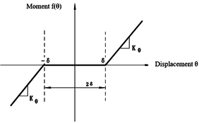
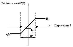
| − | Note that when <math>\boldsymbol{\tilde{f}}</math> is changed, the modal matrices used by each substructure are not affected and <math>\boldsymbol{Q}</math> is not necessary to be recalculated, simplifying the process of solving nonlinear equations. In Eq.(21), the nonlinear constraint contained in <math>\boldsymbol{\tilde{f}}</math> is the nonlinear function of the generalized displacement at the hinge connection, i.e. the elastic connection. In existing research, the treatment method for nonlinear free-play problems is generally to express nonlinear forces in segmented form and introduce them into dynamic equations for solution. Assuming <math>\theta </math> is a generalized displacement at the hinge, the free-play nonlinearity is modeled using the model in | + | Note that when <math>\boldsymbol{\tilde{f}}</math> is changed, the modal matrices used by each substructure are not affected and <math>\boldsymbol{Q}</math> is not necessary to be recalculated, simplifying the process of solving nonlinear equations. In Eq.(21), the nonlinear constraint contained in <math>\boldsymbol{\tilde{f}}</math> is the nonlinear function of the generalized displacement at the hinge connection, i.e. the elastic connection. In existing research, the treatment method for nonlinear free-play problems is generally to express nonlinear forces in segmented form and introduce them into dynamic equations for solution. Assuming <math>\theta </math> is a generalized displacement at the hinge, the free-play nonlinearity is modeled using the model in Bae et al. [26], and its moment is shown in [[#img-4|Figure 4]]. Meanwhile, friction is inevitable at the hinge connection, and that friction can serve as a stability factor is demonstrated in Sinha and Griffin [27]. Therefore, in order to weaken the various nonlinear motions of folding wings under free-play conditions, friction moment is used to weaken the influence of free-play nonlinearity. |
| − | <div class=" | + | <div id='img-1'></div> |
| − | + | {| class="wikitable" style="margin: 0em auto 0.1em auto;border-collapse: collapse;width:auto;" | |
| − | {| | + | |-style="background:white;" |
| + | |align="center" | | ||
| + | {|style="margin: 0em auto 0.1em auto;width:auto;" | ||
| + | |+ | ||
| + | |- | ||
| + | |style="text-align: center;padding:10px;"| [[Image:Review_423043765546-image110.png|282px]] | ||
| + | |style="text-align: center;padding:10px;"| [[Image:Review_423043765546-image111.png|center|246px]] | ||
|- | |- | ||
| − | | | + | |style="text-align: center;font-size: 75%;padding-bottom:10px;"|(a) Free-play nonlinearity [26] |
| − | | | + | |style="text-align: center;font-size: 75%;padding-bottom:10px;"|(b) Friction nonlinearity [27] |
| + | |} | ||
| + | |- | ||
| + | | style="background:#efefef;text-align:left;padding:10px;font-size: 85%;"| '''Figure 4'''. Structural nonlinear diagram | ||
|} | |} | ||
| − | |||
| − | |||
| − | |||
| − | |||
| − | |||
| − | |||
The expression for free-play nonlinearity is: | The expression for free-play nonlinearity is: | ||
| − | + | {| class="formulaSCP" style="width: 100%; text-align: left;" | |
| − | + | |- | |
| + | | | ||
| + | {| style="text-align: center; margin:auto;width: 100%;" | ||
| + | |- | ||
| + | | style="text-align: center;" | <math> f(\theta )=\left\{ \begin{array}{c} | ||
K_{\theta }(\theta -\delta ),(\theta >\delta )\\ | K_{\theta }(\theta -\delta ),(\theta >\delta )\\ | ||
0,\left(-\delta \leq \theta \leq \delta \right)\\ | 0,\left(-\delta \leq \theta \leq \delta \right)\\ | ||
K_{\theta }(\theta +\delta ),(\theta <-\delta ) | K_{\theta }(\theta +\delta ),(\theta <-\delta ) | ||
| − | \end{array}</math> | + | \end{array} \right.</math> |
| + | |} | ||
| + | | style="width: 5px;text-align: right;white-space: nowrap;" |(22) | ||
| + | |} | ||
| − | where, <math>\delta </math> is the free-play. When <math>\delta =0</math> , the moment is the linear function of <math>\theta </math> . | + | where, <math>\delta </math> is the free-play. When <math>\delta =0</math>, the moment is the linear function of <math>\theta </math>. |
The expression for frictional nonlinearity is: | The expression for frictional nonlinearity is: | ||
| − | + | {| class="formulaSCP" style="width: 100%; text-align: left;" | |
| − | + | |- | |
| + | | | ||
| + | {| style="text-align: center; margin:auto;width: 100%;" | ||
| + | |- | ||
| + | | style="text-align: center;" | <math> f{}'(\theta )=\left\{ \begin{array}{c} | ||
f_0,(\theta >\delta {}')\\ | f_0,(\theta >\delta {}')\\ | ||
K_{\theta '}\theta ,(-\delta {}'\leq \theta \leq \delta {}')\\ | K_{\theta '}\theta ,(-\delta {}'\leq \theta \leq \delta {}')\\ | ||
-f_0,(\theta <-\delta {}') | -f_0,(\theta <-\delta {}') | ||
| − | \end{array}</math> | + | \end{array}\right. </math> |
| + | |} | ||
| + | | style="width: 5px;text-align: right;white-space: nowrap;" |(23) | ||
| + | |} | ||
| − | |||
| − | + | The non-linear characteristic of this friction is that when <math>\delta {}'</math> is small, the friction moment <math>f{}'(\theta )</math> is equal to the product of the friction stiffness and the deflection angle <math>\theta </math>. When the moment is greater than <math>f_0</math>, the friction stiffness <math>K_{\theta '}</math> is 0, and the friction moment remains constant. Introducing frictional nonlinearity with respect to four independent nonlinear degrees of freedom into the nonlinear aeroelastic motion equation of free-play can achieve the analysis of free-play and frictional nonlinear aeroelastic response. | |
| − | < | + | Here, introducing aerodynamic state variables <math>\boldsymbol{q}_a</math>, the minimum state method is used to approximate the rational function of frequency domain aerodynamics, the state space form of the aeroelastic equation is: |
| − | + | ||
| + | {| class="formulaSCP" style="width: 100%; text-align: left;" | ||
| + | |- | ||
| + | | | ||
| + | {| style="text-align: center; margin:auto;width: 100%;" | ||
| + | |- | ||
| + | | style="text-align: center;" | <math>\left\{\begin{array}{c} | ||
\boldsymbol{\dot{q}}\\ | \boldsymbol{\dot{q}}\\ | ||
\boldsymbol{\ddot{q}}\\ | \boldsymbol{\ddot{q}}\\ | ||
| Line 326: | Line 548: | ||
\boldsymbol{\tilde{f}}\\ | \boldsymbol{\tilde{f}}\\ | ||
\boldsymbol{0} | \boldsymbol{0} | ||
| − | \end{array}\right\}</math> | + | \end{array}\right\} </math> |
| + | |} | ||
| + | | style="width: 5px;text-align: right;white-space: nowrap;" |(24) | ||
| + | |} | ||
| − | where, <math>\boldsymbol{\overline{M}}=\boldsymbol{\tilde{M}}-q_d{\left(b/V\right)}^2\boldsymbol{S}^T\boldsymbol{A}_\mbox{2}\boldsymbol{S}</math> , <math>\boldsymbol{\overline{D}}=-q_d\left(b/V\right)\boldsymbol{S}^T\boldsymbol{A}_\mbox{1}\boldsymbol{S}</math> , <math>\boldsymbol{\overline{K}}=\boldsymbol{\tilde{K}}-q_d\boldsymbol{S}^T\boldsymbol{A}_0\boldsymbol{S}</math> . <math>\boldsymbol{A}_0</math> , <math>\boldsymbol{A}_\mbox{1}</math> , <math>\boldsymbol{A}_\mbox{2}</math> , <math>\boldsymbol{D}_s</math> and <math>\boldsymbol{E}_s</math> , which are all unknown matrices in the minimum state approximation. <math>\boldsymbol{R}_s</math> is the aerodynamic lag matrix, and <math>b</math> is the reference length. | + | where, <math>\boldsymbol{\overline{M}}=\boldsymbol{\tilde{M}}-q_d{\left(b/V\right)}^2\boldsymbol{S}^T\boldsymbol{A}_\mbox{2}\boldsymbol{S}</math>, <math>\boldsymbol{\overline{D}}=-q_d\left(b/V\right)\boldsymbol{S}^T\boldsymbol{A}_\mbox{1}\boldsymbol{S}</math>, <math>\boldsymbol{\overline{K}}=\boldsymbol{\tilde{K}}-q_d\boldsymbol{S}^T\boldsymbol{A}_0\boldsymbol{S}</math>. <math>\boldsymbol{A}_0</math>, <math>\boldsymbol{A}_\mbox{1}</math>, <math>\boldsymbol{A}_\mbox{2}</math>, <math>\boldsymbol{D}_s</math> and <math>\boldsymbol{E}_s</math>, which are all unknown matrices in the minimum state approximation. <math>\boldsymbol{R}_s</math> is the aerodynamic lag matrix, and <math>b</math> is the reference length. |
| − | == | + | ==4. Analysis and discussion== |
Only the nonlinear aeroelastic response of the folding wing in the fully unfolded state has been analyzed here. The mass matrix and stiffness matrix of each substructure of the folding wing are obtained through DMAP language. The modified Doublet Lattice Method is used to obtain the unsteady aerodynamic forces of a folding wing in the frequency domain, and the expression of the aeroelastic equation in the state space is obtained through the minimum state approximation. For each substructure, six vibration modes are retained, and 10 degrees of freedom are coupled to each other through MPC and torsion springs at the interface, while 2 independent nonlinear degrees of freedom are retained. The final dynamic equation of the folding wing obtained is 22. After introducing 4 aerodynamic state variables, the aeroelastic equation in the state space is finally obtained, that is, Eq.(24) is 48, Finally, the time-domain aeroelastic response of the folding wing is obtained using the Runge-Kutta method in MATLAB. | Only the nonlinear aeroelastic response of the folding wing in the fully unfolded state has been analyzed here. The mass matrix and stiffness matrix of each substructure of the folding wing are obtained through DMAP language. The modified Doublet Lattice Method is used to obtain the unsteady aerodynamic forces of a folding wing in the frequency domain, and the expression of the aeroelastic equation in the state space is obtained through the minimum state approximation. For each substructure, six vibration modes are retained, and 10 degrees of freedom are coupled to each other through MPC and torsion springs at the interface, while 2 independent nonlinear degrees of freedom are retained. The final dynamic equation of the folding wing obtained is 22. After introducing 4 aerodynamic state variables, the aeroelastic equation in the state space is finally obtained, that is, Eq.(24) is 48, Finally, the time-domain aeroelastic response of the folding wing is obtained using the Runge-Kutta method in MATLAB. | ||
| − | + | ===4.1 Aerodynamic model validation=== | |
To verify the correctness of the modified Doublet Lattice Method, two examples are presented here. | To verify the correctness of the modified Doublet Lattice Method, two examples are presented here. | ||
| − | Example 1: In | + | '''Example 1''': In Qian [29], an example is given to calculate the lift and lift coefficient of a swept wing. Its aspect ratio is 5 and the taper ratio is 1, as shown in [[#img-5|Figure 5]]. Take its aspect as 5, root chord as 1, leading edge sweep angle as <math>{45}^{\circ }</math>, Mach number <math>M_{\infty }=0.2</math>, <math>\alpha =1^{\boldsymbol{\mbox{°}}}</math>. When the frequency is zero, the modified Doublet Lattice Method will degenerate into the vortex lattice method, which is the steady part of the modified Doublet Lattice Method. The lift and lift coefficient of the swept wing are obtained using the steady part, and the comparison results are shown in [[#tab-1|Table 1]]. |
| − | <div class=" | + | <div id='img-5'></div> |
| − | + | {| class="wikitable" style="margin: 0em auto 0.1em auto;border-collapse: collapse;width:auto;" | |
| + | |-style="background:white;" | ||
| + | |style="text-align: center;padding:10px;"| [[Image:Review_423043765546-image137.png|450px]] | ||
| + | |- | ||
| + | | style="background:#efefef;text-align:left;padding:10px;font-size: 85%;"| '''Figure 5'''. Wing geometry dimensions | ||
| + | |} | ||
| − | |||
| − | |||
| − | <div class="center" style=" | + | <div class="center" style="font-size: 85%;">'''Table 1'''. Comparison results</div> |
| − | Table 1 Comparison | + | |
| − | {| style=" | + | <div id='tab-1'></div> |
| + | {| class="wikitable" style="margin: 1em auto 0.1em auto;border-collapse: collapse;font-size:85%;width:auto;" | ||
| + | |-style="text-align:center" | ||
| + | ! !! Qian [29] !! Present !! Relative error (%) | ||
|- | |- | ||
| − | | style=" | + | | style="text-align: center;vertical-align: top;"|Lift ( <math>N</math> ) |
| − | | style=" | + | | style="text-align: center;vertical-align: top;"|848.554 |
| − | | style=" | + | | style="text-align: center;vertical-align: top;"|851.296 |
| − | | style=" | + | | style="text-align: center;vertical-align: top;"|0.323 |
|- | |- | ||
| − | | style=" | + | | style="text-align: center;vertical-align: top;"|Lift Coefficient |
| − | + | | style="text-align: center;vertical-align: top;"|0.059921 | |
| − | + | | style="text-align: center;vertical-align: top;"|0.0601131 | |
| − | + | | style="text-align: center;vertical-align: top;"|0.321 | |
| − | + | ||
| − | + | ||
| − | | style=" | + | |
| − | | style=" | + | |
| − | | style=" | + | |
|} | |} | ||
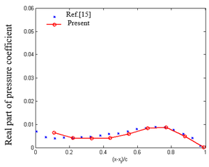
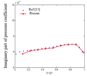
| − | Example 2: In | + | '''Example 2''': In Zhao [15], a swept wing with equal chord length, leading edge sweep angle <math>\Lambda ={25}^{\boldsymbol{\mbox{°}}}</math>, half span length <math>l=3.0</math>, aspect ratio <math>AR=3.0</math>, as shown in [[#img-6|Figure 6]]. There is a control surface at 50% of the half span length, with the chord length of the control surface being <math>1/3</math> of the chord length c of the wing, and the amplitude of the control surface oscillates harmoniously. Reduced frequency <math>k=0.372</math>, Mach number <math>M_{\infty }=0</math>. Using the correction method, the changes in the real and imaginary parts of the pressure coefficients of the chord distribution units with a half span length of 42.5% and a half span length of 72.5% are shown in [[#img-7|Figure 7]]. |
| − | <div | + | <div id='img-6'></div> |
| − | + | {| class="wikitable" style="margin: 0em auto 0.1em auto;border-collapse: collapse;width:auto;" | |
| − | + | |-style="background:white;" | |
| − | + | |style="text-align: center;padding:10px;"| [[Image:Review_423043765546-image145.png|444px]] | |
| − | + | ||
| − | + | ||
| − | + | ||
| − | + | ||
| − | + | ||
|- | |- | ||
| − | | | + | | style="background:#efefef;text-align:left;padding:10px;font-size: 85%;"| '''Figure 6'''. Swept wing with equal chord length |
| − | + | ||
|} | |} | ||
| − | |||
| − | |||
| − | |||
| − | {| | + | <div id='img-7'></div> |
| − | [[Image: | + | {| class="wikitable" style="margin: 0em auto 0.1em auto;border-collapse: collapse;width:auto;" |
| − | [[Image: | + | |-style="background:white;" |
| + | |align="center" | | ||
| + | {|style="margin: 0em auto 0.1em auto;width:auto;" | ||
| + | |+ | ||
| + | |- | ||
| + | |style="text-align: center;padding:10px;"| [[Image:Review_423043765546-image146.png|300px]] | ||
| + | |style="text-align: center;padding:10px;"| [[Image:Review_423043765546-image147.png|center|290px]] | ||
| + | |- | ||
| + | | colspan="2" style="text-align: center;font-size: 75%;padding-bottom:10px;"|(a) Chordal distribution of pressure coefficient (at 42.5% of half span) | ||
| + | |- | ||
| + | |style="text-align: center;padding:10px;"| [[Image:Review_423043765546-image148.png|298px]] | ||
| + | |style="text-align: center;padding:10px;"| [[Image:Review_423043765546-image149.png|center|350px]] | ||
| + | |- | ||
| + | | colspan="2" style="text-align: center;font-size: 75%;padding-bottom:10px;"|(b) Chordal distribution of pressure coefficient (at 72.5% of half span) | ||
| + | |} | ||
| + | |- | ||
| + | | style="background:#efefef;text-align:left;padding:10px;font-size: 85%;"| '''Figure 7'''. Chordal distribution of pressure coefficient | ||
|} | |} | ||
| − | |||
| − | |||
| − | |||
| − | |||
| − | |||
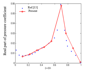
| − | In Example 1, four elements are used for both the left and right wings. The modified Doublet Lattice Method is reduced to zero frequency and degenerated into the vortex lattice method, which uses the steady part of the modified Doublet Lattice Method to obtain lift and lift coefficients. The relative error is within an acceptable range. In Example 2, the trend of the results obtained using the modified Doublet Lattice Method is basically similar to the trend of the results in | + | In Example 1, four elements are used for both the left and right wings. The modified Doublet Lattice Method is reduced to zero frequency and degenerated into the vortex lattice method, which uses the steady part of the modified Doublet Lattice Method to obtain lift and lift coefficients. The relative error is within an acceptable range. In Example 2, the trend of the results obtained using the modified Doublet Lattice Method is basically similar to the trend of the results in Zhao [15]. Due to the sparsity of the element, the obtained curve is not smooth enough. By further increasing the number of elements in the chord and spanwise directions, this result can be improved. Comparing the chordal distribution of pressure coefficients at different spans, it can be seen that compared to the pressure coefficient distribution at 42.5% half span, the distribution at 72.5% half span has a significant change, mainly due to the deflection angle of the control surface, making the pressure coefficient distribution at the trailing edge more prominent. From the above two examples, it can be seen that the modified Doublet Lattice Method is correct. |
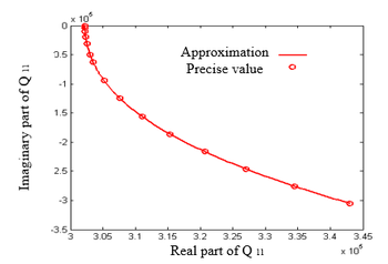
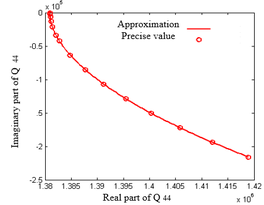
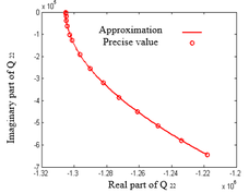
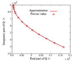
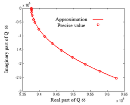
| − | Based on the modified Doublet Lattice Method, frequency domain unsteady aerodynamic calculations on folding wings is performed. Furthermore, the minimum state approximation method is used to fit the unsteady aerodynamic forces. The discrete form of the generalized aerodynamic force obtained in the frequency domain is given a lag matrix <math>\boldsymbol{R}_s</math> in advance. The real and imaginary parts of the generalized aerodynamic force matrix at 15 reduced frequency points are fitted. And <math>\boldsymbol{B}_d</math> , <math>\boldsymbol{Q}_d</math> , <math>\boldsymbol{B}_e</math> , <math>\boldsymbol{Q}_e</math> are known, and then the steady-state aerodynamic force data is used to form constraint conditions for iteration. Here are some fitting results, as shown in | + | Based on the modified Doublet Lattice Method, frequency domain unsteady aerodynamic calculations on folding wings is performed. Furthermore, the minimum state approximation method is used to fit the unsteady aerodynamic forces. The discrete form of the generalized aerodynamic force obtained in the frequency domain is given a lag matrix <math>\boldsymbol{R}_s</math> in advance. The real and imaginary parts of the generalized aerodynamic force matrix at 15 reduced frequency points are fitted. And <math>\boldsymbol{B}_d</math>, <math>\boldsymbol{Q}_d</math>, <math>\boldsymbol{B}_e</math>, <math>\boldsymbol{Q}_e</math> are known, and then the steady-state aerodynamic force data is used to form constraint conditions for iteration. Here are some fitting results, as shown in [[#img-8|Figure 8]]. It can be seen that the approximate value matches the exact value well, and after obtaining the unknown matrix in the minimum state approximation, time-domain aeroelastic analysis can be achieved. |
| − | <div id= | + | <div id='img-8'></div> |
| − | + | {| class="wikitable" style="margin: 0em auto 0.1em auto;border-collapse: collapse;width:auto;" | |
| − | {| | + | |-style="background:white;" |
| + | |align="center" | | ||
| + | {|style="margin: 0em auto 0.1em auto;width:auto;" | ||
| + | |+ | ||
|- | |- | ||
| − | | [[Image: | + | |style="text-align: center;padding:10px;"| [[Image:Review_423043765546-image155.png|264px]] |
| − | | [[Image: | + | |style="text-align: center;padding:10px;"| [[Image:Review_423043765546-image156.png|center|228px]] |
| + | |- | ||
| + | |style="text-align: center;font-size: 75%;padding-bottom:10px;"|(a) <math>\boldsymbol{Q}_{11}</math> | ||
| + | |style="text-align: center;font-size: 75%;padding-bottom:10px;"|(b) <math>\boldsymbol{Q}_{22}</math> | ||
| + | |- | ||
| + | |style="text-align: center;padding:10px;"| [[Image:Review_423043765546-image159.png|264px]] | ||
| + | |style="text-align: center;padding:10px;"| [[Image:Review_423043765546-image160.png|center|258px]] | ||
| + | |- | ||
| + | |style="text-align: center;font-size: 75%;padding-bottom:10px;"|(c) <math>\boldsymbol{Q}_{33}</math> | ||
| + | |style="text-align: center;font-size: 75%;padding-bottom:10px;"|(d) <math>\boldsymbol{Q}_{44}</math> | ||
| + | |- | ||
| + | |style="text-align: center;padding:10px;"| [[Image:Review_423043765546-image163.png|252px]] | ||
| + | |style="text-align: center;padding:10px;"| [[Image:Review_423043765546-image164.png|center|258px]] | ||
| + | |- | ||
| + | |style="text-align: center;font-size: 75%;padding-bottom:10px;"|(e) <math>\boldsymbol{Q}_{55}</math> | ||
| + | |style="text-align: center;font-size: 75%;padding-bottom:10px;"|(f) <math>\boldsymbol{Q}_{66}</math> | ||
|} | |} | ||
| − | |||
| − | |||
| − | |||
| − | |||
| − | |||
| − | |||
| − | |||
|- | |- | ||
| − | | | + | | style="background:#efefef;text-align:left;padding:10px;font-size: 85%;"| '''Figure 8'''. Minimum state approximation results for unsteady aerodynamics of folding wings |
| − | + | ||
|} | |} | ||
| − | |||
| − | + | ===4.2 Structural nonlinear aeroelastic analysis=== | |
| + | According to Li et al. [21], it can be seen that when <math>\delta =0</math> , the model is equal to the linear model. And the linear flutter velocity <math>V_f=31.25m/s</math> . The <math>\delta =0.02\mbox{°}</math>, <math>\delta =0.2\mbox{°}</math>, <math>\delta =1\mbox{°}</math> of the inner and outer hinges are taken as examples. An initial disturbance of 0.01mm is added to the normal direction of the trailing edge node of the wing tip to obtain the velocity at which the normal displacement response of the leading edge of the folding wing tip begins to diverge. Assuming <math>K_{\theta '}=1Nm/rad</math>, the different moments are introduced separately, the displacement response obtained are shown in [[#img-9|Figures 9]] and [[#img-10|10]]. | ||
| − | {| | + | <div id='img-9'></div> |
| + | {| class="wikitable" style="margin: 0em auto 0.1em auto;border-collapse: collapse;width:auto;" | ||
| + | |-style="background:white;" | ||
| + | |align="center" | | ||
| + | {|style="margin: 0em auto 0.1em auto;width:auto;" | ||
| + | |+ | ||
|- | |- | ||
| − | | [[Image: | + | |style="text-align: center;padding:10px;"| [[Image:Review_423043765546-image173.png|326px]] |
| − | | [[Image: | + | |style="text-align: center;padding:10px;"| [[Image:Review_423043765546-image174.png|center|302px]] |
| + | |- | ||
| + | |style="text-align: center;font-size: 75%;padding-bottom:10px;"| (a) <math>V=1.01V_f</math>, <math>\delta =0.02\mbox{°}</math>, <math>f_0=0.005Nm</math> | ||
| + | |style="text-align: center;font-size: 75%;padding-bottom:10px;"|(b) <math>V=0.99V_f</math>, <math>\delta =0.2\mbox{°}</math>, <math>f_0=0.02Nm</math> | ||
| + | |- | ||
| + | |colspan="2" style="text-align: center;padding:10px;"| [[Image:Review_423043765546-image181.png|348px]] | ||
| + | |- | ||
| + | |colspan="2" style="text-align: center;font-size: 75%;padding-bottom:10px;"|(c) <math>V=0.96V_f</math>, <math>\delta =1\mbox{°}</math>, <math>f_0=0.05Nm</math> | ||
|} | |} | ||
| − | |||
| − | |||
| − | |||
| − | |||
| − | |||
| − | |||
| − | |||
| − | |||
| − | |||
| − | |||
| − | |||
| − | |||
| − | |||
| − | |||
|- | |- | ||
| − | | | + | | style="background:#efefef;text-align:left;padding:10px;font-size: 85%;"| '''Figure 9'''. Friction at the inner hinge |
| − | + | ||
|} | |} | ||
| − | |||
| − | |||
| − | |||
| − | |||
| − | |||
| − | |||
| − | <div class=" | + | <div id='img-10'></div> |
| − | ( | + | {| class="wikitable" style="margin: 0em auto 0.1em auto;border-collapse: collapse;width:auto;" |
| − | + | |-style="background:white;" | |
| − | + | |align="center" | | |
| − | + | {|style="margin: 0em auto 0.1em auto;width:auto;" | |
| − | + | |+ | |
| − | + | |- | |
| − | + | |style="text-align: center;padding:10px;"| [[Image:Review_423043765546-image185.png|352px]] | |
| − | + | |style="text-align: center;padding:10px;"| [[Image:Review_423043765546-image186.png|center|352px]] | |
| + | |- | ||
| + | |style="text-align: center;font-size: 75%;padding-bottom:10px;"| (a) <math>V=1.0V_f</math>, <math>\delta =0.02\mbox{°}</math>, <math>f_0=0.007Nm</math> | ||
| + | |style="text-align: center;font-size: 75%;padding-bottom:10px;"|(b) <math>V=0.97V_f</math>, <math>\delta =0.2\mbox{°}</math>, <math>f_0=0.01Nm</math> | ||
| + | |- | ||
| + | |colspan="2" style="text-align: center;padding:10px;"| [[Image:Review_423043765546-image193.png|332px]] | ||
|- | |- | ||
| − | | | + | |colspan="2" style="text-align: center;font-size: 75%;padding-bottom:10px;"|(c) <math>V=0.95V_f</math>, <math>\delta =1\mbox{°}</math>, <math>f_0=0.05Nm</math> |
| − | | | + | |} |
| + | |- | ||
| + | | style="background:#efefef;text-align:left;padding:10px;font-size: 85%;"| '''Figure 10'''. Friction at the outer hinge | ||
|} | |} | ||
| − | |||
| − | |||
| − | |||
| − | + | From [[#img-9|Figures 9]] and [[#img-10|10]], it can be seen that when the friction stiffness is constant, an appropriate friction moment can suppress the divergence of displacement. Friction nonlinearity can effectively weaken the divergent motion of the normal displacement of the leading edge node of the wing tip, transforming it from an unstable motion tending towards divergence to a limit cycle motion with limited amplitude. It can be observed that the normal displacement response of the wingtip is centered around the zero position. This is because both free-play nonlinearity and friction nonlinearity are centrally symmetric, and after superposition, they remain centrally symmetric. This result also verifies the correctness of the model proposed in this paper. | |
| − | [[ | + | |
| − | + | In order to further clarify the influence of physical parameters of friction nonlinearity on the nonlinear aeroelasticity of free-play, the effects of moment <math>f_0</math> and frictional stiffness <math>K_{\theta '}</math> on the response of free-play nonlinear aeroelastic systems are analyzed. Taking the free-play <math>\delta =1\mbox{°}</math> between the inner and outer hinges as an example, the displacement tends to diverge at a speed of <math>V=0.96V_f</math> and <math>V=0.95V_f</math>, the effect of frictional nonlinearity on the aeroelasticity of the free-play is shown in [[#img-11|Figure 11]]. | |
| − | + | ||
| − | <div class=" | + | <div id='img-11'></div> |
| − | + | {| class="wikitable" style="margin: 0em auto 0.1em auto;border-collapse: collapse;width:auto;" | |
| − | + | |-style="background:white;" | |
| − | + | |align="center" | | |
| − | + | {|style="margin: 0em auto 0.1em auto;width:auto;" | |
| − | + | |+ | |
| − | + | |- | |
| − | + | |style="text-align: center;padding:10px;"| [[Image:Review_423043765546-image199.png|302px]] | |
| − | + | |style="text-align: center;padding:10px;"| [[Image:Review_423043765546-image200.png|center|332px]] | |
| − | + | ||
|- | |- | ||
| − | | | + | |style="text-align: center;font-size: 75%;padding-bottom:10px;"|(a) Influence of initial moment |
| − | | | + | |style="text-align: center;font-size: 75%;padding-bottom:10px;"|(b) Influence of friction stiffness |
| + | |} | ||
| + | |- | ||
| + | | style="background:#efefef;text-align:left;padding:10px;font-size: 85%;"| '''Figure 11'''. Influence of nonlinear friction on free-play aeroelasticity | ||
|} | |} | ||
| − | |||
| − | |||
| − | |||
| − | + | From [[#img-11|Figure 11]], it can be seen that as the initial moment <math>f_0</math> increases, the amplitude of the wingtip normal displacement decreases. As the friction stiffness <math>K_{\theta '}</math> increases, the amplitude of normal displacement at the leading edge of the wing tip does not change significantly. In [[#img-11|Figure 11]](a), <math>K_{\theta '}=1Nm/rad</math>, as the initial moment <math>f_0</math> increases, <math>\delta {}'</math> increases. When <math>\delta {}'</math> reaches a certain degree, the effect of the initial moment and the external moment caused by free-play nonlinearity is opposite, weakening the free-play nonlinearity. In [[#img-11|Figure 11]](b), <math>f_0=0.05Nm</math>, as the friction stiffness <math>K_{\theta '}</math> increases, <math>\delta {}'</math> decreases. In a smaller displacement range, <math>K_{\theta '}\theta </math> plays a major role, so the initial moment <math>f_0</math> still plays a major role in a larger displacement range. This phenomenon indicates that compared to frictional stiffness, frictional moment plays an important role in reducing response amplitude. At the same time, when friction nonlinearity is added to the free-play nonlinearity at the outer hinge, the normal amplitude of the wing tip is always larger than when friction nonlinearity is added to the free-play nonlinearity at the inner hinge. In summary, to a certain extent, frictional nonlinearity can effectively reduce vibration amplitude, which is beneficial nonlinearity. | |
| − | + | ||
| − | + | ||
| − | + | ||
| − | == | + | ==5. Conclusions== |
The structural nonlinear aeroelastic analysis of folding wings is conducted by the modified Doublet Lattice Method. Firstly, a modified Doublet Lattice Method is studied to relax the aspect ratio limitation of aerodynamic elements, and its correctness is verified through numerical examples. Secondly, the rational function approximation method is discussed, and the modified Doublet Lattice Method is approximated using the minimum state method to obtain the unsteady aerodynamic forces in the time domain. Finally, the aeroelastic characteristics of a folding wing with free-play and friction nonlinearities are studied by combining time-domain unsteady aerodynamics and nonlinear structural dynamics models. The following conclusions can be drawn: | The structural nonlinear aeroelastic analysis of folding wings is conducted by the modified Doublet Lattice Method. Firstly, a modified Doublet Lattice Method is studied to relax the aspect ratio limitation of aerodynamic elements, and its correctness is verified through numerical examples. Secondly, the rational function approximation method is discussed, and the modified Doublet Lattice Method is approximated using the minimum state method to obtain the unsteady aerodynamic forces in the time domain. Finally, the aeroelastic characteristics of a folding wing with free-play and friction nonlinearities are studied by combining time-domain unsteady aerodynamics and nonlinear structural dynamics models. The following conclusions can be drawn: | ||
| Line 515: | Line 741: | ||
(3) Friction moment plays an important role in reducing response amplitude and is a beneficial nonlinearity. | (3) Friction moment plays an important role in reducing response amplitude and is a beneficial nonlinearity. | ||
| − | |||
| − | + | '''Funding:''' This research is supported by Natural Science Basic Research Plan in Shaanxi Province of China (2021JQ-847 and 2023-JC-YB-076). | |
| + | |||
| + | ==References== | ||
| + | <div class="auto" style="text-align: left;width: auto; margin-left: auto; margin-right: auto;font-size: 85%;"> | ||
| − | [1] Chen S S, Jia M L, Liu Y X,et al. Development status on deformation modes and key | + | [1] Chen S.S., Jia M.L., Liu Y.X., et al. Development status on deformation modes and key technologies of aerodynamic layout design about morphing aircraft (in Chinese). Acta Aeronautica et Astronautica Sinica, 45(5), 629595, 2024. |
| − | [2] Ma | + | [2] Ma H., Song B.F., Zhou Z.B., Zhang D.S.H.Analysis of the development status of multi-section morphing wing technology (in Chinese).Tactical Missile Technology, 2024. [https://doi.org/10.16358/j.issn.1009-1300.20230121 https://doi.org/10.16358/j.issn.1009-1300.20230121, 2024-02-08]. |
| − | [3] Snyder M | + | [3] Snyder M.P., Sanders B., Eastep F.E., Frank G.J. Vibration and flutter characteristics of a folding wing. Journal of Aircraft, 46(3):791-799, 2009. |
| − | [4]Wang | + | [4] Wang I., Gibbs S.C., Dowell E.H. Aeroelastic model of multisegmented folding wings:Theory and experiment. Journal of Aircraft, 49(3)911-921, 2012. |
| − | [5] Lee D | + | [5] Lee D.H., Weisshaar T.A. Aeroelastic studies on a folding wing configuration. 46th AIAA/ ASME/ASCE/AHS/ASC Structures, Structural Dynamics and Materials Conference, Austin, Texas, 2005. |
| − | [6] Lee D | + | [6] Lee D.H., Chen P.C. Nonlinear aeroelastic studies on a folding wing configuration with free play hinge nonlinearity. 47th AIAA/ASME/ASCE/AHS/ASCStructures, Structural Dynamics and Materials Conference, Newport, Rhode Island, 2006. |
| − | [7] Attar | + | [7] Attar P., Tang D., Dowell E.H. Nonlinear aeroelastic study for folding wing structures. AIAA Journal, 48(10)2187-2195, 2010. |
| − | [8] Reich G | + | [8] Reich G.W., Bowman J.C., Sanders B., et al. Development of an integrated aeroelastic multibody morphing simulation tool. 47th AIAA/ASME/ASCE/AHS/ASC Structures, Structural Dynamics and Materials Conference, Newport, Rhode Island, 2006. |
| − | [9] Zhao Y. H., Hu H.Y | + | [9] Zhao Y.H., Hu H.Y. Parameterized aeroelastic modeling and flutter analysis for a folding wing. Journal of Sound Vibration, 331:208-324, 2012. |
| − | [10] Tang D., Dowell E. H | + | [10] Tang D., Dowell E.H. Theoretical and experimental aeroelastic study for folding wing structures. Journal of Aircraft, 45(4):1136-1147, 2008. |
| − | [11] Hu | + | [11] Hu W., Yang Z., Gu Y., Wang X. The nonlinear aeroleastic characteristics of a folding wing with cubic stiffness. Journal of Sound and Vibration, 400:22-39, 2017. |
| − | [12] Ni Y.G., Zhang W., Lv Y | + | [12] Ni Y.G., Zhang W., Lv Y. Fast structural dynamic modeling and analysis for horizontally folding wing. Revista Internacional de Métodos Numéricos para Cálculo y Diseño en Ingeniería, 37(3), 35, 2021. |
| − | [13] Ni Y.G., Zhang W., Lv Y.. Multi-body dynamics modeling and transient characteristics analysis for a folding wing | + | [13] Ni Y.G., Zhang W., Lv Y.. Multi-body dynamics modeling and transient characteristics analysis for a folding wing. Revista Internacional de Métodos Numéricos para Cálculo y Diseño en Ingeniería, 37(1), 4, 2021. |
| − | [14] Yang N, Wu Zh. G., Yang Ch., Cao Q.K | + | [14] Yang N., Wu Zh.G., Yang Ch., Cao Q.K. Flutter analysis of a folding wing with structural nonlinearity. Engineeing Mechanics, 29(2):197-204, 2012. |
| − | [15] Zhao Y | + | [15] Zhao Y.H. Aeroelasticity and control. Science Press, Beijing, 2007. |
| − | [16] Verstraete M. L., Preidikman S., | + | [16] Verstraete M.L., Preidikman S., Roccia B.A., Mook D.T. A numerical nodel to study the nonlinear and unsteady aerodynamics of bioinspired morphing-wing comcepts. International Journal of Micro Air Vehicles, 7(3):327-345, 2015. |
| − | [17] Albano E., Rodden W. P | + | [17] Albano E., Rodden W.P. A doublet-lattice method for calculating lift distributions on oscillating surfaces in subsonic flows. AIAA Journal, 7(2):279-285, 1969. |
| − | [18] Landabl M. T | + | [18] Landabl M.T. Kernel function for nonplanar oscillating surfaces in a subsonic flow. AIAA Journal, 5(5):1045-1046, 1967. |
| − | [19] Rodden W. P., Giesing J. P., Kalman T. P | + | [19] Rodden W.P., Giesing J.P., Kalman T.P. Refinement of the nonplanar aspects of the subsonic doublet-lattice lifting surface method. Journal of Aircraft, 9(1):69-73, 1972. |
| − | [20] Rodden W. P., Taylor P. F., Mcintosh S. C | + | [20] Rodden W.P., Taylor P.F., Mcintosh S.C. Further refinement of the subsonic doublet-dattice method. Journal of Aircraft, 35(5):720-727, 1998. |
| − | [21] Li P. CH., Ni Y.G., Hou Ch., Wan X. P., Zhao M. Y. Nonlinear aeroelastic aodeling of a folding wing structure | + | [21] Li P.CH., Ni Y.G., Hou Ch., Wan X.P., Zhao M.Y. Nonlinear aeroelastic aodeling of a folding wing structure. Journal of Physics: Conf. Series, 1215, 012009, 2019 |
| − | [22] Jones R. T | + | [22] Jones R.T. The unsteady lift of a wing of finite aspect ratio. NACA Report-681, 1941. |
| − | [23] Roger K. L | + | [23] Roger K.L. Airplane math modeling methods for active control design. AGARD-CP, 228:4.1-4.11, 1977. |
| − | [24] Karpel M | + | [24] Karpel M. Extensions to the minimum-state aeroelastic modeling method. AIAA Journal, 29(11):2007-2009, 1991. |
| − | [25] Vepa R | + | [25] Vepa R. Finite state modeling of aeroelastic systems. NASA CR-2779, 1977. |
| − | [26] Bae J.S., Inman D.J., Lee I | + | [26] Bae J.S., Inman D.J., Lee I. Effects of structural nonlinearity on subsonic aeroelastic characteristcs of an aircraft wing with control surface. Journal of Fluids and Structures, 19(6):747-763, 2004. |
| − | [27] Sinha A., Griffin J. H | + | [27] Sinha A., Griffin J.H. Effects of friction dampers on aerodynamically unstable rotor stages. AIAA Journal, 23(2):262-270, 1985. |
| − | [28] Liu B. H., Li M., Tan T. C | + | [28] Liu B.H., Li M., Tan T.C. Flutter study of a two-dimensional airfoil with structural nonlinearities. Engineering Mechanics, 30(4):448-454, 2013. |
| − | [29] Qian Y. J | + | [29] Qian Y.J. Aerodynamics. Beijing University of Aeronautics and Astronautics Press, Beijing, 2004. |
Latest revision as of 11:56, 12 July 2024
Abstract
The structural nonlinear aeroelastic analysis of folding wings is conducted by integrating the modified Doublet Lattice Method in this paper. Firstly, a modified Doublet Lattice Method is investigated to relax the aspect ratio limitation of aerodynamic elements, and its correctness is verified through numerical examples. Secondly, the rational function approximation method is discussed, and the modified Doublet Lattice Method is approximated using the minimum state method to obtain the unsteady aerodynamic forces in the time domain. Finally, the aeroelastic characteristics of a folding wing with free-play and friction nonlinearity are studied by integrating time-domain unsteady aerodynamics with the nonlinear structural dynamics model. The results show that the modified Doublet Lattice Method, which relaxes the aspect ratio limitation of aerodynamic grid elements, is feasible and effective; Friction can suppress the influence of free-play nonlinearity on aeroelastic response.
Keywords: Folding wing, modified doublet lattice method, rational function approximation, structural nonlinearity
1. Introduction
With the complexity of aircraft flight missions, the ability to adapt to multiple tasks and achieving “one aircraft with multiple capabilities” has gradually become a new requirement for aircraft design. As a result, morphing aircrafts that can change the shape of aircraft to adapt to different flight environments, improve aerodynamic performance, and expand flight envelopes have emerged, and have shown broad application prospects in the aviation field [1]. At present, the morphing mode that has been extensively studied is still folding wings [2].
Snyder et al. analyzed the vibration and flutter characteristics of the folding wing configuration [3]. Wang et al. conducted relevant research on the aeroelasticity and structural mechanics of folding wing models [4]. Lee et al. utilized MSC.NASTRAN and ZEARO software to analyze the relationship between flutter and folding angle [5], and further conducted structural nonlinear aeroelastic analysis [6]. Attar et al. conducted theoretical analysis and experimental verification on the nonlinear aeroelastic response of the folding wing structures [7]. Reich et al. analyzed and studied the aeroelastic issues during folding and unfolding processes [8]. Zhao et al. established a parameterized aeroelastic model of a folding wing using component synthesis method and Doublet Lattice Method, and compared the flutter boundary obtained from the parameterized model with the results obtained through MSC.NASTRAN [9]. Tang et al. established a linear aeroelastic equation for a folding wing structure using a three-dimensional time-domain vortex lattice method, and studied its stable boundary. Finally, the influence of different parameters on the flutter boundary was discussed and compared with the results of experiments [10]. Hu et al. established an aeroelastic model with cubic nonlinearity using the Lagrange equation and a surrogate model based on the Doublet Lattice Method, and conducted corresponding analysis [11]. Ni et al. used mode synthesis method and Doublet Lattice Method to analyze the flutter boundary of a folding wing, and further analyzed the aeroelastic response during the folding process using multi-body dynamics theory [12-13]. Yang et al. conducted nonlinear aeroelastic analysis in both frequency and time domains for folding wings with free-play, using mode synthesis and descriptive function methods [14].
In existing research, the calculation of aerodynamic forces is mostly based on the Doublet Lattice Method. However, the Doublet Lattice Method generally requires the aspect ratio of the elements to be less than 3. In this case, a dense spanwise element must be adopted to improve computational accuracy, greatly increasing computational time and storage space [15]. Therefore, it is necessary to modify the Doublet Lattice Method to reduce the number of aerodynamic elements, and thus reduce the calculation time of unsteady aerodynamics in the frequency domain. In the research on structural nonlinear aeroelasticity, the influence of free-play on wings has been studied through experimental and numerical methods, but all of these studies have not provided a good solution to weaken the influence of free-play nonlinearity. Therefore, for the study of aeroelasticity of folding wings, on the one hand, it is necessary to modify the Doublet Lattice Method to improve computational efficiency. On the other hand, it is necessary to propose reasonable solutions to suppress the nonlinearity based on predicting nonlinear aeroelastic phenomena.
The modified Doublet Lattice Method is used to conduct structural nonlinear aeroelastic analysis of folding wings. Firstly, the Doublet Lattice Method is modified to relax the aspect ratio limitation of aerodynamic elements, and its correctness is verified through numerical examples. Secondly, the modified Doublet Lattice Method is approximated by rational functions by the minimum state method to obtain the unsteady aerodynamic forces in the time domain. Finally, by combining time-domain unsteady aerodynamics and nonlinear structural dynamics models, the aeroelastic characteristics of folding wings with structural nonlinearity are studied, and friction nonlinearity is used to suppress free-play nonlinearity.
2. Modified Doublet Lattice Method
Two methods have been developed to calculate the subsonic unsteady aerodynamics [16]. The first type is to assume the load function of the lift surface and the undetermined coefficients are determined based on the integral equation and boundary conditions. The second type is the Doublet Lattice Method. The difference between the Doublet Lattice Method and the vortex lattice method is that not only is a horseshoe vortex placed on the quarter chord of each aerodynamic element, but also an acceleration potential doublet is placed to simulate the unsteady term caused by wing motion. Compared with the first type of calculation method, the Doublet Lattice Method does not require the selection of appropriate load distribution functions [17-18], and it has good applicability for complex lift surfaces, considering the mutual interference of multiple wing surfaces and wing body combinations. Therefore, in recent years, researchers have conducted a lot of research on the relevant improvement methods of Doublet Lattice Method [19-20].
The subsonic Doublet Lattice Method based on small perturbation linearized potential flow frequency domain equations is one of the methods for calculating unsteady aerodynamics. The basic principle is that when the aircraft wing undergoes harmonic vibration, an acceleration potential doublet can be distributed on the wing. According to the normal downwash amplitude generated on the wing, the corresponding vibration boundary conditions must be met, and the expression for pressure difference can be obtained. The relationship between the amplitude of the pressure difference and the amplitude of the normal downwash velocity on the lift surface can be expressed as:
|
|
(1) |
where, is the amplitude of the normal downwash velocity of a doublet at the receiving point; is the density; is the oscillation angular frequency; is the velocity; is the kernel function; is the cartesian coordinates of the receiving point on the wing; is the orthogonal curve coordinates of receiving points on the wing surface; is the orthogonal curve coordinates of sending points; , , , and is the pressure difference amplitude.
The Doublet Lattice Method is used to calculate the load distribution of wings during harmonic vibration. It is necessary to first perform a reasonable element division on the wing surface. The lift surface is usually divided into many trapezoidal elements, and it is considered that the aerodynamic force on each trapezoidal element acts at the intersection of the middle section and the quarter chord, which is called the pressure point. The midpoint of the three-quarters chord on each trapezoidal element is the downwash control point, at which the normal downwash velocity amplitudes generated by all doublets satisfy the boundary conditions. Practice has shown that the Kutta condition at the trailing edge of the wing can be automatically satisfied by selecting control points in this way [19-20]. After dividing the wing surface, the following linear equation system can be obtained from Eq.(1):
|
|
(2) |
where, is the area of the jth trapezoidal element, and is the amplitude of pressure coefficient on the jth trapezoidal element.
After converting the area integral into line integral, we can obtain:
|
|
(3) |
where, is the length of the quarter chord of the jth element, is The sweep angle of the quarter chord of the jth element, is the average chord length of an element, is the amplitude of pressure coefficient on the jth element, and is the Aerodynamic Influence Coefficients (AICs).
The above equation is written in matrix form, which can be expressed as:
|
|
(4) |
where, is the dimensionless normal downwash velocity amplitude matrix, and is the pressure difference coefficient amplitude matrix on the element.
When the vibration frequency of the wing is zero, that is, a steady state, the Doublet Lattice Method will degenerate into the vortex lattice method. In the steady state, in order to maintain consistency between the Doublet Lattice Method and the vortex lattice method, the vortex lattice method can be used to calculate the influence coefficients of the steady part. Therefore, the Doublet Lattice Method can be regarded as an additional influence of the steady flow of horseshoe vortices and the harmonic vibration represented by the acceleration potential doublet [15]. From Eq.(4), it can be seen that in order to obtain the element pressure coefficient, it is necessary to calculate the aerodynamic influence coefficient, which is related to the kernel function. Usually, polynomial fitting can be used to calculate the steady and unsteady parts of the kernel function. For the calculation of the steady part, the compressible vortex lattice method can be used, while for the calculation of the unsteady part, it is usually divided into two parts: and . However, there are certain limitations on the aspect ratio and chord length of the aerodynamic element. For example, when using a quadratic parabola to fit the incremental kernel function molecules, the aspect ratio is required to be less than 3. It is necessary to refine the element in the span and chord directions to achieve higher computational accuracy. However, element refinement increases computational time and storage space. If high-order approximations are used, the constraint on the aspect ratio of aerodynamic elements can be reduced. Therefore, the correction measure is to use a fourth-order polynomial to approximate the incremental kernel function numerator. To improve the calculation accuracy, five points is needed to be arranged at the quarter chord line, as shown Figure 1.
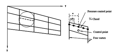
|
| Figure 1. Lift surface |
The expression for the unsteady part of the aerodynamic influence coefficient is:
|
|
(5) |
When the numerator of the integrand function in the above equation is approximated by a fourth-order polynomial, it can be obtained:
|
|
(6) |
where, , , , , , , , , , and are undetermined coefficients. To determine these coefficients, and of the five points is required, located separately in in Figure 1.
The undetermined coefficient is:
|
|
(7a) |
|
|
(7b) |
|
|
(7c) |
|
|
(7d) |
|
|
(7e) |
By substituting Eq.(7) into Eq.(5), the unsteady part can be determined, and then the amplitude array of the element pressure coefficient can be determined based on Eq.(4). Given the Mach number and reduced frequency , where . is the velocity and is the reference length. The aerodynamic influence coefficient matrix is obtained based on the modified doublet aerodynamic model. Based on the boundary conditions, the dimensionless downwash amplitude of the elements is obtained, and finally the pressure coefficients on each element is obtained. The calculation diagram is shown in Figure 2.
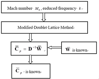
|
| Figure 2. Calculation diagram of modified Doublet Lattice Method |
3. Nonlinear aeroelastic model
The model is shown in Figure 3. For a folding wing with hinge free-play, the dynamic characteristics of the structure also change with the change of free-play. Although free-play nonlinear degrees of freedom account for a small portion of the total degrees of freedom of the structure, they affect the dynamic characteristics of the entire structure. And the corresponding unsteady aerodynamic forces also need to be recalculated. Therefore, when establishing a nonlinear structural dynamics model for folding wings, the mode synthesis method is used to establish a nonlinear structural dynamics model [21]. The more details about the folding wing can be found in Li et al. [21].
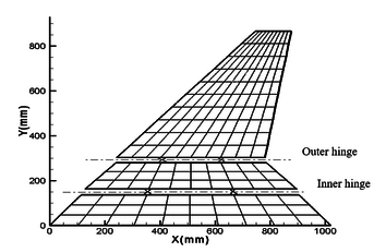
|
| Figure 3. Finite element model for a folding wing (X represent hinges position) [21] |
3.1 Nonlinear structural dynamic model
The mode synthesis method is used to establish a nonlinear structural dynamics model, and the specific nonlinear structural dynamics modeling can be referred to in Li et al. [21]. The final structural dynamics model is:
|
|
(8) |
where, is the modal mass matrix, is the modal stiffness matrix, and is the nonlinear constraint force. The relevant elements can be referred to in Li et al. [21].
3.2 Rational function approximation to modified Doublet Lattice Method
The aerodynamic coefficient matrix obtained by using the modified Doublet Lattice Method is derived under the assumption of harmonic oscillation, therefore it is an aerodynamic force in the frequency domain and cannot be used for dynamic response analysis under any motion situation in the time domain. At present, the process of directly calculating unsteady aerodynamic forces under any motion in the time domain is relatively complex. Therefore, the commonly used method is to use a series of discrete unsteady aerodynamic forces at reduced frequencies in the frequency domain, extend them to the Laplace domain, and use the Laplace variable as the independent variable to represent the time domain unsteady aerodynamic forces in the form of a rational function. This is also a practical approximation method in engineering, and this extension is called the Rational Function Approximation. This approximate form of rational function was first proposed by Jones [22] to fit the Theodorsen function, but the resulting form is relatively complex. Finally, through the development of some scholars [23-25], the commonly used approximate form of unsteady aerodynamic rational functions has been formed.
The biggest advantage of the minimum state approximation method is that fewer aerodynamic states are introduced, resulting in lower order aeroelastic equations in the state space and higher fitting accuracy. The form of the minimum state approximation method is:
|
|
(9) |
where, , , , and are the unknown real matrix to be solved can be iteratively solved using the least squares method, and is the identity matrix
|
(10) |
Then the minimum state approximation will become the Roger approximation. It can be seen that the dimension of is higher. So more aerodynamic state variables are needed. In the minimum state approximation method, can be written:
|
|
(11) |
The number of aerodynamic state variables is N-2. If is instead of in Eq.(9), Eq.(9) can be rewritten as:
|
|
(12) |
And by separating the real and imaginary parts, we can obtain:
|
|
(13) |
|
|
(14) |
For a given reduced frequency , , the following can be obtained from Eqs. (13) and (14):
|
|
(15) |
|
|
(16) |
In the minimum state approximation method, the elements in the matrix and are interrelated. Obviously, it is impossible to determine the matrix to be solved in the form of solving equations. The usual approach is:
(1) is predetermined and its elements are usually distinct and negative;
(2) Given an initial value matrix , and the rank of the matrix cannot be zero;
(3) Apply steady aerodynamic data to form constraint conditions and begin iteration;
(4) Solve the least squares problem of , , ;
(5) Based on obtained in the previous step, , , are recalculated. Then, the fitting error is calculated, and the accuracy is verified. If it does not meet the requirements, the steps are repeated until the accuracy requirements are met.
For the estimation of matrices , , and , the following methods can be used. When the matrix is known, for a given reduced frequency , , the matrix equation about , , can be obtained using the following equation:
|
|
(17) |
where,
|
Due to the unequal rows and columns in Eq.(17), the least squares solution of , , obtained by left multiplying on the left and right sides of the above equation is:
|
|
(18) |
When the matrix is known, for a given reduced frequency , , the matrix equation for , , can be obtained using the following equation:
|
|
(19) |
where,
|
|
Due to the fact that the matrix in Eq.(19) is still not a square matrix, the least squares solution of , , obtained by multiplying on both sides of the equation to the right simultaneously is:
|
|
(20) |
All unknown matrices of the minimum state approximation method have been obtained, allowing for the calculation of unsteady aerodynamic forces in the time domain for dynamic response calculations.
3.3 Aeroelastic equation in state space
The aeroelastic equation for the folding wing is:
|
|
(21) |
where, is the transform matrix.
Note that when is changed, the modal matrices used by each substructure are not affected and is not necessary to be recalculated, simplifying the process of solving nonlinear equations. In Eq.(21), the nonlinear constraint contained in is the nonlinear function of the generalized displacement at the hinge connection, i.e. the elastic connection. In existing research, the treatment method for nonlinear free-play problems is generally to express nonlinear forces in segmented form and introduce them into dynamic equations for solution. Assuming is a generalized displacement at the hinge, the free-play nonlinearity is modeled using the model in Bae et al. [26], and its moment is shown in Figure 4. Meanwhile, friction is inevitable at the hinge connection, and that friction can serve as a stability factor is demonstrated in Sinha and Griffin [27]. Therefore, in order to weaken the various nonlinear motions of folding wings under free-play conditions, friction moment is used to weaken the influence of free-play nonlinearity.
| ||||
| Figure 4. Structural nonlinear diagram |
The expression for free-play nonlinearity is:
|
|
(22) |
where, is the free-play. When , the moment is the linear function of .
The expression for frictional nonlinearity is:
|
|
(23) |
The non-linear characteristic of this friction is that when is small, the friction moment is equal to the product of the friction stiffness and the deflection angle . When the moment is greater than , the friction stiffness is 0, and the friction moment remains constant. Introducing frictional nonlinearity with respect to four independent nonlinear degrees of freedom into the nonlinear aeroelastic motion equation of free-play can achieve the analysis of free-play and frictional nonlinear aeroelastic response.
Here, introducing aerodynamic state variables , the minimum state method is used to approximate the rational function of frequency domain aerodynamics, the state space form of the aeroelastic equation is:
|
|
(24) |
where, , , . , , , and , which are all unknown matrices in the minimum state approximation. is the aerodynamic lag matrix, and is the reference length.
4. Analysis and discussion
Only the nonlinear aeroelastic response of the folding wing in the fully unfolded state has been analyzed here. The mass matrix and stiffness matrix of each substructure of the folding wing are obtained through DMAP language. The modified Doublet Lattice Method is used to obtain the unsteady aerodynamic forces of a folding wing in the frequency domain, and the expression of the aeroelastic equation in the state space is obtained through the minimum state approximation. For each substructure, six vibration modes are retained, and 10 degrees of freedom are coupled to each other through MPC and torsion springs at the interface, while 2 independent nonlinear degrees of freedom are retained. The final dynamic equation of the folding wing obtained is 22. After introducing 4 aerodynamic state variables, the aeroelastic equation in the state space is finally obtained, that is, Eq.(24) is 48, Finally, the time-domain aeroelastic response of the folding wing is obtained using the Runge-Kutta method in MATLAB.
4.1 Aerodynamic model validation
To verify the correctness of the modified Doublet Lattice Method, two examples are presented here.
Example 1: In Qian [29], an example is given to calculate the lift and lift coefficient of a swept wing. Its aspect ratio is 5 and the taper ratio is 1, as shown in Figure 5. Take its aspect as 5, root chord as 1, leading edge sweep angle as , Mach number , . When the frequency is zero, the modified Doublet Lattice Method will degenerate into the vortex lattice method, which is the steady part of the modified Doublet Lattice Method. The lift and lift coefficient of the swept wing are obtained using the steady part, and the comparison results are shown in Table 1.
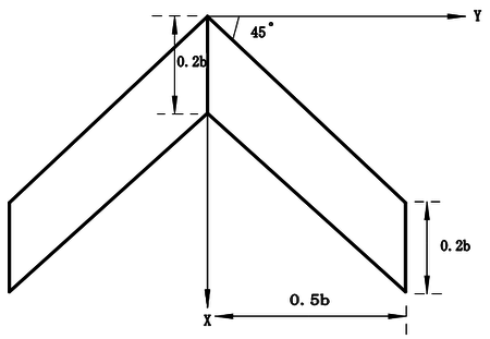
|
| Figure 5. Wing geometry dimensions |
| Qian [29] | Present | Relative error (%) | |
|---|---|---|---|
| Lift ( ) | 848.554 | 851.296 | 0.323 |
| Lift Coefficient | 0.059921 | 0.0601131 | 0.321 |
Example 2: In Zhao [15], a swept wing with equal chord length, leading edge sweep angle , half span length , aspect ratio , as shown in Figure 6. There is a control surface at 50% of the half span length, with the chord length of the control surface being of the chord length c of the wing, and the amplitude of the control surface oscillates harmoniously. Reduced frequency , Mach number . Using the correction method, the changes in the real and imaginary parts of the pressure coefficients of the chord distribution units with a half span length of 42.5% and a half span length of 72.5% are shown in Figure 7.
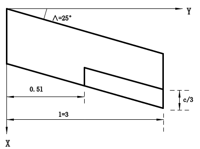
|
| Figure 6. Swept wing with equal chord length |
In Example 1, four elements are used for both the left and right wings. The modified Doublet Lattice Method is reduced to zero frequency and degenerated into the vortex lattice method, which uses the steady part of the modified Doublet Lattice Method to obtain lift and lift coefficients. The relative error is within an acceptable range. In Example 2, the trend of the results obtained using the modified Doublet Lattice Method is basically similar to the trend of the results in Zhao [15]. Due to the sparsity of the element, the obtained curve is not smooth enough. By further increasing the number of elements in the chord and spanwise directions, this result can be improved. Comparing the chordal distribution of pressure coefficients at different spans, it can be seen that compared to the pressure coefficient distribution at 42.5% half span, the distribution at 72.5% half span has a significant change, mainly due to the deflection angle of the control surface, making the pressure coefficient distribution at the trailing edge more prominent. From the above two examples, it can be seen that the modified Doublet Lattice Method is correct.
Based on the modified Doublet Lattice Method, frequency domain unsteady aerodynamic calculations on folding wings is performed. Furthermore, the minimum state approximation method is used to fit the unsteady aerodynamic forces. The discrete form of the generalized aerodynamic force obtained in the frequency domain is given a lag matrix in advance. The real and imaginary parts of the generalized aerodynamic force matrix at 15 reduced frequency points are fitted. And , , , are known, and then the steady-state aerodynamic force data is used to form constraint conditions for iteration. Here are some fitting results, as shown in Figure 8. It can be seen that the approximate value matches the exact value well, and after obtaining the unknown matrix in the minimum state approximation, time-domain aeroelastic analysis can be achieved.
| ||||||||||||
| Figure 8. Minimum state approximation results for unsteady aerodynamics of folding wings |
4.2 Structural nonlinear aeroelastic analysis
According to Li et al. [21], it can be seen that when , the model is equal to the linear model. And the linear flutter velocity . The , , of the inner and outer hinges are taken as examples. An initial disturbance of 0.01mm is added to the normal direction of the trailing edge node of the wing tip to obtain the velocity at which the normal displacement response of the leading edge of the folding wing tip begins to diverge. Assuming , the different moments are introduced separately, the displacement response obtained are shown in Figures 9 and 10.
| ||||||||
| Figure 9. Friction at the inner hinge | ||||||||
| ||||||||
| Figure 10. Friction at the outer hinge | ||||||||
From Figures 9 and 10, it can be seen that when the friction stiffness is constant, an appropriate friction moment can suppress the divergence of displacement. Friction nonlinearity can effectively weaken the divergent motion of the normal displacement of the leading edge node of the wing tip, transforming it from an unstable motion tending towards divergence to a limit cycle motion with limited amplitude. It can be observed that the normal displacement response of the wingtip is centered around the zero position. This is because both free-play nonlinearity and friction nonlinearity are centrally symmetric, and after superposition, they remain centrally symmetric. This result also verifies the correctness of the model proposed in this paper.
In order to further clarify the influence of physical parameters of friction nonlinearity on the nonlinear aeroelasticity of free-play, the effects of moment and frictional stiffness on the response of free-play nonlinear aeroelastic systems are analyzed. Taking the free-play between the inner and outer hinges as an example, the displacement tends to diverge at a speed of and , the effect of frictional nonlinearity on the aeroelasticity of the free-play is shown in Figure 11.
| ||||
| Figure 11. Influence of nonlinear friction on free-play aeroelasticity |
From Figure 11, it can be seen that as the initial moment increases, the amplitude of the wingtip normal displacement decreases. As the friction stiffness increases, the amplitude of normal displacement at the leading edge of the wing tip does not change significantly. In Figure 11(a), , as the initial moment increases, increases. When reaches a certain degree, the effect of the initial moment and the external moment caused by free-play nonlinearity is opposite, weakening the free-play nonlinearity. In Figure 11(b), , as the friction stiffness increases, decreases. In a smaller displacement range, plays a major role, so the initial moment still plays a major role in a larger displacement range. This phenomenon indicates that compared to frictional stiffness, frictional moment plays an important role in reducing response amplitude. At the same time, when friction nonlinearity is added to the free-play nonlinearity at the outer hinge, the normal amplitude of the wing tip is always larger than when friction nonlinearity is added to the free-play nonlinearity at the inner hinge. In summary, to a certain extent, frictional nonlinearity can effectively reduce vibration amplitude, which is beneficial nonlinearity.
5. Conclusions
The structural nonlinear aeroelastic analysis of folding wings is conducted by the modified Doublet Lattice Method. Firstly, a modified Doublet Lattice Method is studied to relax the aspect ratio limitation of aerodynamic elements, and its correctness is verified through numerical examples. Secondly, the rational function approximation method is discussed, and the modified Doublet Lattice Method is approximated using the minimum state method to obtain the unsteady aerodynamic forces in the time domain. Finally, the aeroelastic characteristics of a folding wing with free-play and friction nonlinearities are studied by combining time-domain unsteady aerodynamics and nonlinear structural dynamics models. The following conclusions can be drawn:
(1) The modified Doublet Lattice Method that relaxes the aspect ratio limitation of aerodynamic elements is feasible and effective, which improves the accuracy of the aerodynamic influence coefficient matrix. At the same time, it can reduce the constraints on the aerodynamic element, thereby saving calculation time and providing conditions for rapid aerodynamic calculations;
(2) It has been proven through simulations that friction can suppress the influence of free-play nonlinearity on aeroelastic response. For the aerodynamic elastic response with free-play nonlinearity, adding friction can effectively weaken the nonlinear strength of the free-play of the folding wing.
(3) Friction moment plays an important role in reducing response amplitude and is a beneficial nonlinearity.
Funding: This research is supported by Natural Science Basic Research Plan in Shaanxi Province of China (2021JQ-847 and 2023-JC-YB-076).
References
[1] Chen S.S., Jia M.L., Liu Y.X., et al. Development status on deformation modes and key technologies of aerodynamic layout design about morphing aircraft (in Chinese). Acta Aeronautica et Astronautica Sinica, 45(5), 629595, 2024.
[2] Ma H., Song B.F., Zhou Z.B., Zhang D.S.H.Analysis of the development status of multi-section morphing wing technology (in Chinese).Tactical Missile Technology, 2024. https://doi.org/10.16358/j.issn.1009-1300.20230121, 2024-02-08.
[3] Snyder M.P., Sanders B., Eastep F.E., Frank G.J. Vibration and flutter characteristics of a folding wing. Journal of Aircraft, 46(3):791-799, 2009.
[4] Wang I., Gibbs S.C., Dowell E.H. Aeroelastic model of multisegmented folding wings:Theory and experiment. Journal of Aircraft, 49(3)911-921, 2012.
[5] Lee D.H., Weisshaar T.A. Aeroelastic studies on a folding wing configuration. 46th AIAA/ ASME/ASCE/AHS/ASC Structures, Structural Dynamics and Materials Conference, Austin, Texas, 2005.
[6] Lee D.H., Chen P.C. Nonlinear aeroelastic studies on a folding wing configuration with free play hinge nonlinearity. 47th AIAA/ASME/ASCE/AHS/ASCStructures, Structural Dynamics and Materials Conference, Newport, Rhode Island, 2006.
[7] Attar P., Tang D., Dowell E.H. Nonlinear aeroelastic study for folding wing structures. AIAA Journal, 48(10)2187-2195, 2010.
[8] Reich G.W., Bowman J.C., Sanders B., et al. Development of an integrated aeroelastic multibody morphing simulation tool. 47th AIAA/ASME/ASCE/AHS/ASC Structures, Structural Dynamics and Materials Conference, Newport, Rhode Island, 2006.
[9] Zhao Y.H., Hu H.Y. Parameterized aeroelastic modeling and flutter analysis for a folding wing. Journal of Sound Vibration, 331:208-324, 2012.
[10] Tang D., Dowell E.H. Theoretical and experimental aeroelastic study for folding wing structures. Journal of Aircraft, 45(4):1136-1147, 2008.
[11] Hu W., Yang Z., Gu Y., Wang X. The nonlinear aeroleastic characteristics of a folding wing with cubic stiffness. Journal of Sound and Vibration, 400:22-39, 2017.
[12] Ni Y.G., Zhang W., Lv Y. Fast structural dynamic modeling and analysis for horizontally folding wing. Revista Internacional de Métodos Numéricos para Cálculo y Diseño en Ingeniería, 37(3), 35, 2021.
[13] Ni Y.G., Zhang W., Lv Y.. Multi-body dynamics modeling and transient characteristics analysis for a folding wing. Revista Internacional de Métodos Numéricos para Cálculo y Diseño en Ingeniería, 37(1), 4, 2021.
[14] Yang N., Wu Zh.G., Yang Ch., Cao Q.K. Flutter analysis of a folding wing with structural nonlinearity. Engineeing Mechanics, 29(2):197-204, 2012.
[15] Zhao Y.H. Aeroelasticity and control. Science Press, Beijing, 2007.
[16] Verstraete M.L., Preidikman S., Roccia B.A., Mook D.T. A numerical nodel to study the nonlinear and unsteady aerodynamics of bioinspired morphing-wing comcepts. International Journal of Micro Air Vehicles, 7(3):327-345, 2015.
[17] Albano E., Rodden W.P. A doublet-lattice method for calculating lift distributions on oscillating surfaces in subsonic flows. AIAA Journal, 7(2):279-285, 1969.
[18] Landabl M.T. Kernel function for nonplanar oscillating surfaces in a subsonic flow. AIAA Journal, 5(5):1045-1046, 1967.
[19] Rodden W.P., Giesing J.P., Kalman T.P. Refinement of the nonplanar aspects of the subsonic doublet-lattice lifting surface method. Journal of Aircraft, 9(1):69-73, 1972.
[20] Rodden W.P., Taylor P.F., Mcintosh S.C. Further refinement of the subsonic doublet-dattice method. Journal of Aircraft, 35(5):720-727, 1998.
[21] Li P.CH., Ni Y.G., Hou Ch., Wan X.P., Zhao M.Y. Nonlinear aeroelastic aodeling of a folding wing structure. Journal of Physics: Conf. Series, 1215, 012009, 2019
[22] Jones R.T. The unsteady lift of a wing of finite aspect ratio. NACA Report-681, 1941.
[23] Roger K.L. Airplane math modeling methods for active control design. AGARD-CP, 228:4.1-4.11, 1977.
[24] Karpel M. Extensions to the minimum-state aeroelastic modeling method. AIAA Journal, 29(11):2007-2009, 1991.
[25] Vepa R. Finite state modeling of aeroelastic systems. NASA CR-2779, 1977.
[26] Bae J.S., Inman D.J., Lee I. Effects of structural nonlinearity on subsonic aeroelastic characteristcs of an aircraft wing with control surface. Journal of Fluids and Structures, 19(6):747-763, 2004.
[27] Sinha A., Griffin J.H. Effects of friction dampers on aerodynamically unstable rotor stages. AIAA Journal, 23(2):262-270, 1985.
[28] Liu B.H., Li M., Tan T.C. Flutter study of a two-dimensional airfoil with structural nonlinearities. Engineering Mechanics, 30(4):448-454, 2013.
[29] Qian Y.J. Aerodynamics. Beijing University of Aeronautics and Astronautics Press, Beijing, 2004.Document information
Published on 12/07/24
Accepted on 15/06/24
Submitted on 03/03/24
Volume 40, Issue 3, 2024
DOI: 10.23967/j.rimni.2024.06.004
Licence: CC BY-NC-SA license
Share this document
Keywords
claim authorship
Are you one of the authors of this document?
