| (29 intermediate revisions by 2 users not shown) | |||
| Line 13: | Line 13: | ||
==Abstract== | ==Abstract== | ||
| − | To develop a precise neural network model designed for segmenting ultrasound images of thyroid nodules. The deep learning U-Net network model was utilized as the main backbone, with improvements made to the convolutional operations and the implementation of multilayer perceptron modeling at the lower levels, using the more effective BCEDice loss function. The modified network achieved enhanced segmentation precision and robust generalization capabilities, with a Dice coefficient of 0.9062, precision of 0.9153, recall of 0.9023, and an | + | To develop a precise neural network model designed for segmenting ultrasound images of thyroid nodules. The deep learning U-Net network model was utilized as the main backbone, with improvements made to the convolutional operations and the implementation of multilayer perceptron modeling at the lower levels, using the more effective <math display="inline">\mathsf{BCEDice}</math> loss function. The modified network achieved enhanced segmentation precision and robust generalization capabilities, with a <math>\mathsf{Dice}</math> coefficient of 0.9062, precision of 0.9153, recall of 0.9023, and an <math display="inline"> F_1 </math> score of 0.9062, indicating improvements over the U-Net and Swin-Unet to various extents. The U-Net network enhancement presented in this study outperforms the original U-Net across all performance indicators. This advancement could help physicians make more precise and efficient diagnoses, thereby minimizing medical errors. |
'''Keywords''': U-Net, image segmentation, thyroid nodule ultrasound imaging, deep learning | '''Keywords''': U-Net, image segmentation, thyroid nodule ultrasound imaging, deep learning | ||
| Line 23: | Line 23: | ||
Although thyroid nodule ultrasound imaging technology is mature, the quality of imaging cannot be guaranteed, and shortcomings such as blurred edges of thyroid nodules in images are unavoidable. Differences in the model and type of ultrasound equipment also lead to significant differences in the collected ultrasound images. Additionally, fine-needle aspiration biopsy surgery requires a large amount of medical and human resources and is somewhat invasive for patients. Therefore, this diagnostic method heavily relies on the subjective judgment of attending physicians, which can easily lead to misdiagnosis due to differences in doctors’ operational experience and techniques. Unnecessary biopsy surgeries can also cause patients more suffering. Therefore, improving the accuracy of segmentation for ultrasound images of thyroid nodules in computational fields will notably enhance the precision and efficacy of clinical diagnosis and treatment. | Although thyroid nodule ultrasound imaging technology is mature, the quality of imaging cannot be guaranteed, and shortcomings such as blurred edges of thyroid nodules in images are unavoidable. Differences in the model and type of ultrasound equipment also lead to significant differences in the collected ultrasound images. Additionally, fine-needle aspiration biopsy surgery requires a large amount of medical and human resources and is somewhat invasive for patients. Therefore, this diagnostic method heavily relies on the subjective judgment of attending physicians, which can easily lead to misdiagnosis due to differences in doctors’ operational experience and techniques. Unnecessary biopsy surgeries can also cause patients more suffering. Therefore, improving the accuracy of segmentation for ultrasound images of thyroid nodules in computational fields will notably enhance the precision and efficacy of clinical diagnosis and treatment. | ||
| − | Addressing thyroid nodule segmentation, the U-Net model, as introduced by Ronneberger et al. [3], revolutionized deep learning techniques for medical image segmentation by integrating skip connections within its encoder-decoder architecture. This advancement marked a significant milestone, heralding a new era in the field. In a parallel development, Ma et al. [4] improved the network by introducing a multi-dilation convolutional block. This enhancement enables more accurate segmentation of nodule regions, resulting in the creation of more precise binary masks for medical image segmentation. Hu | + | Addressing thyroid nodule segmentation, the U-Net model, as introduced by Ronneberger et al. [3], revolutionized deep learning techniques for medical image segmentation by integrating skip connections within its encoder-decoder architecture. This advancement marked a significant milestone, heralding a new era in the field. In a parallel development, Ma et al. [4] improved the network by introducing a multi-dilation convolutional block. This enhancement enables more accurate segmentation of nodule regions, resulting in the creation of more precise binary masks for medical image segmentation. Hu et al. [5] introduced attention mechanisms for thyroid nodule segmentation, optimizing low-dimensional features of images and preserving important features through the fusion of high and low-dimensional features. Sun et al. [6] fused different feature layers with the U-Net as the backbone network and introduced SE attention mechanisms to further improve segmentation accuracy. Chu et al. [7] introduced a thyroid nodule segmentation network utilizing U-Net architecture, substantially enhancing segmentation accuracy with limited datasets, thereby effectively aiding physicians in diagnosing thyroid nodules. Oktay et al. [8] introduced the Attention-UNet, a novel network model designed to automatically prioritize targets of diverse sizes and shapes. This approach effectively accentuates significant features while mitigating attention towards irrelevant areas. Zhou et al. [9] developed the Deeply Supervised Encoder-Decoder UNet++ network. This diminishes the semantic disparity between the feature maps of encoder and decoder subnetworks. Meanwhile, Chen et al. [10] enhanced the DeepLabv3+ model by integrating a decoder module to refine segmentation outcomes and integrating depth-wise separable convolutions into both the spatial pyramid pooling and decoder modules. Badrinarayanan et al. [11] introduced the SegNet segmentation network. It symmetrically performs downsampling and upsampling. Many models adopt multi-stage segmentation methods, further increasing computational complexity, indicating the need to improve the segmentation speed of many thyroid nodule models. |
Currently, the widely used deep learning neural network in medical imaging is the U-Net network. However, U-Net still faces limitations in thyroid nodule segmentation, such as ineffective utilization of pixel-space information and long training times. The primary contribution of this paper is the research and development of an optimal network structure designed to accurately segment nodules in the thyroid region. | Currently, the widely used deep learning neural network in medical imaging is the U-Net network. However, U-Net still faces limitations in thyroid nodule segmentation, such as ineffective utilization of pixel-space information and long training times. The primary contribution of this paper is the research and development of an optimal network structure designed to accurately segment nodules in the thyroid region. | ||
| Line 55: | Line 55: | ||
{| class="wikitable" style="margin: 0em auto 0.1em auto;border-collapse: collapse;width:auto;" | {| class="wikitable" style="margin: 0em auto 0.1em auto;border-collapse: collapse;width:auto;" | ||
|-style="background:white;" | |-style="background:white;" | ||
| − | |style="text-align: center;padding:10px;"| [[Image:Draft_Xu_795668614-image2.png| | + | |style="text-align: center;padding:10px;"| [[Image:Draft_Xu_795668614-image2.png|600px]] |
|- | |- | ||
| style="background:#efefef;text-align:left;padding:10px;font-size: 85%;"| '''Figure 2'''. Swin-UNet network architecture diagram | | style="background:#efefef;text-align:left;padding:10px;font-size: 85%;"| '''Figure 2'''. Swin-UNet network architecture diagram | ||
|} | |} | ||
| − | |||
==3. Improved U-Net network== | ==3. Improved U-Net network== | ||
| Line 68: | Line 67: | ||
{| class="wikitable" style="margin: 0em auto 0.1em auto;border-collapse: collapse;width:auto;" | {| class="wikitable" style="margin: 0em auto 0.1em auto;border-collapse: collapse;width:auto;" | ||
|-style="background:white;" | |-style="background:white;" | ||
| − | |style="text-align: center;padding:10px;"| [[Image:Draft_Xu_795668614-image3.png| | + | |style="text-align: center;padding:10px;"| [[Image:Draft_Xu_795668614-image3.png|600px]] |
|- | |- | ||
| style="background:#efefef;text-align:left;padding:10px;font-size: 85%;"| '''Figure 3'''. Schematic of the improved U-Net network structure | | style="background:#efefef;text-align:left;padding:10px;font-size: 85%;"| '''Figure 3'''. Schematic of the improved U-Net network structure | ||
| Line 167: | Line 166: | ||
1. Depth-wise separable convolution is advantageous for encoding positional information of features. Experimental results indicate that convolutional layers in MLPs are sufficient for encoding positional information and outperform standard positional encoding in practical performance. | 1. Depth-wise separable convolution is advantageous for encoding positional information of features. Experimental results indicate that convolutional layers in MLPs are sufficient for encoding positional information and outperform standard positional encoding in practical performance. | ||
| − | 2. DWConv has fewer parameters | + | 2. DWConv has fewer parameters. In the tokenized MLP stage, the features are initially transformed and projected onto tokens, with the channel count adjusted to match the number of tokens. |
The computational process of the tokenized MLP stage module involves: | The computational process of the tokenized MLP stage module involves: | ||
| Line 219: | Line 218: | ||
Similar to most U-shaped network structures, skip connection operations fuse the feature information of downsampling and upsampling, effectively reducing information loss during downsampling to achieve better thyroid nodule segmentation. | Similar to most U-shaped network structures, skip connection operations fuse the feature information of downsampling and upsampling, effectively reducing information loss during downsampling to achieve better thyroid nodule segmentation. | ||
| − | =4. Experiment and | + | ==4. Experiment and results== |
| − | ==4.1 Experimental | + | ===4.1 Experimental dataset=== |
The thyroid nodule ultrasound scan images used in this study are sourced from the publicly available TN3K (thyroid nodule 3 thousand) dataset (Gong et al., 2021), which includes 3493 ultrasound images with pixel labels. The dataset comprises high-quality nodule mask annotations from various devices and views. | The thyroid nodule ultrasound scan images used in this study are sourced from the publicly available TN3K (thyroid nodule 3 thousand) dataset (Gong et al., 2021), which includes 3493 ultrasound images with pixel labels. The dataset comprises high-quality nodule mask annotations from various devices and views. | ||
| − | ==4.2 Experimental | + | ===4.2 Experimental design=== |
| − | The experimental setup includes the following parameters: image dimensions are uniformly adjusted to | + | The experimental setup includes the following parameters: image dimensions are uniformly adjusted to <math display="inline">256\times 256\times 1</math>, with an initial learning rate set at 0.0005, and a batch size of 8. The Adam optimizer is employed for model optimization. The models undergo training across over a span of 100 epochs. |
| − | The BCE loss function treats each pixel as an independent binary classification problem, calculating the loss for each pixel. It offers good and stable focus on individual pixels. While the Dice loss function demonstrates excellent experimental performance for small target objects, maintaining stable training results is challenging. Based on the above studies, this paper aims to balance stability and accuracy in thyroid nodule segmentation training. Therefore, the BCEDiceLoss is utilized during training, combining the advantages of both loss functions to achieve better experimental results. | + | The <math>\mathsf{BCE}</math> loss function treats each pixel as an independent binary classification problem, calculating the loss for each pixel. It offers good and stable focus on individual pixels. While the <math>\mathsf{Dice}</math> loss function demonstrates excellent experimental performance for small target objects, maintaining stable training results is challenging. Based on the above studies, this paper aims to balance stability and accuracy in thyroid nodule segmentation training. Therefore, the <math>\mathsf{BCEDiceLoss}</math> is utilized during training, combining the advantages of both loss functions to achieve better experimental results. |
| − | The BCE (Binary Cross-Entropy) loss function is defined as follows: | + | The <math>\mathsf{BCE}</math> (Binary Cross-Entropy) loss function is defined as follows: |
| − | {| class="formulaSCP" style="width: 100%; text-align: center;" | + | |
| + | {| class="formulaSCP" style="width: 100%; text-align: left;" | ||
| + | |- | ||
| + | | | ||
| + | {| style="text-align: center; margin:auto;width: 100%;" | ||
|- | |- | ||
| − | | <math>\mathcal{L}_{\ | + | | style="text-align: center;" | <math> \mathcal{L}_{\mathsf{BCE}}(X,Y,\widehat{Y})^{\leftrightarrow}=\frac1P\sum_{\mathsf{ij}}-(R_{ij}\log(P_{ij}))+(1-R_{ij})\log{(1-P_{ij})}) </math> |
| − | |(10) | + | |} |
| + | | style="width: 5px;text-align: right;white-space: nowrap;" |(10) | ||
|} | |} | ||
| − | In | + | In Eq. (10), <math display="inline"> X </math> represents the initial thyroid nodule image, <math display="inline"> Y </math> the true labels, and <math display="inline">\hat{Y}</math> the corresponding predicted labels. |
| − | The Dice loss function is defined as: | + | The <math>\mathsf{Dice}</math> loss function is defined as: |
| − | {| class="formulaSCP" style="width: 100%; text-align: | + | |
| + | {| class="formulaSCP" style="width: 100%; text-align: left;" | ||
|- | |- | ||
| − | | <math>\mathcal{L}_{\ | + | | |
| − | |(11) | + | {| style="text-align: center; margin:auto;width: 100%;" |
| + | |- | ||
| + | | style="text-align: center;" | <math> \mathcal{L}_{\mathsf{Dice}}(X,Y,\widehat{Y})=1-\frac{\displaystyle\sum_{ij}P_{ij}R_{ij}+\varepsilon}{\displaystyle\sum_{ij}\left(P_{ij}+R_{ij}\right)-\displaystyle\sum_{ij}P_{ij}R_{ij}+\varepsilon} </math> | ||
| + | |} | ||
| + | | style="width: 5px;text-align: right;white-space: nowrap;" |(11) | ||
|} | |} | ||
| + | In Eq. (11), <math>\varepsilon</math> represents a smoothing coefficient, which prevents situations like zero denominators. The computation of <math display="inline">\mathsf{BCEDiceLoss}</math> is as follows: | ||
| − | + | {| class="formulaSCP" style="width: 100%; text-align: left;" | |
| − | + | ||
| − | + | ||
| − | {| class="formulaSCP" style="width: 100%; text-align: | + | |
|- | |- | ||
| − | | <math> | + | | |
| − | |(12) | + | {| style="text-align: center; margin:auto;width: 100%;" |
| + | |- | ||
| + | | style="text-align: center;" | <math> {L}_{\mathsf{BCEDice}}=\alpha {L}_{\mathsf{BCE}}+\left( 1-\alpha \right) {L}_{\mathsf{Dice}} </math> | ||
| + | |} | ||
| + | | style="width: 5px;text-align: right;white-space: nowrap;" |(12) | ||
|} | |} | ||
| − | |||
| − | =5. Results and | + | ==5. Results and discussion== |
| − | == | + | ===5.1 Evaluation metrics=== |
| − | The evaluation metrics employed include the Dice coefficient, precision (P), recall (R), and | + | The evaluation metrics employed include the <math display="inline">\mathsf{Dice}</math> coefficient, precision (<math display="inline">P</math>), recall (<math display="inline">R</math>), and <math display="inline">F_1</math>-score. The <math display="inline">\mathsf{Dice}</math> coefficient measures the similarity between sets. Values for the <math display="inline">\mathsf{BCE}</math> loss function fall within the range of 0 to 1, with higher values denoting improved segmentation performance achieved by the model. Precision, recall, and <math display="inline">F_1</math>-score provide additional insights into the accuracy and reliability of the segmentation. |
| − | The formula for calculating the Dice coefficient is as follows: | + | The formula for calculating the <math display="inline">\mathsf{Dice}</math> coefficient is as follows: |
| − | {| class="formulaSCP" style="width: 100%; text-align: | + | |
| + | {| class="formulaSCP" style="width: 100%; text-align: left;" | ||
|- | |- | ||
| − | | <math>Dice=\frac{2\left| A\cap B\right| }{\left| A\right| +\left| B\right| } | + | | |
| − | |(13) | + | {| style="text-align: center; margin:auto;width: 100%;" |
| + | |- | ||
| + | | style="text-align: center;" | <math> \mathsf{Dice}=\frac{2\left| A\cap B\right| }{\left| A\right| +\left| B\right| } </math> | ||
| + | |} | ||
| + | | style="width: 5px;text-align: right;white-space: nowrap;" |(13) | ||
|} | |} | ||
| − | In | + | In Eq. (13), <math display="inline"> A </math> and <math display="inline"> B </math> represent the actual and predicted areas of the image, respectively. |
| − | The formulas for calculating precision (P), recall (R), and the | + | The formulas for calculating precision (<math display="inline">P</math>), recall (<math display="inline">R</math>), and the <math display="inline">F_1</math>-score are as follows: |
| − | + | {| class="formulaSCP" style="width: 100%; text-align: left;" | |
| − | {| class="formulaSCP" style="width: 100%; text-align: | + | |
|- | |- | ||
| − | | <math> | + | | |
| − | |(14) | + | {| style="text-align: center; margin:auto;width: 100%;" |
| + | |- | ||
| + | | style="text-align: center;" | <math> P=\frac{{T}_{P}}{{T}_{P}+{F}_{P}} </math> | ||
| + | |} | ||
| + | | style="width: 5px;text-align: right;white-space: nowrap;" |(14) | ||
|} | |} | ||
| − | |||
| − | + | {| class="formulaSCP" style="width: 100%; text-align: left;" | |
| − | {| class="formulaSCP" style="width: 100%; text-align: | + | |
|- | |- | ||
| − | | | + | | |
| − | + | {| style="text-align: center; margin:auto;width: 100%;" | |
| − | + | ||
| − | + | ||
| − | {| | + | |
|- | |- | ||
| − | | <math>\ | + | | style="text-align: center;" | <math> R=\frac{{T}_{P}}{{T}_{P}+{F}_{N}} </math> |
| − | |( | + | |} |
| + | | style="width: 5px;text-align: right;white-space: nowrap;" |(15) | ||
|} | |} | ||
| − | + | {| class="formulaSCP" style="width: 100%; text-align: left;" | |
| − | + | ||
| − | + | ||
| − | + | ||
| − | + | ||
| − | + | ||
| − | + | ||
| − | + | ||
| − | + | ||
| − | + | ||
|- | |- | ||
| − | | | + | | |
| − | + | {| style="text-align: center; margin:auto;width: 100%;" | |
| − | + | ||
| − | + | ||
| − | + | ||
| − | + | ||
| − | | | + | |
| − | + | ||
| − | + | ||
| − | + | ||
| − | + | ||
|- | |- | ||
| − | | | + | | style="text-align: center;" | <math> {F}_{1}=2\times \frac{P\times R}{P+R} </math> |
| − | + | |} | |
| − | + | | style="width: 5px;text-align: right;white-space: nowrap;" |(16) | |
| − | | | + | |
| − | | | + | |
| − | | | + | |
| − | + | ||
| − | + | ||
| − | + | ||
| − | + | ||
| − | + | ||
|} | |} | ||
| − | + | ===5.2 Results and analysis=== | |
| − | + | ====5.2.1 Comparing the training effects of different loss functions==== | |
| − | + | The initial set of experiments aims to assess the training effects of the enhanced network model proposed in this paper, employing <math display="inline">\mathsf{BCE}</math>, <math display="inline">\mathsf{Dice}</math>, and <math display="inline">\mathsf{BCEDice}</math> loss functions. | |
| − | + | As shown in [[#tab-1|Table 1]], based on the data analysis provided in the table above, it is apparent that for the enhanced neural network proposed in this paper, when trained using the <math display="inline">\mathsf{BCE}</math> loss function, the <math display="inline">\mathsf{Dice}</math> score is 0.9016, which represents the lowest score among the evaluated functions. However, when the model is trained using the <math display="inline">\mathsf{Dice}</math> loss function, a slight improvement is observed compared to utilizing the <math display="inline">\mathsf{BCE}</math> function, with the <math display="inline">\mathsf{Dice}</math> score increasing to 0.9031. | |
| − | < | + | When combining the <math display="inline">\mathsf{BCE}</math> loss function with the <math display="inline">\mathsf{Dice}</math> loss function for training thyroid nodule ultrasound images, experimental results show that compared to using each loss function individually, the combination of both yields the highest <math display="inline">\mathsf{Dice}</math> coefficient, precision, and score, reaching 0.9062, 0.9153, and 0.9062, respectively. The results suggest that the enhanced U-Net network proposed in this paper demonstrates superior performance in balancing stability and segmentation effectiveness when utilizing the <math display="inline">\mathsf{BCEDice}</math> loss function. |
| − | < | + | |
| − | + | <div class="center" style="font-size: 85%;">'''Table 1'''. Training results with various loss functions</div> | |
| − | + | ||
| − | + | <div id='tab-1'></div> | |
| − | | | + | {| class="wikitable" style="margin: 1em auto 0.1em auto;border-collapse: collapse;font-size:85%;width:auto;" |
| − | + | |-style="text-align:center" | |
| − | + | ! Loss Function !! <math display="inline">\mathsf{Dice}</math> !! <math display="inline"> P </math> !! <math display="inline"> R </math> !! <math>{F}_{1}</math> | |
| − | + | |-style="text-align:center" | |
| − | |- | + | | style="btext-align: center;vertical-align: top;"|<math display="inline">\mathsf{BCE}</math> |
| − | | style=" | + | | style="btext-align: center;vertical-align: top;"|0.9016 |
| − | | style=" | + | | style="btext-align: center;vertical-align: top;"|0.9142 |
| − | | style=" | + | | style="btext-align: center;vertical-align: top;"|0.8959 |
| − | | style=" | + | | style="btext-align: center;vertical-align: top;"|0.9016 |
| − | | style=" | + | |-style="text-align:center" |
| − | + | | style="text-align: center;vertical-align: top;"|<math display="inline">\mathsf{Dice}</math> | |
| − | | style="text-align: center;vertical-align: top;"|< | + | | style="text-align: center;vertical-align: top;"|0.9031 |
| − | | style="text-align: center;vertical-align: top;"| | + | | style="text-align: center;vertical-align: top;"|0.9074 |
| − | | style="text-align: center;vertical-align: top;"| | + | | style="text-align: center;vertical-align: top;"|0.9044 |
| − | | style="text-align: center;vertical-align: top;"| | + | | style="text-align: center;vertical-align: top;"|0.9031 |
| − | | style="text-align: center;vertical-align: top;"| | + | |-style="text-align:center" |
| − | |- | + | | style="text-align: center;vertical-align: top;"|<math display="inline">\mathsf{BCEDice}</math> |
| − | + | | style="text-align: center;vertical-align: top;"|0.9062 | |
| − | | style=" | + | | style="text-align: center;vertical-align: top;"|0.9153 |
| − | | style=" | + | | style="text-align: center;vertical-align: top;"|0.9023 |
| − | | style=" | + | | style="text-align: center;vertical-align: top;"|0.9062 |
| − | | style=" | + | |
|} | |} | ||
| + | ====5.2.2 Comparison of segmentation performance of different networks==== | ||
| − | + | To further assess the effectiveness of the enhanced model presented in the study, the same dataset is used to train three distinct network models: U-Net, Swin-Unet, and the enhanced model. Subsequently, the segmentation accuracy is evaluated. | |
| − | + | Based on [[#tab-2|Table 2]], the <math display="inline">\mathsf{Dice}</math> score of the Swin-Unet network reaches 0.7322, which is the lowest among the evaluated networks. The U-Net network achieves a <math display="inline">\mathsf{Dice}</math> score of 0.8971, presenting a notable improvement of 22.52% compared to Swin-Unet. After optimization, the enhanced neural network proposed in this paper achieves the highest <math display="inline">\mathsf{Dice}</math> value of 0.9062 and the highest accuracy of 0.9153. Compared to Swin-Unet, it demonstrates a substantial enhancement of 23.76% and 23.67%, respectively. Furthermore, compared to U-Net, it also showcases improvements of 1.01% and 2.69%, respectively. In summary, the enhanced network proposed in this paper exhibits the most superior segmentation performance. | |
| − | <div class="center" style=" | + | <div class="center" style="font-size: 85%;">'''Table 2'''. Training outcomes across different algorithms</div> |
| − | + | ||
| − | + | ||
| − | + | ||
| − | + | ||
| − | + | ||
| − | + | ||
| − | + | ||
| − | <div class=" | + | <div id='tab-1'></div> |
| − | + | {| class="wikitable" style="margin: 1em auto 0.1em auto;border-collapse: collapse;font-size:85%;width:auto;" | |
| − | + | |-style="text-align:center" | |
| − | + | ! Network !! <math display="inline">\mathsf{Dice}</math> !! <math display="inline"> P </math> !! <math display="inline"> R </math> !! <math>{F}_{1}</math> | |
| − | + | |-style="text-align:center" | |
| − | + | | style="text-align: center;vertical-align: top;"|Swin-Unet | |
| − | |- | + | | style="text-align: center;vertical-align: top;"|0.7322 |
| − | | | + | | style="text-align: center;vertical-align: top;"|0.7401 |
| − | | | + | | style="text-align: center;vertical-align: top;"|0.7524 |
| + | | style="text-align: center;vertical-align: top;"|0.7322 | ||
| + | |-style="text-align:center" | ||
| + | | style="text-align: center;vertical-align: top;"|U-Net | ||
| + | | style="text-align: center;vertical-align: top;"|0.8971 | ||
| + | | style="text-align: center;vertical-align: top;"|0.8913 | ||
| + | | style="text-align: center;vertical-align: top;"|0.9106 | ||
| + | | style="text-align: center;vertical-align: top;"|0.8971 | ||
| + | |-style="text-align:center" | ||
| + | | style="text-align: center;vertical-align: top;"|Improved U-Net | ||
| + | | style="text-align: center;vertical-align: top;"|0.9062 | ||
| + | | style="text-align: center;vertical-align: top;"|0.9153 | ||
| + | | style="text-align: center;vertical-align: top;"|0.9023 | ||
| + | | style="text-align: center;vertical-align: top;"|0.9062 | ||
|} | |} | ||
| − | |||
| − | |||
| − | |||
| − | |||
| − | |||
| − | |||
| − | |||
| − | |||
| − | |||
| − | |||
| − | |||
| − | + | [[#img-6|Figure 6]] illustrates the segmentation outcomes attained with different neural networks using the same dataset. The enhanced U-Net network proposed in this study is evaluated alongside expert gold standards, Swin-Unet, U-Net, and other well-known network models. The segmentation results from the Swin-Unet network show jagged edges and less smooth nodule edge segmentation, leading to suboptimal outcomes. In the case of U-Net, there are evident under-segmentations with significant discrepancies in the segmented area of some nodules, resulting in inaccurate segmentation results. However, the use of the improved U-Net network introduced in this research produces smoother edges of the segmented thyroid nodules, and the edge contours more closely align with those of the expert gold standard. Moreover, the errors in shape and segmented area are smaller compared to those seen with U-Net and Swin-Unet. The findings suggest that the improved U-Net network provides superior performance in thyroid nodule segmentation. | |
| − | + | ||
| − | <div class=" | + | <div id='img-6'></div> |
| − | + | {| class="wikitable" style="margin: 0em auto 0.1em auto;border-collapse: collapse;width:auto;" | |
| − | {| | + | |-style="background:white;" |
| + | |align="center" | | ||
| + | {|style="margin: 0em auto 0.1em auto;width:auto;" | ||
| + | |+ | ||
| + | |- | ||
| + | |style="text-align: center;padding:10px;"| [[Image:Draft_Xu_795668614-image6.png|156px]] | ||
| + | |style="text-align: center;padding:10px;"| [[Image:Draft_Xu_795668614-image7.png|center|156px]] | ||
| + | |- | ||
| + | |colspan="2" style="text-align: center;padding:10px;"|[[Image:Draft_Xu_795668614-image8.png|156px]] | ||
| + | |- | ||
| + | |colspan="2" style="text-align: center;font-size: 75%;padding-bottom:10px;"|(a) Original image | ||
| + | |- | ||
| + | |style="text-align: center;padding:10px;"| [[Image:Draft_Xu_795668614-image9.jpeg|156px]] | ||
| + | |style="text-align: center;padding:10px;"| [[Image:Draft_Xu_795668614-image10.jpeg|center|156px]] | ||
| + | |- | ||
| + | |colspan="2" style="text-align: center;padding:10px;"|[[Image:Draft_Xu_795668614-image11.jpeg|156px]] | ||
| + | |- | ||
| + | |colspan="2" style="text-align: center;font-size: 75%;padding-bottom:10px;"|(b) Expert gold standard | ||
| + | |- | ||
| + | |style="text-align: center;padding:10px;"| [[Image:Draft_Xu_795668614-image12.png|156px]] | ||
| + | |style="text-align: center;padding:10px;"| [[Image:Draft_Xu_795668614-image13.png|center|156px]] | ||
| + | |- | ||
| + | |colspan="2" style="text-align: center;padding:10px;"|[[Image:Draft_Xu_795668614-image14.png|156px]] | ||
| + | |- | ||
| + | |colspan="2" style="text-align: center;font-size: 75%;padding-bottom:10px;"|(c) Swin-Unet segmentation outcome | ||
| + | |- | ||
| + | |style="text-align: center;padding:10px;"| [[Image:Draft_Xu_795668614-image15.png|156px]] | ||
| + | |style="text-align: center;padding:10px;"| [[Image:Draft_Xu_795668614-image16.png|center|156px]] | ||
| + | |- | ||
| + | |colspan="2" style="text-align: center;padding:10px;"|[[Image:Draft_Xu_795668614-image17.png|156px]] | ||
| + | |- | ||
| + | |colspan="2" style="text-align: center;font-size: 75%;padding-bottom:10px;"|(d) U-Net segmentation outcome | ||
| + | |- | ||
| + | |style="text-align: center;padding:10px;"| [[Image:Draft_Xu_795668614-image18.png|156px]] | ||
| + | |style="text-align: center;padding:10px;"| [[Image:Draft_Xu_795668614-image19.png|center|156px]] | ||
| + | |- | ||
| + | |colspan="2" style="text-align: center;padding:10px;"|[[Image:Draft_Xu_795668614-image20.png|156px]] | ||
| + | |- | ||
| + | |colspan="2" style="text-align: center;font-size: 75%;padding-bottom:10px;"|(e) Segmentation results after the improvements in this study | ||
|- | |- | ||
| − | |||
| − | |||
|} | |} | ||
| − | |||
| − | |||
| − | |||
| − | |||
| − | |||
| − | |||
| − | |||
| − | |||
|- | |- | ||
| − | | | + | | style="background:#efefef;text-align:left;padding:10px;font-size: 85%;"| '''Figure 6'''. Ultrasound image segmentation results of thyroid nodules using different networks |
| − | + | ||
|} | |} | ||
| − | |||
| − | |||
| − | |||
| − | |||
| − | |||
| − | |||
This paper presents a method that improves upon the original U-Net network by replacing the standard convolutional blocks in the U-Net architecture with Swin Transformer blocks. This modification introduces local-to-global self-attention mechanisms in the encoder, significantly improving the model’s ability to generalize robustly. Additionally, a tokenized multilayer perceptron module is integrated to effectively model features using multilayer perceptrons. Following downsampling in the encoder, features are efficiently tokenized and projected. Through the adoption of a parameter-efficient design, the model attains an optimal equilibrium between segmentation accuracy and computational efficiency. | This paper presents a method that improves upon the original U-Net network by replacing the standard convolutional blocks in the U-Net architecture with Swin Transformer blocks. This modification introduces local-to-global self-attention mechanisms in the encoder, significantly improving the model’s ability to generalize robustly. Additionally, a tokenized multilayer perceptron module is integrated to effectively model features using multilayer perceptrons. Following downsampling in the encoder, features are efficiently tokenized and projected. Through the adoption of a parameter-efficient design, the model attains an optimal equilibrium between segmentation accuracy and computational efficiency. | ||
| − | ==6. | + | ==6. Conclusions== |
This study provides an enhanced neural network derived from U-Net for the segmentation of thyroid nodule ultrasound images. The following enhancements are incorporated into the U-Net network: | This study provides an enhanced neural network derived from U-Net for the segmentation of thyroid nodule ultrasound images. The following enhancements are incorporated into the U-Net network: | ||
| Line 450: | Line 452: | ||
2. Employing multilayer perceptrons (MLPs) at the lower levels for feature modeling, while considering the impact of model dimensions on parameter count and computational complexity in the overall design. This design choice reduces parameter count and improves segmentation speed and accuracy. | 2. Employing multilayer perceptrons (MLPs) at the lower levels for feature modeling, while considering the impact of model dimensions on parameter count and computational complexity in the overall design. This design choice reduces parameter count and improves segmentation speed and accuracy. | ||
| − | 3. Combining the advantages of both BCE and Dice loss functions by using the BCEDice loss function, which balances stability and segmentation accuracy, further enhancing the model’s performance. | + | 3. Combining the advantages of both <math>\mathsf{BCE}</math> and <math display="inline">\mathsf{Dice}</math> loss functions by using the <math>\mathsf{BCEDice}</math> loss function, which balances stability and segmentation accuracy, further enhancing the model’s performance. |
| − | Experimental findings suggest that the enhanced network model proposed in this study attains superior segmentation accuracy metrics. Specifically, it achieves a Dice coefficient of 0.9062, a precision rate of 0.9153, an average recall of 0.9023, and an average | + | Experimental findings suggest that the enhanced network model proposed in this study attains superior segmentation accuracy metrics. Specifically, it achieves a <math display="inline">\mathsf{Dice}</math> coefficient of 0.9062, a precision rate of 0.9153, an average recall of 0.9023, and an average <math display="inline">F_1</math> score of 0.9. |
==References== | ==References== | ||
| + | <div class="auto" style="text-align: left;width: auto; margin-left: auto; margin-right: auto;font-size: 85%;"> | ||
| − | [1] Guth S, Theune U, Aberle J, Galach A, Bamberger | + | [1] Guth S., Theune U., Aberle J., Galach A., Bamberger C.M. Very high prevalence of thyroid nodules detected by high frequency (13 MHz) ultrasound examination. Eur. J. Clin. Invest., 39:699–706, 2009. |
| − | [2] Haugen | + | [2] Haugen B.R., Alexander E.K., Bible K.C., et al. 2015 American Thyroid Association management guidelines for adult patients with thyroid nodules and differentiated thyroid cancer: the American Thyroid Association Guidelines Task Force on thyroid nodules and differentiated thyroid cancer. Thyroid, 26:1–133, 2016. |
| − | [3] Ronneberger O, Fischer P, Brox T. U-net: Convolutional | + | [3] Ronneberger O., Fischer P., Brox T. U-net: Convolutional networks for biomedical image segmentation. International Conference on Medical Image Computing and Computer-Assisted Intervention, Munich, Germany, pp. 234-241, 2015. |
| − | [4] Ma | + | [4] Ma X., Sun B., Liu W., et al. AMSeg: A novel adversarial architecture based multi-scale fusion framework for thyroid nodule segmentation. IEEE Access, 11:72911-72924, 2023. |
| − | [5] Hu | + | [5] Hu Y., Qin P., Zeng J., et al. Ultrasound thyroid segmentation network based on feature fusion and dynamic multi-scale dilated convolution. Journal of Computer Applications, 41(3):891-897, 2021. |
| − | [6] Sun J, Li C, Lu Z, et al. TNSNet: Thyroid nodule segmentation in ultrasound imaging using soft shape supervision. Computer Methods and Programs in Biomedicine | + | [6] Sun J., Li C., Lu Z., et al. TNSNet: Thyroid nodule segmentation in ultrasound imaging using soft shape supervision. Computer Methods and Programs in Biomedicine, 215, 106600, 2022. |
| − | [7] Chu C, Zheng J, Zhou Y. Ultrasonic thyroid nodule detection method based on U-Net network. Computer Methods and Programs in Biomedicine | + | [7] Chu C., Zheng J., Zhou Y. Ultrasonic thyroid nodule detection method based on U-Net network. Computer Methods and Programs in Biomedicine, 199:105906-105912, 2021. |
| − | [8] Oktay O, Schlemper J, Folgoc L L, et al. Attention u-net: Learning where to look for the pancreas. arXiv preprint arXiv:1804.03999, 2018. | + | [8] Oktay O., Schlemper J., Folgoc L.L., et al. Attention u-net: Learning where to look for the pancreas. arXiv preprint arXiv:1804.03999, 2018. |
| − | [9] Zhou Z, Rahman Siddiquee M M, Tajbakhsh N, et al. Unet++: A nested u-net architecture for medical image segmentation. Deep | + | [9] Zhou Z., Rahman Siddiquee M.M., Tajbakhsh N., et al. Unet++: A nested u-net architecture for medical image segmentation. In: Stoyanov, D., et al. Deep Learning in Medical Image Analysis and Multimodal Learning for Clinical Decision Support, DLMIA ML-CDS 2018 2018. Lecture Notes in Computer Science, vol. 11045, Springer, Cham., 3-11, 2018. |
| − | [10] Chen L C, Zhu Y, Papandreou G, et al. Encoder-decoder with atrous separable convolution for semantic image segmentation. Proceedings of the European conference on computer vision (ECCV), Munich, Germany, | + | [10] Chen L.C., Zhu Y., Papandreou G., et al. Encoder-decoder with atrous separable convolution for semantic image segmentation. Proceedings of the European conference on computer vision (ECCV), Munich, Germany, 801-818, 2018. |
| − | [11] Badrinarayanan V, Kendall A, Cipolla R. Segnet: A | + | [11] Badrinarayanan V., Kendall A., Cipolla R. Segnet: A deep convolutional encoder-decoder architecture for image segmentation. IEEE Transactions on Pattern Analysis & Machine Intelligence, 39(12):2481-2495, 2017. |
| − | [12] Dan Y, Jin W, Wang Z, et al. Optimization of U-shaped pure transformer medical image segmentation network. | + | [12] Dan Y., Jin W., Wang Z., et al. Optimization of U-shaped pure transformer medical image segmentation network. PeerJ Computer Science, 9, 1515, 2023. |
Latest revision as of 13:27, 6 June 2024
Abstract
To develop a precise neural network model designed for segmenting ultrasound images of thyroid nodules. The deep learning U-Net network model was utilized as the main backbone, with improvements made to the convolutional operations and the implementation of multilayer perceptron modeling at the lower levels, using the more effective loss function. The modified network achieved enhanced segmentation precision and robust generalization capabilities, with a coefficient of 0.9062, precision of 0.9153, recall of 0.9023, and an score of 0.9062, indicating improvements over the U-Net and Swin-Unet to various extents. The U-Net network enhancement presented in this study outperforms the original U-Net across all performance indicators. This advancement could help physicians make more precise and efficient diagnoses, thereby minimizing medical errors.
Keywords: U-Net, image segmentation, thyroid nodule ultrasound imaging, deep learning
1. Introduction
Thyroid diseases, frequently characterized by nodular lesions, are prevalent in the general population. These thyroid nodules are lumps found within the human thyroid gland [1]. According to research statistics, the likelihood of discovering thyroid nodules in asymptomatic adults can be as high as 68%. Among these nodules, 7%-15% are eventually diagnosed as thyroid cancer, the fastest-growing type of malignant tumor [2], which significantly impacts individuals’ physical health.
Although thyroid nodule ultrasound imaging technology is mature, the quality of imaging cannot be guaranteed, and shortcomings such as blurred edges of thyroid nodules in images are unavoidable. Differences in the model and type of ultrasound equipment also lead to significant differences in the collected ultrasound images. Additionally, fine-needle aspiration biopsy surgery requires a large amount of medical and human resources and is somewhat invasive for patients. Therefore, this diagnostic method heavily relies on the subjective judgment of attending physicians, which can easily lead to misdiagnosis due to differences in doctors’ operational experience and techniques. Unnecessary biopsy surgeries can also cause patients more suffering. Therefore, improving the accuracy of segmentation for ultrasound images of thyroid nodules in computational fields will notably enhance the precision and efficacy of clinical diagnosis and treatment.
Addressing thyroid nodule segmentation, the U-Net model, as introduced by Ronneberger et al. [3], revolutionized deep learning techniques for medical image segmentation by integrating skip connections within its encoder-decoder architecture. This advancement marked a significant milestone, heralding a new era in the field. In a parallel development, Ma et al. [4] improved the network by introducing a multi-dilation convolutional block. This enhancement enables more accurate segmentation of nodule regions, resulting in the creation of more precise binary masks for medical image segmentation. Hu et al. [5] introduced attention mechanisms for thyroid nodule segmentation, optimizing low-dimensional features of images and preserving important features through the fusion of high and low-dimensional features. Sun et al. [6] fused different feature layers with the U-Net as the backbone network and introduced SE attention mechanisms to further improve segmentation accuracy. Chu et al. [7] introduced a thyroid nodule segmentation network utilizing U-Net architecture, substantially enhancing segmentation accuracy with limited datasets, thereby effectively aiding physicians in diagnosing thyroid nodules. Oktay et al. [8] introduced the Attention-UNet, a novel network model designed to automatically prioritize targets of diverse sizes and shapes. This approach effectively accentuates significant features while mitigating attention towards irrelevant areas. Zhou et al. [9] developed the Deeply Supervised Encoder-Decoder UNet++ network. This diminishes the semantic disparity between the feature maps of encoder and decoder subnetworks. Meanwhile, Chen et al. [10] enhanced the DeepLabv3+ model by integrating a decoder module to refine segmentation outcomes and integrating depth-wise separable convolutions into both the spatial pyramid pooling and decoder modules. Badrinarayanan et al. [11] introduced the SegNet segmentation network. It symmetrically performs downsampling and upsampling. Many models adopt multi-stage segmentation methods, further increasing computational complexity, indicating the need to improve the segmentation speed of many thyroid nodule models.
Currently, the widely used deep learning neural network in medical imaging is the U-Net network. However, U-Net still faces limitations in thyroid nodule segmentation, such as ineffective utilization of pixel-space information and long training times. The primary contribution of this paper is the research and development of an optimal network structure designed to accurately segment nodules in the thyroid region.
2. Relevant work
2.1 U-Net network
In 2015, Ronneberger and colleagues presented the U-Net architecture, which ingeniously integrated skip connections. This innovation marked a significant milestone in medical image segmentation through deep learning methodologies.
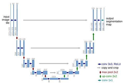
As illustrated in Figure 1, the U-Net network is distinguished by its architecture, which consists of three key components: an encoder, a decoder, and a bottleneck layer. The encoder is responsible for feature extraction and learning from the target object through four stages of convolutional and pooling operations, progressively decreasing the size of the feature maps. During the decoding process, the feature maps are upsampled to restore them to the original image size. Concurrently, the innovative skip connection algorithm integrates shallow and deep feature information. This architecture allows U-Net to effectively learn from small-scale datasets in medical imaging.
|
| Figure 1. U-Net network architecture diagram |
2.2 Swin-Unet network
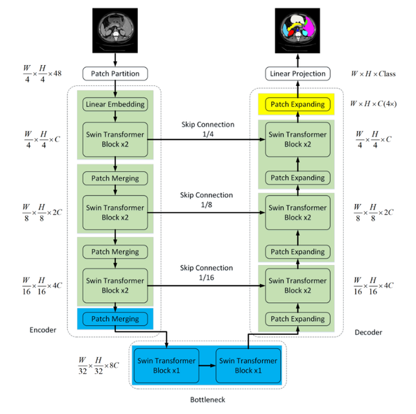
Within the domain of medical image segmentation, the demands for precision are exceedingly high. While CNN segmentation algorithms have achieved significant advancements in recent years, they still fall short of the stringent criteria required for medical applications. To address this gap, the Swin-Unet network was introduced, merging the capabilities of U-Net with the Swin Transformer. Figure 2 illustrates the comprehensive structure of this network.
Encoder Part: The Swin-Unet network significantly modifies the convolutional pooling operations of the original U-Net network, replacing them with multiple basic unit blocks from the Swin Transformer network. Each unit block in the network is capable of computing self-attention through local and global perception layers, allowing it to capture image features at various scales.
Decoder Component: Comparable to the U-Net architecture, Swin-Unet incorporates skip connections during upsampling, reinstating the reduced feature maps to the original image dimensions. However, the key distinction lies in replacing conventional convolutional operations with Swin Transformer blocks for feature learning.
|
| Figure 2. Swin-UNet network architecture diagram |
3. Improved U-Net network
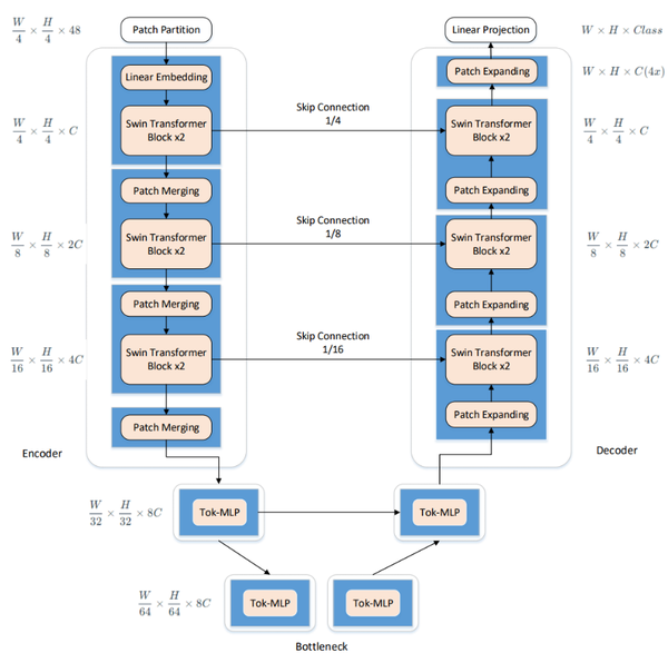
The enhanced U-Net network presented in this paper intelligently integrates the traditional U-Net with elements from Swin-Unet. It utilizes the U-Net structure as the backbone, replacing its convolutional units with Swin Transformer Blocks derived from Swin-Unet. This integration allows for the effective combination of global and local contextual information, thus enhancing segmentation accuracy and robust generalization. Additionally, multi-layer perceptrons are employed at lower levels to model complex features, which significantly reduces both computational complexity and the number of parameters, while still maintaining high segmentation accuracy. The comprehensive framework of this model is showed in Figure 3.
|
| Figure 3. Schematic of the improved U-Net network structure |
3.1 Improved network composition
3.1.1 Encoder
In the encoder, traditional convolutional operations, typical in the U-Net network, are replaced with Swin Transformer Blocks from the Swin-Unet architecture to enhance feature learning. Following each operation, a patch merging layer is utilized for downsampling, reducing the size and channel count of the feature maps. Downsampling takes place at a factor of 2 during each operation, wherein elements are selected at fixed positional intervals along both row and column directions before being concatenated.
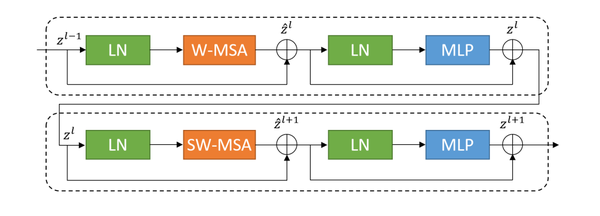
Distinguishing itself from traditional modules, the concept of a movable window is introduced into the improved network units. As shown in Figure 4, the structure diagram of a basic unit block is presented.
|
| Figure 4. Schema of swin transfomer block |
Each unit block within the network is configured to encompass layer normalization (LN), a multi-head self-attention mechanism (MSA), a residual connection, and two multilayer perceptrons (MLP). The block incorporates two types of attention mechanisms: a window-based multi-head self-attention mechanism (W-MSA) and a shifted window-based multi-head self-attention mechanism (SW-MSA) [12]. This design facilitates the employment of continuous unit blocks that utilize a movable window concept, enhancing the flexibility and effectiveness of the attention mechanisms in capturing varying spatial features.
|
|
(1) |
|
|
(2) |
|
|
(3) |
|
|
(4) |
In Eqs. (1) and (2), and represent the outputs of the (SW-MSA) module and the MLP module of the first block, respectively. The computational approach for self-attention is as follows:
|
|
(5) |
In Eq. (5), , , represent the query, key, and value, respectively. and denote the number of patches in the window and the dimension of the query or key, respectively. The value is derived from the bias matrix .
3.1.2 Shifted MLP
During the shifted MLP stage, before tokenization, the first operation performed is to shift the axes of the convolutional feature channels, aiding the multilayer perceptrons in focusing solely on the positional features of the convolutional features. To introduce more locality into the originally entirely global model, a window-based attention mechanism is employed at this stage, enabling the model to better integrate both global and local feature information. As illustrated in Figure 5, the shifted MLP schematic depicts features moving across width and height within two blocks, dividing features into different partitions and shifting their positions along the specified axes.

|
| Figure 5. Diagram of the shifted MLP (multilayer perceptron) |
3.1.3 Tokenized MLP stage
In the tokenized MLP stage, features undergo an initial transformation and projection onto tokens, where the channel count is adapted to align with the number of tokens. This step ensures proper correspondence between feature dimensions and the token structure. Subsequently, the tokens are forwarded to the shifted MLP for cross-width movement. The entire process employs depth-wise separable convolution (DWConv) for the following reasons:
1. Depth-wise separable convolution is advantageous for encoding positional information of features. Experimental results indicate that convolutional layers in MLPs are sufficient for encoding positional information and outperform standard positional encoding in practical performance.
2. DWConv has fewer parameters. In the tokenized MLP stage, the features are initially transformed and projected onto tokens, with the channel count adjusted to match the number of tokens.
The computational process of the tokenized MLP stage module involves:
|
|
(6) |
|
|
(7) |
|
|
(8) |
|
|
(9) |
3.1.4 Decoder
The decoder has a symmetric structure to the encoder, both composed of Swin Transformer block unit modules. The key distinction involves the use of patch expansion operations in the decoder, which essentially serve as the inverse of patch merging operations. This reversal process is critical for reconstructing the image from compressed features to its original dimensionality during the decoding phase. It performs upsampling operations on the features extracted by the decoder and reassembles the feature maps into higher-resolution ones.
3.1.5 Skip connection
Similar to most U-shaped network structures, skip connection operations fuse the feature information of downsampling and upsampling, effectively reducing information loss during downsampling to achieve better thyroid nodule segmentation.
4. Experiment and results
4.1 Experimental dataset
The thyroid nodule ultrasound scan images used in this study are sourced from the publicly available TN3K (thyroid nodule 3 thousand) dataset (Gong et al., 2021), which includes 3493 ultrasound images with pixel labels. The dataset comprises high-quality nodule mask annotations from various devices and views.
4.2 Experimental design
The experimental setup includes the following parameters: image dimensions are uniformly adjusted to , with an initial learning rate set at 0.0005, and a batch size of 8. The Adam optimizer is employed for model optimization. The models undergo training across over a span of 100 epochs.
The loss function treats each pixel as an independent binary classification problem, calculating the loss for each pixel. It offers good and stable focus on individual pixels. While the loss function demonstrates excellent experimental performance for small target objects, maintaining stable training results is challenging. Based on the above studies, this paper aims to balance stability and accuracy in thyroid nodule segmentation training. Therefore, the is utilized during training, combining the advantages of both loss functions to achieve better experimental results.
The (Binary Cross-Entropy) loss function is defined as follows:
|
|
(10) |
In Eq. (10), represents the initial thyroid nodule image, the true labels, and the corresponding predicted labels.
The loss function is defined as:
|
|
(11) |
In Eq. (11), represents a smoothing coefficient, which prevents situations like zero denominators. The computation of is as follows:
|
|
(12) |
5. Results and discussion
5.1 Evaluation metrics
The evaluation metrics employed include the coefficient, precision (), recall (), and -score. The coefficient measures the similarity between sets. Values for the loss function fall within the range of 0 to 1, with higher values denoting improved segmentation performance achieved by the model. Precision, recall, and -score provide additional insights into the accuracy and reliability of the segmentation.
The formula for calculating the coefficient is as follows:
|
|
(13) |
In Eq. (13), and represent the actual and predicted areas of the image, respectively.
The formulas for calculating precision (), recall (), and the -score are as follows:
|
|
(14) |
|
|
(15) |
|
|
(16) |
5.2 Results and analysis
5.2.1 Comparing the training effects of different loss functions
The initial set of experiments aims to assess the training effects of the enhanced network model proposed in this paper, employing , , and loss functions.
As shown in Table 1, based on the data analysis provided in the table above, it is apparent that for the enhanced neural network proposed in this paper, when trained using the loss function, the score is 0.9016, which represents the lowest score among the evaluated functions. However, when the model is trained using the loss function, a slight improvement is observed compared to utilizing the function, with the score increasing to 0.9031.
When combining the loss function with the loss function for training thyroid nodule ultrasound images, experimental results show that compared to using each loss function individually, the combination of both yields the highest coefficient, precision, and score, reaching 0.9062, 0.9153, and 0.9062, respectively. The results suggest that the enhanced U-Net network proposed in this paper demonstrates superior performance in balancing stability and segmentation effectiveness when utilizing the loss function.
| Loss Function | ||||
|---|---|---|---|---|
| 0.9016 | 0.9142 | 0.8959 | 0.9016 | |
| 0.9031 | 0.9074 | 0.9044 | 0.9031 | |
| 0.9062 | 0.9153 | 0.9023 | 0.9062 |
5.2.2 Comparison of segmentation performance of different networks
To further assess the effectiveness of the enhanced model presented in the study, the same dataset is used to train three distinct network models: U-Net, Swin-Unet, and the enhanced model. Subsequently, the segmentation accuracy is evaluated.
Based on Table 2, the score of the Swin-Unet network reaches 0.7322, which is the lowest among the evaluated networks. The U-Net network achieves a score of 0.8971, presenting a notable improvement of 22.52% compared to Swin-Unet. After optimization, the enhanced neural network proposed in this paper achieves the highest value of 0.9062 and the highest accuracy of 0.9153. Compared to Swin-Unet, it demonstrates a substantial enhancement of 23.76% and 23.67%, respectively. Furthermore, compared to U-Net, it also showcases improvements of 1.01% and 2.69%, respectively. In summary, the enhanced network proposed in this paper exhibits the most superior segmentation performance.
| Network | ||||
|---|---|---|---|---|
| Swin-Unet | 0.7322 | 0.7401 | 0.7524 | 0.7322 |
| U-Net | 0.8971 | 0.8913 | 0.9106 | 0.8971 |
| Improved U-Net | 0.9062 | 0.9153 | 0.9023 | 0.9062 |
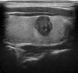
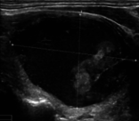
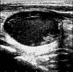
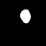
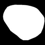
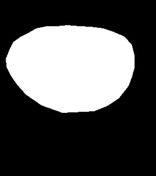
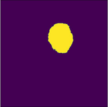
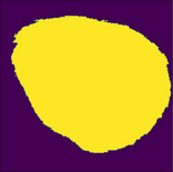
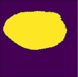
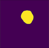
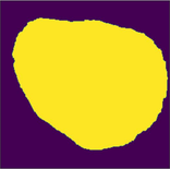
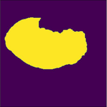
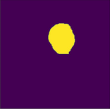
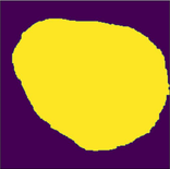
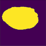
Figure 6 illustrates the segmentation outcomes attained with different neural networks using the same dataset. The enhanced U-Net network proposed in this study is evaluated alongside expert gold standards, Swin-Unet, U-Net, and other well-known network models. The segmentation results from the Swin-Unet network show jagged edges and less smooth nodule edge segmentation, leading to suboptimal outcomes. In the case of U-Net, there are evident under-segmentations with significant discrepancies in the segmented area of some nodules, resulting in inaccurate segmentation results. However, the use of the improved U-Net network introduced in this research produces smoother edges of the segmented thyroid nodules, and the edge contours more closely align with those of the expert gold standard. Moreover, the errors in shape and segmented area are smaller compared to those seen with U-Net and Swin-Unet. The findings suggest that the improved U-Net network provides superior performance in thyroid nodule segmentation.
This paper presents a method that improves upon the original U-Net network by replacing the standard convolutional blocks in the U-Net architecture with Swin Transformer blocks. This modification introduces local-to-global self-attention mechanisms in the encoder, significantly improving the model’s ability to generalize robustly. Additionally, a tokenized multilayer perceptron module is integrated to effectively model features using multilayer perceptrons. Following downsampling in the encoder, features are efficiently tokenized and projected. Through the adoption of a parameter-efficient design, the model attains an optimal equilibrium between segmentation accuracy and computational efficiency.
6. Conclusions
This study provides an enhanced neural network derived from U-Net for the segmentation of thyroid nodule ultrasound images. The following enhancements are incorporated into the U-Net network:
1. Integration of unit modules from Swin Transformer into the model encoder for feature learning, enabling a self-attention mechanism from local to global.
2. Employing multilayer perceptrons (MLPs) at the lower levels for feature modeling, while considering the impact of model dimensions on parameter count and computational complexity in the overall design. This design choice reduces parameter count and improves segmentation speed and accuracy.
3. Combining the advantages of both and loss functions by using the loss function, which balances stability and segmentation accuracy, further enhancing the model’s performance.
Experimental findings suggest that the enhanced network model proposed in this study attains superior segmentation accuracy metrics. Specifically, it achieves a coefficient of 0.9062, a precision rate of 0.9153, an average recall of 0.9023, and an average score of 0.9.
References
[1] Guth S., Theune U., Aberle J., Galach A., Bamberger C.M. Very high prevalence of thyroid nodules detected by high frequency (13 MHz) ultrasound examination. Eur. J. Clin. Invest., 39:699–706, 2009.
[2] Haugen B.R., Alexander E.K., Bible K.C., et al. 2015 American Thyroid Association management guidelines for adult patients with thyroid nodules and differentiated thyroid cancer: the American Thyroid Association Guidelines Task Force on thyroid nodules and differentiated thyroid cancer. Thyroid, 26:1–133, 2016.
[3] Ronneberger O., Fischer P., Brox T. U-net: Convolutional networks for biomedical image segmentation. International Conference on Medical Image Computing and Computer-Assisted Intervention, Munich, Germany, pp. 234-241, 2015.
[4] Ma X., Sun B., Liu W., et al. AMSeg: A novel adversarial architecture based multi-scale fusion framework for thyroid nodule segmentation. IEEE Access, 11:72911-72924, 2023.
[5] Hu Y., Qin P., Zeng J., et al. Ultrasound thyroid segmentation network based on feature fusion and dynamic multi-scale dilated convolution. Journal of Computer Applications, 41(3):891-897, 2021.
[6] Sun J., Li C., Lu Z., et al. TNSNet: Thyroid nodule segmentation in ultrasound imaging using soft shape supervision. Computer Methods and Programs in Biomedicine, 215, 106600, 2022.
[7] Chu C., Zheng J., Zhou Y. Ultrasonic thyroid nodule detection method based on U-Net network. Computer Methods and Programs in Biomedicine, 199:105906-105912, 2021.
[8] Oktay O., Schlemper J., Folgoc L.L., et al. Attention u-net: Learning where to look for the pancreas. arXiv preprint arXiv:1804.03999, 2018.
[9] Zhou Z., Rahman Siddiquee M.M., Tajbakhsh N., et al. Unet++: A nested u-net architecture for medical image segmentation. In: Stoyanov, D., et al. Deep Learning in Medical Image Analysis and Multimodal Learning for Clinical Decision Support, DLMIA ML-CDS 2018 2018. Lecture Notes in Computer Science, vol. 11045, Springer, Cham., 3-11, 2018.
[10] Chen L.C., Zhu Y., Papandreou G., et al. Encoder-decoder with atrous separable convolution for semantic image segmentation. Proceedings of the European conference on computer vision (ECCV), Munich, Germany, 801-818, 2018.
[11] Badrinarayanan V., Kendall A., Cipolla R. Segnet: A deep convolutional encoder-decoder architecture for image segmentation. IEEE Transactions on Pattern Analysis & Machine Intelligence, 39(12):2481-2495, 2017.
[12] Dan Y., Jin W., Wang Z., et al. Optimization of U-shaped pure transformer medical image segmentation network. PeerJ Computer Science, 9, 1515, 2023.Document information
Published on 06/06/24
Accepted on 23/05/24
Submitted on 20/05/24
Volume 40, Issue 2, 2024
DOI: 10.23967/j.rimni.2024.05.012
Licence: CC BY-NC-SA license
