| Line 87: | Line 87: | ||
where <math display="inline">g_t </math> is the candidate state obtained through a nonlinear function, as shown in Eq.(4) | where <math display="inline">g_t </math> is the candidate state obtained through a nonlinear function, as shown in Eq.(4) | ||
| − | + | {| class="formulaSCP" style="width: 100%; text-align: left;" | |
| − | + | |- | |
| + | | | ||
| + | {| style="text-align: center; margin:auto;width: 100%;" | ||
| + | |- | ||
| + | | style="text-align: center;" | <math>g_t=\tanh\left(W_{ig}x_t+b_{ig}+W_{hg}h_{t-1}+b_{hg}\right)</math> | ||
| + | |} | ||
| + | | style="width: 5px;text-align: right;white-space: nowrap;" |(4) | ||
| + | |} | ||
| − | + | where <math display="inline">f_t \in [0,1]</math> is the forget gate, which controls how much information from the previous internal state <math>c_{t-1}</math> should be forgotten, as shown in Eq.(5) | |
| − | + | {| class="formulaSCP" style="width: 100%; text-align: left;" | |
| − | + | |- | |
| + | | | ||
| + | {| style="text-align: center; margin:auto;width: 100%;" | ||
| + | |- | ||
| + | | style="text-align: center;" | <math>i_t=\sigma \left(W_{ii}x_t+b_{ii}+W_{hi}h_{t-1}+b_{hi}\right)</math> | ||
| + | |} | ||
| + | | style="width: 5px;text-align: right;white-space: nowrap;" |(5) | ||
| + | |} | ||
| − | + | where <math display="inline">i_t \in [0,1]</math> represents the input gate, which controls how much information the candidate state <math display="inline">g_t </math> should store at the current time step, as shown in Eq.(6) | |
| − | + | {| class="formulaSCP" style="width: 100%; text-align: left;" | |
| − | + | |- | |
| + | | | ||
| + | {| style="text-align: center; margin:auto;width: 100%;" | ||
| + | |- | ||
| + | | style="text-align: center;" | <math>f_t=\sigma (W_{if}x_t+b_{if}+W_{hf}h_{t-1}+b_{hf})</math> | ||
| + | |} | ||
| + | | style="width: 5px;text-align: right;white-space: nowrap;" |(6) | ||
| + | |} | ||
| − | + | where <math display="inline">o_t \in [0,1]</math> represents the output gate, which controls how much information from the current internal state <math display="inline">c_t </math> is output to the external state <math display="inline">h_t </math>, as shown in Eq.(7) | |
| − | + | {| class="formulaSCP" style="width: 100%; text-align: left;" | |
| − | + | |- | |
| + | | | ||
| + | {| style="text-align: center; margin:auto;width: 100%;" | ||
| + | |- | ||
| + | | style="text-align: center;" | <math>o_t=\sigma \left(W_{io}x_t+b_{io}+W_{ho}h_{t-1}+b_{ho}\right)</math> | ||
| + | |} | ||
| + | | style="width: 5px;text-align: right;white-space: nowrap;" |(7) | ||
| + | |} | ||
| − | + | where <math display="inline">x_t</math> is the input at the current time step, and <math>h_{t-1}</math> is the external state at the previous time step; <math display="inline">w_{ii}</math>, <math display="inline">b_{ii}</math>, <math display="inline">w_{if}</math>, <math display="inline">b_{if}</math>, <math display="inline">w_{io}</math>, <math display="inline">b_{io}</math>, <math display="inline">w_{ig}</math>, <math display="inline">b_{ig}</math> are parameter matrices for the linear transformation of input <math display="inline">x_t</math>; <math display="inline">w_{hi}</math>, <math display="inline">b_{hi}</math>, <math display="inline">w_{hf}</math>, <math display="inline">b_{hf}</math>, <math display="inline">w_{ho}</math>, <math display="inline">b_{ho}</math>, <math display="inline">w_{hg}</math>, <math display="inline">b_{hg}</math> are the parameter matrices for the linear transformation of <math>h_{t-1}</math>; <math display="inline">\sigma (x)</math> is the activation function, whose range is <math>(0,1)</math>, and is defined by Eq.(8) | |
| + | |||
| + | {| class="formulaSCP" style="width: 100%; text-align: left;" | ||
| + | |- | ||
| + | | | ||
| + | {| style="text-align: center; margin:auto;width: 100%;" | ||
| + | |- | ||
| + | | style="text-align: center;" | <math>\sigma \left(x\right)=\frac{1}{1+exp\left(-x\right)}</math> | ||
| + | |} | ||
| + | | style="width: 5px;text-align: right;white-space: nowrap;" |(8) | ||
| + | |} | ||
| − | |||
| − | |||
The computation process of LSTM neural network is as follows: | The computation process of LSTM neural network is as follows: | ||
| − | (1) Calculate three gates and a candidate state | + | (1) Calculate three gates and a candidate state <math display="inline">g_t </math> using the current input <math display="inline">x_t</math> and the previous external state <math>h_{t-1}</math>. |
| − | (2) Update the memory cell | + | (2) Update the memory cell <math display="inline">c_t </math> through the forget gate <math display="inline">f_t </math> and the input gate <math display="inline">o_t </math>. |
| − | (3) Use the output gate | + | (3) Use the output gate <math display="inline">o_t </math> to pass the information from the internal state to the external state <math display="inline">h_t </math>. |
==2.2 PSO (Particle Swarm Optimization)== | ==2.2 PSO (Particle Swarm Optimization)== | ||
Revision as of 13:40, 12 January 2024
Abstract
Based on the construction data of Fuzhou Metro Line 4 in Fujian Province, China, this paper proposes a soil pressure prediction model that combines Long Short-Term Memory (LSTM) and Particle Swarm Optimization (PSO). The values of Mean Absolute Error, Mean Squared Error, and Coefficient of Determination are 0.007MPa, 0.007%, and 0.93, respectively, indicating an improvement in accuracy.Wang-Mendel algorithm is used to establish fuzzy rules. The Mean Absolute Error and Mean Squared Error of the rotating speed of the screw machine are 0.065rpm and 1.528%, and the Coefficient of Determination is 0.82. The calculation accuracy of this algorithm is high.A set of knob intelligent control device is developed.The Mean Absolute Error and Mean Squared Error of 0.015rpm and 0.392%, respectively, and the Coefficient of Determination of 0.95, indicating a small execution error of the device. This paper provides a new and effective method for the control of EPB shield pressure.
Keywords: EPB, soil pressure prediction, LSTM, PSO
1. Introduction
EPB uses dynamic balance control of water and soil pressure in front of the excavation face to avoid surface deformation. Soil pressure control involves multi-field coupling of multiple subsystems, such as the cutterhead system, propulsion system, and screw conveyor system, as well as the comprehensive effects of multiple factors such as excavation parameters and muck properties. Therefore, establishing a soil pressure control model is one of the key challenges in shield tunneling technology.Currently, the control of soil pressure in shield tunneling is generally achieved through two approaches: the establishment of a mechanism model based on mathematical and physical relationships or the use of intelligent methods such as neural networks based on on-site data. With an accurate model, it is possible to make correct predictions of future states based on past and current conditions and then optimize and control controllable variables to achieve effective control of soil pressure.
Previous studies have conducted extensive research on earth pressure balance.Hu et al. used electro-hydraulic proportional control technology to control the propulsion speed or screw machine speed in real-time on a simulation experimental platform, demonstrating that controlling the screw machine speed can achieve control of soil pressure. Based on this, they further used self-tuning PID to regulate the screw conveyor speed to achieve control of soil pressure [1]. Wang and Fu derived three basic equations for EPB shield based on model test results, and then obtained two total balance equations for EPB shield, establishing a mathematical model for EPB shield excavation [2]. Wang et al. proposed a soil pressure balance control system based on the feedback of advance speed and soil pressure, building upon previous mechanism models [3]. In recent years, neural networks have been widely used in soil pressure prediction and shield tunneling. Yeh pioneered the use of neural networks in the control of soil pressure by using a backpropagation neural network to establish a control model with the current soil pressure, advancing speed, screw conveyor speed, next moment advancing speed, next moment screw conveyor speed as inputs and next moment soil pressure as output [4]. Wei et al. combined Monte Carlo method and BP neural network model to predict the TBM's advancing speed [5]. Gao et al. used three types of recurrent neural networks (RNNs) to process real-time prediction data based on on-site TBM operating parameters, and showed that the three proposed RNN-based predictors outperformed classical regression models [6]. Liu et al. developed a long short-term memory (LSTM) network based on a global attention mechanism to predict the lithology of the excavation face [7]. Cachim and Bezuijen used a multi-layer feedforward artificial neural network to predict the cutterhead torque of an EPB-TBM, and used a time-series neural network to predict the torque as a function of the measured torque and injected foam volume at the previous time step [8]. Song et al. proposed a time series segmentation method based on fuzzy c-means clustering for TBM time series data [9]. Shi et al. proposed a new clustering algorithm based on support vector regression and fuzzy c-means algorithm (SVR-FCM) [10]. Sun et al. developed a prediction model based on integrated heterogeneous in-situ data using data-driven techniques. This method was applied in the field of non-homogeneous tunnel boring machine, which not only accurately predicted the dynamic characteristics of the load, but also accurately estimated the statistical characteristics of the load [11].
Some scholars have made research on control and particle swarm optimization. Wen et al. proposed a soil discharge prediction method based on an adaptive adjustment strategy and parameters to achieve optimal regression. The study analyzed the factors affecting soil flow data models using actual engineering data and found that the screw conveyor speed and total thrust were the main factors affecting the soil flow rate [12]. Liu et al. proposed an optimized control method for earth pressure based on ADHDP, which realized the online autonomous learning and adaptive control of shield tunneling chamber pressure [13]. Zhang used artificial experience to train and learn the membership functions and fuzzy rule parameters of a fuzzy system using neural networks. They established an ANFIS model for predicting the soil pressure in the shield tunneling machine and used genetic algorithms for optimizing control [14]. Zhu used a fuzzy PID control algorithm to control the factors that affect the earth pressure, and verified the correctness of the algorithm through experimental simulation [15]. Li and Gong proposed a model predictive control (MPC) system for predicting and controlling mud pressure balance during construction. The system consists of a diagonal recurrent neural network (DRNN), an optimizer that generates optimal air pressure and slurry level based on multi-step prediction, and an evolved particle swarm optimization (EPSO) algorithm. It can effectively adjust the mud circulation and air pressure maintenance system according to geological conditions [16]. Li and Li used a BP neural network for prediction and adopted the PSO algorithm to calculate the balanced control of the screw conveyor speed required for the next moment[17]. Zhang et al. proposed a method for controlling the shield tunneling machine's earth pressure using a fuzzy PID control approach based on a mechanistic model. The method was compared with the traditional PID control method, and the results showed that the proposed approach was more effective [18]. Yang developed a PSO-BP model for predicting the soil pressure in the tunnel and obtained the relationship between the predicted soil pressure and the screw conveyor speed using polynomial fitting to achieve control of soil pressure [19].
After reviewing the research status above, it was found that the input parameters considered in the mechanism control model are limited, and it is difficult to obtain some parameters such as the screw conveyor excavation efficiency and the tangential modulus of deformation of the spoil. In intelligent control models such as neural networks, after the pressure prediction model is obtained, the corresponding screw conveyor speed needs to be calculated using algorithms such as PSO and genetic algorithms, which is time-consuming. In order to facilitate engineering application, this paper will establish a PSO-LSTM deep neural network prediction model, use the WM algorithm to establish fuzzy rules for easy calculation, and develop an intelligent control device. The feasibility of the device will be verified through actual engineering data.
2. Theoretical background
2.1 LSTM neural network
In many studies that use neural networks, it is necessary to deal with sequential data and utilize its historical information. Therefore, it is necessary to enable neural networks to have memory function. The long short-term memory (LSTM) network is selected, and its structure is shown in Figure 1.
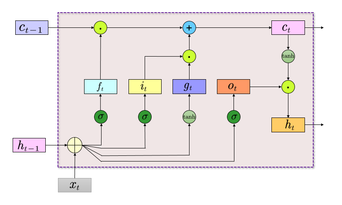
|
| Figure 1. LSTM network structure |
LSTM network introduces an internal state specifically for the linear recurrent information transfer, as shown in Eq.(1). At the same time, it transfers the non-linear output information to the external state of the hidden layer, as shown in Eq.(2):
|
|
(1) |
|
|
(2) |
In Eqs.(1) and (2), represents, at each time step , the internal state stores the historical information from the beginning up to the current time step; ⊙denotes element-wise multiplication of vectors; is the memory cell from the previous time step; is both the current time step 's output of the hidden layer and the input of the hidden layer for the next time step ; is the activation function, defined by Eq.(3), with a range of ;
|
|
(3) |
where is the candidate state obtained through a nonlinear function, as shown in Eq.(4)
|
|
(4) |
where is the forget gate, which controls how much information from the previous internal state should be forgotten, as shown in Eq.(5)
|
|
(5) |
where represents the input gate, which controls how much information the candidate state should store at the current time step, as shown in Eq.(6)
|
|
(6) |
where represents the output gate, which controls how much information from the current internal state is output to the external state , as shown in Eq.(7)
|
|
(7) |
where is the input at the current time step, and is the external state at the previous time step; , , , , , , , are parameter matrices for the linear transformation of input ; , , , , , , , are the parameter matrices for the linear transformation of ; is the activation function, whose range is , and is defined by Eq.(8)
|
|
(8) |
The computation process of LSTM neural network is as follows:
(1) Calculate three gates and a candidate state using the current input and the previous external state .
(2) Update the memory cell through the forget gate and the input gate .
(3) Use the output gate to pass the information from the internal state to the external state .
2.2 PSO (Particle Swarm Optimization)
Particle Swarm Optimization (PSO) is mainly inspired by the collective behavior of bird flocking and the cognitive mechanism of humans.Assuming the position of particle i randomly placed in the search space is xi=(x1,x2,···,xid,···,xin)and its velocity is vi=(vi1,vi2,···,vid,···,vin), then the individual best value of the particle based on the fitness function is Pi=(Pi1,Pi2,···,Pid,···,Pin), and the global best value of the swarm is Pgi=(Pg1,Pg2,···,Pgd,···,Pgn). The evolution equations for the particle swarm algorithm are given by Eq. 9 and 10.
In the equation, ωis the weight coefficient: d = 1, 2, 3... N; k is the current iteration number; c1c2,r1r2 are non-negative constants randomly distributed in [0,1]; to avoid large-scale blind search, the range of particle positions and velocities are limited to[-Xmax,Xmax] and [-Vmax,Vmax], respectively.
In this paper, PSO algorithm is mainly used to optimize the hyperparameters in the soil pressure prediction model. Therefore, the error between the predicted values obtained by the prediction model and the actual values is used as a reference value for the fitness function, and the optimization goal is to find the best combination of hyperparameters for the deep neural network. The relationship between the model to be optimized and the optimization goal can be expressed as Eq.11:
Where ytest is the predicted result of the model; ytrue is the actual value; Ntest is the number of test samples selected.
The process of optimizing the prediction model using PSO can be summarized as follows:
(1) Initialize PSO parameters and set initial values for hyperparameters of the deep neural network prediction model. Calculate the initial position for each particle, denoted as PBest, and set the best value in PBest as the global optimal value gBest.
(2) Calculate the fitness value of the prediction model by using the error between the predicted values obtained by each particle and the actual values, and record the current particle position and corresponding fitness function value.
(3) Compare the fitness value of the particle with the best fitness value it has reached, update the particle's velocity and position, and optimize.
(4) If the number of iterations is not completed, return to step 2 to continue the operation, and finally obtain the globally optimal hyperparameter combination.
2.3Wang-Mendel algorithm
The Wang-Mendel (WM) method proposed by Wang and Mendel can effectively generate fuzzy rules from sample data [20]. This method partitions the input space into fuzzy regions and then uses a lookup table to extract rules for each fuzzy subspace. The WM method does not require repeated learning and can use a large amount of input-output data to obtain a complete fuzzy rule base that covers the entire input domain [21]. The WM method has become a classic method for fuzzy rule generation and has been widely used in various applications [22].
Therefore, in this study, the WM (Wang-Mendel) algorithm was used to establish a fuzzy rule base, which mainly includes three steps: rule extraction, rule merging, and rule inference [21].
Rule extraction refers to extracting fuzzy rules from input factor data. Firstly, the input factors xj should be divided into mj fuzzy subsets. In this paper, the input data is in the form of n inputs and one output, which can be expressed as:(x(I),y),I=1,2,…,n.Where x(I)∈Rn represents the input factors and y∈R represents the output factor. The input factor data is fuzzified and divided into L fuzzy subspaces using the triangular membership function Eq.14 as shown in Eq.13. Then, one rule can be extracted from each of the K data points, as shown in Eq.12. In this way, K rules are obtained.
Where l=1,...,L; there are mn fuzzy sets {Albn|lb=1,…,mn} on the input domain of input factor xn. Albn represents the fuzzy set on input xb with index ld; Bl represents the fuzzy set on the output domain UBl(y)=u(y,yl c,σl).σ is the width of the fuzzy set, yc is the center point of the fuzzy set, defined by Eq.16 and 15, where y∈[yc-σ,yc+σ].l is the rule index corresponding to it in the rule base.L fuzzy sets correspond to L fuzzy rules. Then, the rules with the same premise conditions are merged, and the confidence degrees of the duplicate and conflicting rules are calculated. By comparing the confidence degrees, the rules with low confidence are removed. Suppose there are H groups of duplicate rules, each containing Nh rules. The weight of each rule is calculated using Eq.17. The larger the weight, the closer the rule is to the center of the fuzzy space. Then, Nh rules are merged into a single rule in the form of Eq.12, and the reliability of the rule is calculated using Eq.18. Finally, the reliable rules are selected and added to the rule base.
(17)3 Process and Analysis
3.1 Data Acquisition and Cleaning
The research data in this paper is based on the construction site of Subway Line 4 in Fuzhou City. Data is collected and saved to the database in real-time at intervals of one minute.
In the research process, the correct selection of factor data determines the correct match between the analysis object and the results. Due to the large number of excavation factor data generated by the shield machine during the excavation process, and the existence of missing values and outliers to some extent in each factor, it is necessary to clean the raw data to improve the quality of factor data.
The effectiveness of data cleaning directly affects the accuracy of subsequent data analysis and model predictions. Through investigation and monitoring of the construction site of Fuzhou Metro Line 4, based on traditional data preprocessing methods and fully considering factors such as the shield tunneling construction process, construction conditions, and the operator's habits, this article formulated the following five data cleaning principles:
(1) Based on detailed geological survey data, select shield tunneling data under the same geological conditions as the research object, excluding the influence of different geological conditions on the soil pressure caused by the shield machine.
(2) Due to the large amount of data, delete the real-time factor data corresponding to missing or abnormal values in each factor to ensure the correspondence between the data of each factor.
(3) Data corresponding to abnormal tunneling states such as stand-by, stoppage, cutterhead replacement, and mechanical failure are deleted to ensure that the data only includes those from normal tunneling processes of the shield machine.
(4) Data for monitoring factors such as horizontal deviation, front and rear mileage, mechanical and electrical parameters, and vertical deviation with values of 0 are removed.
(5) If the data of a certain factor is 0, the corresponding real-time data of other factors will be deleted to ensure the correspondence between each factor data.
After applying the above data cleaning principles, a total of 27 rings, 3525 sets of data, and 32 excavation factors were selected in the excavation factors data ranging from ring 407 to 434.
3.2 Spearman Correlation Analysis
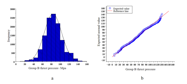
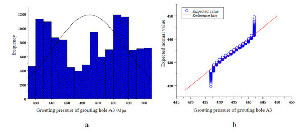
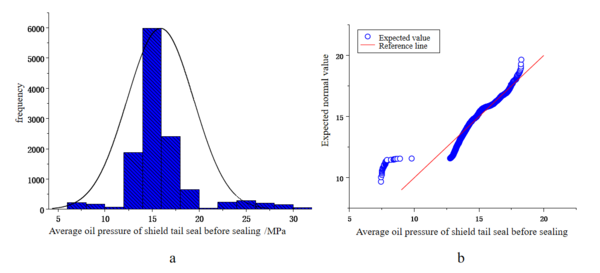
In this paper, to investigate whether there is a relationship between the shield tunneling factors and the earth pressure in the cutterhead chamber, as well as the degree of correlation, it is necessary to perform a correlation analysis.Two commonly used methods for correlation analysis are the Pearson correlation coefficient and the Spearman correlation coefficient. The Pearson correlation coefficient belongs to parametric statistical methods, while the Spearman correlation coefficient belongs to non-parametric statistical methods.Therefore, it is necessary to perform normality test on the 32 data factors obtained from the previous data cleaning. This article lists the histograms and Q-Q plots of the following three excavation factors, as shown in Figures 2 to 4.As shown in the figures, some factors follow normal distribution while others do not, indicating that the Spearman correlation coefficient should be chosen for analysis.
The Spearman correlation coefficient, also known as the rank correlation coefficient, is calculated using the following Eq.19:
In the Eq.,Ri andSi represent the rank order of the observed value i; R andS are the average rank orders of x and y, respectively; N is the total number of observed values.
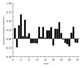
Apart from the factor of silo pressure, this study conducted correlation analysis between 31 other factors and silo pressure using SPSS. The results are shown in Table 1 and Figure 5.The value of the Spearman correlation coefficient r ranges from -1 to 1, where values between 0 and 1 indicate a positive correlation and values between -1 and 0 indicate a negative correlation. The absolute value of the correlation coefficient |r| represents the degree of correlation between the two factors, and the correlation strength can generally be judged and described using Table 2 [23].
| Factor number | Factor name | Spearman correlation coefficient r | degree of correlation |
| 1 | Advance speed(mm/min) | 0.297** | Weak |
| 2 | Cutter speed(r/min) | -0.239** | Weak |
| 3 | Cutter Torque(kn.m) | 0.378** | Weak |
| 4 | Total thrust(kn) | 0.683** | Strong |
| 5 | Group A propulsion pressure(MPa) | 0.07** | Unrelated |
| 6 | Group B propulsion pressure(MPa) | 0.532** | Moderate |
| 7 | Group C propulsion pressure(MPa) | 0.062** | Unrelated |
| 8 | Group D propulsion pressure(MPa) | 0.151** | Unrelated |
| 9 | Group A advance displacement(mm/m) | -0.125** | Unrelated |
| 10 | Group B advance displacement(mm/m) | -0.122** | Unrelated |
| 11 | Group C advance displacement(mm/m) | -0.122** | Unrelated |
| 12 | Group D advance displacement(mm/m) | -0.129** | Unrelated |
| 13 | Grouting hole A1 grouting pressure(kn/m2) | 0.33** | Weak |
| 14 | Grouting hole A2 grouting pressure(kn/m2) | 0.049** | Unrelated |
| 15 | Grouting hole A3 grouting pressure(kn/m2) | 0.33** | Weak |
| 16 | Grouting hole A4 grouting pressure(kn/m2) | 0.025** | Unrelated |
| 17 | screw machine pressure(MPa) | 0.232** | Weak |
| 18 | Screw machine torque(KN2m) | 0.232** | Weak |
| 19 | Screw speed(rpm) | 0.326** | Weak |
| 20 | Spiral machine oil temperature(℃) | -0.188** | Unrelated |
| 21 | The average oil pressure of the shield front and tail seals(MPa) | 0.278** | Weak |
| 22 | The average oil pressure of the shield tail seal of the sealed warehouse(MPa) | 0.274** | Weak |
| 23 | Average pressure of foam system(MPa) | 0.464** | Moderate |
| 24 | Foam Circuit Average Air Flow(L/min) | 0.16** | Unrelated |
| 25 | Foam Circuit Average Liquid Flow(L/min) | -0.021 | Unrelated |
| 26 | Articulation cylinder pressure(MPa) | -0.119** | Unrelated |
| 27 | Group A articulated cylinder stroke(mm) | -0.153** | Unrelated |
| 28 | Group B articulated cylinder stroke(mm) | -0.211** | Weak |
| 29 | Group C articulated cylinder stroke(mm) | 0.165** | Unrelated |
| 30 | Group D articulated cylinder stroke(mm) | 0.332** | Weak |
| 31 | Foam water real-time cumulative average(m3/h) | -0.104** | Unrelated |
- **.exhibits significant correlation at the 0.01 level (two-tailed)
| |r| | correlation coefficient |
| (0,0.2] | Extremely Weak Correlation
/Unrelated |
| (0.2,0.4] | Weak Correlation |
| (0.4,0.6] | Moderate Correlation |
| (0.6,0.8] | Strong Correlation |
| (0.8,1] | Extremely Strong Correlation |
The correlation between total thrust and soil pressure is strongly correlated. The average pressure of the foam system and the push pressure of group B have a moderate correlation. The correlation between cutterhead torque, advance speed, cutterhead speed, grouting hole A1 grouting pressure, grouting hole A3 grouting pressure, screw conveyor pressure, screw conveyor torque, screw conveyor speed, average oil pressure of the front shield tail seal, average oil pressure of the rear shield tail seal, the stroke of the hinge oil cylinder of group B and group D have a weak correlation with soil pressure. Other factors have a very weak correlation and can be considered to have no correlation with soil pressure.
Therefore, this study finally determined 15 excavation factors including total thrust, B-group advance pressure, foam system average pressure, cutterhead torque, advance speed, cutterhead speed, grouting hole A1 grouting pressure, grouting hole A3 grouting pressure, screw conveyor pressure, screw conveyor torque, screw conveyor speed, average oil pressure of shield tail sealing at front chamber, average oil pressure of shield tail sealing at rear chamber, B-group articulated oil cylinder stroke, and D-group articulated oil cylinder stroke as inputs for the neural network prediction model.
3.3 Evaluation Indicators
The evaluation indicators selected in this paper are mean absolute error (MAE), mean squared error (MSE), and coefficient of determination (R2).The mean absolute error (MAE) is used in this paper to reflect the error between the actual and predicted values, and its Eq. is shown in Eq.20. The mean squared error (MSE) is used to evaluate the degree of data variation, and the smaller the value, the better the predictive model's ability to accurately describe the data, as shown in Eq.21 [24].The coefficient of determination R2 is used to evaluate the goodness-of-fit of a regression model. The closer its value is to 1, the better the performance of the model, as shown in Eq.22.
In the Eq., n represents the sample size; ŷi represents the predicted value; yi represents the actual value; and ȳi represents the mean value.
3.4 Model training
This paper builds an LSTM deep neural network prediction model using PyTorch deep learning framework, based on mini-batch gradient descent method and further optimized by Adam algorithm. In order to improve the accuracy of the LSTM prediction model, PSO is used to optimize LSTM parameters, and a PSO-BP prediction model is constructed using the classical BP neural network for comparison.The loss function of the prediction model is the root mean square error (RMSE) loss function. The training process is iteratively trained using the training set, and the prediction results are compared and analyzed using the test set. The hyperparameters of the four comparative models are tuned by parameter tuning, as shown in Table 3.
| Model parameters | learning_rate | lstm_layers | hidden_size | batch_size |
| LSTM | 0.001 | 3 | 52 | 612 |
| BP | 0.001 | 2 | 62 | 640 |
| PSO-LSTM | 0.005 | 3 | 46 | 1024 |
| PSO-BP | 0.001 | 3 | 48 | 820 |
| test group | MAE(MPa) | MSE(%) | R2 |
| PSO-BP | 0.010 | 0.018 | 0.84 |
| PSO-LSTM | 0.007 | 0.007 | 0.93 |
| LSTM | 0.011 | 0.015 | 0.87 |
| BP | 0.015 | 0.028 | 0.75 |
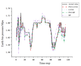
According to Figure 6 and Table 4, it can be seen that compared to the BP prediction model, the LSTM prediction model has reduced MAE from 0.015 MPa to 0.011 MPa by 26.7%, reduced MSE from 0.028% to 0.015% by 46.4%, and increased the absolute coefficient R2 from 0.75 to 0.87 by 16%. It can be seen that the LSTM prediction model is better than the BP prediction model in predicting the pressure of the soil bin.Compared with PSO-BP, PSO-LSTM reduced MAE from 0.010 MPa to 0.007 MPa, a decrease of 30%, reduced MSE from 0.018% to 0.007%, a decrease of 61.1%, and increased R2 from 0.84 to 0.93, an improvement of 10.7%. It can be seen that PSO-optimized LSTM prediction model performs better than PSO-optimized BP prediction model in predicting the pressure in the soil bin.Compared with the LSTM prediction model, the PSO-optimized model has reduced MAE from 0.011 MPa to 0.007 MPa, a decrease of 36.4%, MSE from 0.015% to 0.007%, a decrease of 53.3%, and R2 from 0.87 to 0.93, an increase of 6.9%, indicating that using PSO to optimize the LSTM prediction model can improve its prediction accuracy.
3.5 Fuzzy control
In order to achieve the application of intelligent control of shield machines in practical engineering, this paper needs to obtain the corresponding relationship between the soil pressure and the screw machine speed. As the six factors of advancing speed, cutterhead speed, total thrust, cutterhead torque, screw machine speed, and soil pressure can be obtained from the monitoring room of a shield machine, historical data of these six factors from ring 407 to 433 were selected as the training set, and the data from ring 434 was used as the test set to construct a 5-input single-output fuzzy control rule.
The maximum and minimum values of each factor are taken as the domain range, and the triangular membership function is used to automatically partition the fuzzy set based on the specified number of partition intervals for each factor. The data is then fuzzified, and the membership degree of each data point on the fuzzy set is calculated. The highest membership degree value is selected as the basis for a fuzzy rule. Due to the large number of repeated rules in these rules, their confidence levels are calculated separately and filtered to establish a fuzzy rule base.
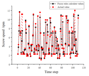
The predicted value of the 434th ring shield pressure obtained by the LSTM prediction model, together with the real-time read push speed, cutterhead speed, total thrust, and cutterhead torque that can be obtained from the shield machine monitoring room, are used as inputs to the fuzzy rules. The corresponding target value of the screw conveyor speed is obtained, as shown in Figure 7.
| Evaluation index | MAE(rpm) | MSE(%) | R2 |
| Fuzzy rule calculation value | 0.065 | 1.528 | 0.82 |
According to Table 5, the errors between the extracted fuzzy rules for screw machine speed and the actual values, obtained through the WM algorithm from historical data, are 0.065rpm for MAE, 1.528% for MSE, and 0.82 for absolute coefficient R2, indicating that the accuracy of the fuzzy rule base established by the algorithm is relatively high and basically meets the requirements.
3.6 intelligent control device
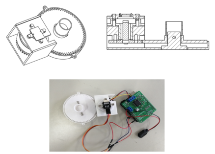
To achieve precise control of the screw conveyor, it is essentially precise control of the drive motor. Based on the actual situation of the Fuzhou Metro Line 4 shield machine control room, this paper uses an Arduino main control board, Simple FOC to drive a BLDC brushless DC motor, and an AS5600 magnetic encoder as the motor's position sensor to create an intelligent control device for the shield screw machine control knob, as shown in Figure 8.
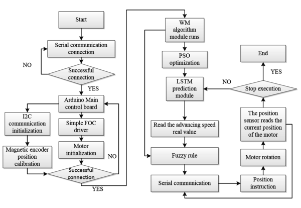
The working principle of the intelligent control device for the shield spiral conveyor is as follows: When the PC sends a position target command to the Arduino main control board through USB serial communication, the Simple FOC drives the BLDC brushless DC motor to start. The motor gear fixed on the top of the BLDC brushless DC motor rotates, and through the gear meshing with the knob gear, the motor torque is transmitted to the knob gear, thereby driving the speed knob of the spiral conveyor fixed by screws under the knob gear. The AS5600 magnetic sensor obtains the position data of the BLDC brushless DC motor rotation by fixing a radial magnet on the top of the cylindrical center of the motor gear, feeds it back to the Arduino main control board through I2C and transmits it to the PC through USB serial communication. The brushless DC motor stops rotating when it reaches the target position.
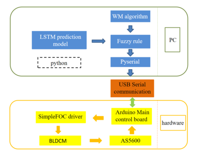
The intelligent control device established in this article mainly includes two parts: hardware and software. The key to establishing the overall control program is to realize the communication between Python and Arduino microcontroller. The structure of the overall control program established in this article is shown in Figure 9, and the control flow of the overall program is shown in Figure 10.
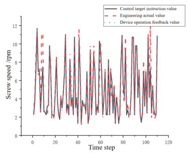
The performance of the intelligent control device was validated using actual data from the 434-ring earth pressure balance shield machine of Fuzhou Metro Line 4. The predicted silo pressure values obtained from the PSO-LSTM model were used as inputs to the fuzzy rules, and the corresponding spiral machine speed target control values were obtained. The results are shown in Figure 11.
| contrast | MAE(rpm) | MSE(%) | R2 |
| Control target command value | 0.065 | 1.528 | 0.82 |
| Device operation feedback value | 0.015 | 0.392 | 0.95 |
According to Table 6, the MAE and MSE errors of the fuzzy rules calculated from the WM algorithm, based on the PSO-LSTM model's predicted value of silo pressure, and the corresponding spiral speed value compared with the actual spiral speed value are 0.065 rpm and 1.528%, respectively. The absolute coefficient R2 can reach 0.82, indicating that the calculation effect is good and basically meets the requirements. Comparing the real-time data of the motor's rotation position feedback by the intelligent control device's magnetic encoder and the control target instruction value, there are MAE and MSE errors of 0.015 rpm and 0.392%, respectively, between the effect executed by the intelligent control device and the target input instruction. The absolute coefficient R2 is 0.95, indicating that the execution error of the device is small. Therefore, the feasibility and reliability of the device have been verified.
4. Conclusion
This paper relies on the construction site data of Fuzhou Metro Line 4 in Fujian Province, China, and proposes a soil bin pressure prediction model combining LSTM and PSO. Its mean absolute error, mean squared error, and coefficient of determination values are 0.007MPa, 0.007%, and 0.93, respectively, which show improved accuracy compared to other prediction models.Meanwhile, the Wang-Mendel algorithm was used to extract fuzzy rules from historical data. The mean absolute error and mean square error of the rotating speed of the screw machine were 0.065rpm and 1.528%, and the coefficient of determination was 0.82, indicating that the fuzzy rule base established by the algorithm had high calculation accuracy.The development of an intelligent control device aimed at controlling the screw machine speed knob showed the mean absolute error and mean square error of 0.015rpm and 0.392%, respectively, with the absolute coefficient of 0.95, indicating that the device had low execution error. The research content of this paper is reliable and provides a new and effective method for controlling the EPB soil pressure.
Acknowledgments
This work was supported by the Natural Science Foundation of Fujian Province (Grant No.2022J01390), the China Postdoctoral Science Foundation (Grant No.2020M671956) ,Fujian Province Foreign Cooperation Industrialization Project(Grant No.2021I1006) and Fujian Province technology innovation key research and industrialization projects(Grant No.2023XQ002)
References
[1] HU Guo-liang,GONG Guo-fang,YANG Hua-yong.Realization of earth pressure balance for shield tunnelling machine[J].JOURNAL OF ZHEJIANG UNIVERSITY (ENGINEERING SCIENCE),2006(05):874-877.(in Chinese)
[2] Wang Hongxin,Fu Deming.A mathematical model and the related parameters for EPB shield tunneling[J].CHINA CIVIL ENGINEERING JOURNAL,2006(09):86-90.(in Chinese)
[3] WANG Lintao,GONG Guofang,YANG Huayong, HOU Dianqing.Earth pressure balance control based on feedforward-feedback compound control[J].Journal of Central South University (Science and Technology),2013,44(07):2726-2735.(in Chinese)
[4] Yeh I C . Application of neural networks to automatic soil pressure balance control for shield tunneling[J]. Automation in Construction, 1997, 5(5):421-426.
[5] Wei, M., Wang, Z., Wang, X. et al. Prediction of TBM penetration rate based on Monte Carlo-BP neural network. Neural Comput & Applic 33, 603–611 (2021).
[6] Xianjie Gao, Maolin Shi, Xueguan Song, Chao Zhang, Hongwei Zhang,Recurrent neural networks for real-time prediction of TBM operating parameters,Automation in Construction,Volume 98,2019,Pages 225-235,ISSN [0926-5805,https://doi.org/10.1016/j.autcon.2018.11.013. 0926-5805,https://doi.org/10.1016/j.autcon.2018.11.013.]
[7] Zaobao Liu, Long Li, Xingli Fang, Wenbiao Qi, Jimei Shen, Hongyuan Zhou, Yulong Zhang,Hard-rock tunnel lithology prediction with TBM construction big data using a global-attention-mechanism-based LSTM network,Automation in Construction,Volume 125,2021,103647,ISSN 0926-5805,https://doi.org/10.1016/j.autcon.2021.103647.
[8] Cachim, P., Bezuijen, A. Modelling the Torque with Artificial Neural Networks on a Tunnel Boring Machine. KSCE J Civ Eng 23, 4529–4537 (2019). https://doi.org/10.1007/s12205-019-0302-0.
[9] Xueguan Song, Maolin Shi, Jianguo Wu, Wei Sun,A new fuzzy c-means clustering-based time series segmentation approach and its application on tunnel boring machine analysis,Mechanical Systems and Signal Processing,Volume 133,2019,106279,ISSN 0888-3270,https://doi.org/10.1016/j.ymssp.2019.106279.
[10] Maolin Shi, Tianci Zhang, Liyong Zhang, Wei Sun, Xueguan Song,A fuzzy c-means algorithm based on the relationship among attributes of data and its application in tunnel boring machine,Knowledge-Based Systems,Volume 191,2020,105229,ISSN 0950-7051.
[11] Wei Sun, Maolin Shi, Chao Zhang, Junhong Zhao, Xueguan Song,Dynamic load prediction of tunnel boring machine (TBM) based on heterogeneous in-situ data,Automation in Construction,Volume 92,2018,Pages 23-34,ISSN 0926-5805,https://doi.org/10.1016/j.autcon.2018.03.030.
[12] Wen, Z., Wang, Z., Rong, X. et al. Prediction of the Amount of Soil Discharged by an Earth Pressure Balanced Shield Machine Based on Feature Engineering. KSCE J Civ Eng 25, 4868–4886 (2021).
[13] Liu X , Xu S , Huang Y . Optimal control for earth pressure balance of shield machine based on action-dependent heuristic dynamic programming, ISA Transactions ,Volume 94,2019,Pages 28-35,ISSN 0019-0578,https://doi.org/10.1016/j.isatra.2019.04.007.
[14] Zhang Yan. Multi-point Earth Pressure Prediction and Optimal Control Method for EPB Shield Capsule[D].Dalian University of Technology,2011.(in Chinese),https://kns.cnki.net/kcms2/article/abstract?v=A67obWUfw0lxTK8BeOwngvPL3MO_OuZ_T4CcFElsylpkirzW2IvOdmfAD7ItlhsZVvGzKIL80xofvgBmjQKlbTXqRHxg6-CbC1-oyJ5P5S0LbPccE9PpoWB3ePDxgo42&uniplatform=NZKPT&language=CHS
[15] ZHU Hong-tang.Research of Earth Pressure Balance Control of Shield Machine Based on the Fuzzy PID Algorithm[J].CHINESE HYDRAULICS & PNEUMATICS,2013,No.262(06):103-107.(in Chinese)
[16] Xiaofei Li, Guofang Gong,Predictive control of slurry pressure balance in shield tunneling using diagonal recurrent neural network and evolved particle swarm optimization,Automation in Construction,Volume 107,2019,102928,ISSN 0926-5805.
[17] Li Qiang,Li Jingxuan.Chamber earth pressure balance control for shield machine based on PSO-BP prediction model[J].INFORMATION TECHNOLOGY AND NETWORK SECURITY,2018,37(04):94-99.DOI:10.19358/j.issn.2096-5133.2018.04.022.(in Chinese)
[18] Zhang Chao,Guo Jingbo,Zhang Haidong,Zhou Qingxiang.Research of Earth Pressure Balance Control Based on the Fuzzy PID[J].JOURNALOF' SHIJIAZHUANG TIEDAO UNIVERSITY(NaturalScienceEdition),2019,32(03):82-88.DOI:10.13319/j.cnki.sjztddxxbzrb.20180024. (in Chinese)
[19] Yang Xiaoda. Intelligent Prediction of In-chamber Earth Pressure for EPB Shield and Optimization of Tunneling Parameters Based on Machine Learning[D].Shandong University,2022.DOI:10.27272/d.cnki.gshdu.2022.002796.(in Chinese)
[20] L.X. Wang, J.M. Mendel, Generating fuzzy rules by learning from examples,IEEE Trans. Syst. Man Cybern. 22 (6) (1992) 1414–1427.
[21] SHEN Jun,LI Shao-yuan.Extraction and application of the fuzzy control rules based on Wang-Mendel fuzzy model[J].Journal of Systems Englneering and Electronics,2007,No.336(09):1524-1528.(in Chinese)
[22] Y. Wang, D. Wang, T. Chai, Extract of fuzzy rules with completeness and robustness, Acta Autom. Sin. 36 (9) (2010) 1337–1342 (in Chinese).
[23] Ll Kun,TIAN Guan-feng,MA Hong-wei,YANG Xiao-lin,PU Bao-jun,JIANG Yun-chen.Correlation Analysis and Prediction Model of Boring Parameters of Earth Pressure Balance Shield[J].Science Technology and Engineering,2021,21(09):3814-3821.(in Chinese)
[24] YANG Kaihong,ZHANG Qian,ZHOU Siyang.Advance Rate Prediction by Recurrent Neural Networks Analysis on In-situ Data of Tunnel Boring Machines[J].MECHANICAL SCIENCE AND TECHNOLOGY FOR AEROSPACE ENGINEERING,2021,40(6):835-839.(in Chinese)
Document information
Published on 18/01/24
Accepted on 02/01/24
Submitted on 25/10/23
Volume 40, Issue 1, 2024
DOI: 10.23967/j.rimni.2024.01.004
Licence: CC BY-NC-SA license
Share this document
Keywords
claim authorship
Are you one of the authors of this document?
