| (26 intermediate revisions by 2 users not shown) | |||
| Line 4: | Line 4: | ||
==Adaptive ensemble surrogate-based optimization and analysis of forklift pallet racks== | ==Adaptive ensemble surrogate-based optimization and analysis of forklift pallet racks== | ||
| − | <big>Wei Zhang<sup>1</sup>, Yujun Lu<sup>1</sup></big>, Yaze Mei<sup>1</sup>, Liye Lv<sup>1</sup> | + | <big>Wei Zhang<sup>1</sup>, Yujun Lu<sup>1</sup></big>, Yaze Mei<sup>1</sup>, Liye Lv<sup>1</sup>, Baochang Zhu<sup>1</sup> |
1 School of Mechanical Engineering, Zhejiang Sci-Tech University, Hangzhou, Zhejiang, China, 310018 | 1 School of Mechanical Engineering, Zhejiang Sci-Tech University, Hangzhou, Zhejiang, China, 310018 | ||
| Line 14: | Line 14: | ||
As an important part of the lifting platform of pallet forklift trucks, how to reduce the deformation of the pallet rack under working conditions while reducing the mass to ensure the safety performance of forklift trucks is the most concerning issue in the design of forklift truck structure. The pallet rack structure is complex, and optimizing simulation using traditional high-precision simulation models takes much time and effort. Therefore, this paper takes the lifting platform of an unmanned AVG forklift truck as the research object and establishes a parametric model of the pallet rack using the 3D modelling software SolidWorks and the finite element analysis software ANSYS to carry out static analysis of it. Optimization design variables are selected, a single surrogate model and ensemble surrogate model are chosen for various surrogate model techniques, a small number of sample points are used to construct a low-precision model, and adaptive infilling technology is used to improve the model accuracy, and the structure is optimized, and the results show that, while the pallet rack structure meets the requirements of light weight and strength, the mass is reduced by 1.2%, and the morphology is reduced by 17.2%. Moreover, a global sensitivity analysis of each design parameter was carried out under the guidance of the surrogate model, highlighting the most influential design variable as the height of the channel steel and establishing the design variables that should be taken into account in the structural design. This paper compares the performance of the mainstream single-surrogate model and ensemble-surrogate model as well as the adaptive infilling strategy in engineering design and proves that the surrogate model optimization method has a certain guiding significance for the structural optimization design of pallet racking. | As an important part of the lifting platform of pallet forklift trucks, how to reduce the deformation of the pallet rack under working conditions while reducing the mass to ensure the safety performance of forklift trucks is the most concerning issue in the design of forklift truck structure. The pallet rack structure is complex, and optimizing simulation using traditional high-precision simulation models takes much time and effort. Therefore, this paper takes the lifting platform of an unmanned AVG forklift truck as the research object and establishes a parametric model of the pallet rack using the 3D modelling software SolidWorks and the finite element analysis software ANSYS to carry out static analysis of it. Optimization design variables are selected, a single surrogate model and ensemble surrogate model are chosen for various surrogate model techniques, a small number of sample points are used to construct a low-precision model, and adaptive infilling technology is used to improve the model accuracy, and the structure is optimized, and the results show that, while the pallet rack structure meets the requirements of light weight and strength, the mass is reduced by 1.2%, and the morphology is reduced by 17.2%. Moreover, a global sensitivity analysis of each design parameter was carried out under the guidance of the surrogate model, highlighting the most influential design variable as the height of the channel steel and establishing the design variables that should be taken into account in the structural design. This paper compares the performance of the mainstream single-surrogate model and ensemble-surrogate model as well as the adaptive infilling strategy in engineering design and proves that the surrogate model optimization method has a certain guiding significance for the structural optimization design of pallet racking. | ||
| − | '''Keywords''' | + | '''Keywords''': Optimization design, surrogate models, pallet racks, DoEs, infilling |
==1. Introduction== | ==1. Introduction== | ||
| Line 41: | Line 41: | ||
{| style="text-align: center; margin:auto;width: 100%;" | {| style="text-align: center; margin:auto;width: 100%;" | ||
|- | |- | ||
| − | | style="text-align: center;" | <math>y | + | | style="text-align: center;" | <math>y( \boldsymbol{x}) =f( \boldsymbol{x}) +z( \boldsymbol{x})</math> |
|} | |} | ||
| style="text-align: center;vertical-align: top;width: 5px;text-align: right;white-space: nowrap;"|(1) | | style="text-align: center;vertical-align: top;width: 5px;text-align: right;white-space: nowrap;"|(1) | ||
|} | |} | ||
| − | where <math display="inline">y | + | where <math display="inline">y( \boldsymbol{x})</math> is the response function for the region of interest, <math display="inline">f( \boldsymbol{x})</math> is a polynomial function used as an approximation to the underlying functional model, and <math display="inline">z( \boldsymbol{x})</math> denotes a stochastic process with uncertainty in the mean of <math display="inline">f( \boldsymbol{x})</math>. The KRG model is an interpolation method through each sample point. |
In this paper, we use the Gaussian correlation function: | In this paper, we use the Gaussian correlation function: | ||
| Line 55: | Line 55: | ||
{| style="text-align: center; margin:auto;width: 100%;" | {| style="text-align: center; margin:auto;width: 100%;" | ||
|- | |- | ||
| − | | style="text-align: center;" | <math>R | + | | style="text-align: center;" | <math>R( {\boldsymbol{x}}^{i},{\boldsymbol{x}}^{j}) =\mathrm{exp}\,\left[ -\sum _{k=1}^{{n}_{dv}}{\theta }_{k}{\left| {x}_{k}^{i}-{x}_{k}^{j}\right| }^{{P}_{k}}\right]</math> |
|} | |} | ||
| style="text-align: center;width: 5px;text-align: right;white-space: nowrap;"|(2) | | style="text-align: center;width: 5px;text-align: right;white-space: nowrap;"|(2) | ||
|} | |} | ||
| − | where <math display="inline">{n}_{dv}</math> is the number of design variables, <math display="inline">\theta</math> and <math display="inline">P</math> are parameters that vary flexibly with the variables, and <math display="inline">\left| {x}_{k}^{i}-{x}_{k}^{j}\right|</math> is the distance between <math display="inline">{\boldsymbol{x}}^{i}</math> and <math display="inline">{\boldsymbol{x}}^{j}</math> concerning the k | + | where <math display="inline">{n}_{dv}</math> is the number of design variables, <math display="inline">\theta</math> and <math display="inline">P</math> are parameters that vary flexibly with the variables, and <math display="inline">\left| {x}_{k}^{i}-{x}_{k}^{j}\right|</math> is the distance between <math display="inline">{\boldsymbol{x}}^{i}</math> and <math display="inline">{\boldsymbol{x}}^{j}</math> concerning the <math display="inline">k</math>-th variable. |
| − | The predicted value of <math display="inline">\hat{y} | + | The predicted value of <math display="inline">\hat{y}(\boldsymbol{x})</math> at test point <math> x </math> is formulated as follows: |
{| class="formulaSCP" style="width: 100%;border-collapse: collapse;width: 100%;text-align: center;" | {| class="formulaSCP" style="width: 100%;border-collapse: collapse;width: 100%;text-align: center;" | ||
| Line 69: | Line 69: | ||
{| style="text-align: center; margin:auto;width: 100%;" | {| style="text-align: center; margin:auto;width: 100%;" | ||
|- | |- | ||
| − | | style="text-align: center;" | <math>\hat{y} | + | | style="text-align: center;" | <math>\hat{y}(x) =\hat{\beta }+\boldsymbol{r}(x) {\boldsymbol{R}}^{-1}( y-\boldsymbol{f}\hat{\beta })</math> |
|} | |} | ||
| style="text-align: center;width: 5px;text-align: right;white-space: nowrap;"|(3) | | style="text-align: center;width: 5px;text-align: right;white-space: nowrap;"|(3) | ||
|} | |} | ||
| − | where <math display="inline">\boldsymbol{y}</math> is a column vector of sample response values, and when <math display="inline">f | + | where <math display="inline">\boldsymbol{y}</math> is a column vector of sample response values, and when <math display="inline">f( \boldsymbol{x})</math> is a constant vector, <math display="inline">\boldsymbol{f}</math> is a column vector of length <math> n</math> with all elements of 1. <math display="inline">\boldsymbol{r}(x)</math> is the correlation vector between the test point<math> x </math> and the sample points. |
===2.2 Ensemble surrogate models=== | ===2.2 Ensemble surrogate models=== | ||
| Line 89: | Line 89: | ||
{| style="text-align: center; margin:auto;width: 100%;" | {| style="text-align: center; margin:auto;width: 100%;" | ||
|- | |- | ||
| − | | style="text-align: center;" | <math>{\hat{s}}^{2}(x)={\sigma }^{2}\left[ 1-{\boldsymbol{\psi }}^{T}{\boldsymbol{\Psi }}^{-1}\boldsymbol{\psi }+ | + | | style="text-align: center;" | <math>{\hat{s}}^{2}(x)={\sigma }^{2}\left[ 1-{\boldsymbol{\psi }}^{T}{\boldsymbol{\Psi }}^{-1}\boldsymbol{\psi }+ \frac{\mathit{\boldsymbol{1}}-{\boldsymbol{1}}^{T}{\boldsymbol{\Psi }}^{-1}\boldsymbol{\psi }}{{\boldsymbol{1}}^{T}{\boldsymbol{\Psi }}^{-1}\boldsymbol{1}}\right]</math> |
|} | |} | ||
| style="text-align: center;width: 5px;text-align: right;white-space: nowrap;"|(4) | | style="text-align: center;width: 5px;text-align: right;white-space: nowrap;"|(4) | ||
| Line 105: | Line 105: | ||
{| style="text-align: center; margin:auto;width: 100%;" | {| style="text-align: center; margin:auto;width: 100%;" | ||
|- | |- | ||
| − | | style="text-align: center;" | <math>{P}_{i}=exp\left\{ -\frac{{\left[ {y}_{ij}-{y}_{basej}\right] }^{2}}{2{s}_{j}^{2}}\right\}</math> | + | | style="text-align: center;" | <math>{P}_{i}=\exp\left\{ -\frac{{\left[ {y}_{ij}-{y}_{basej}\right] }^{2}}{2{s}_{j}^{2}}\right\}</math> |
|} | |} | ||
| style="text-align: center;width: 5px;text-align: right;white-space: nowrap;"|(5) | | style="text-align: center;width: 5px;text-align: right;white-space: nowrap;"|(5) | ||
|} | |} | ||
| − | where <math display="inline">{y}_{basej}</math> is the prediction value of the baseline model at the j-th sample point, | + | where <math display="inline">{y}_{basej}</math> is the prediction value of the baseline model at the <math display="inline">j</math>-th sample point, <math display="inline">P_i</math> is the probability coefficient associated with the <math display="inline">i</math>-th individual surrogate model, and <math display="inline">{s}_{j}^{2}</math> is the local prediction estimation at the <math display="inline">j</math>-th sample point. |
'''Step 3. Local weight determination''' | '''Step 3. Local weight determination''' | ||
| Line 121: | Line 121: | ||
{| style="text-align: center;margin:auto;width: 100%;" | {| style="text-align: center;margin:auto;width: 100%;" | ||
|- | |- | ||
| − | | <math>{\omega }_{i}=\frac{{P}_{i}}{\sum _{j=1}^{M}{P}_{j}}</math> | + | | <math>{\omega }_{i}=\frac{{P}_{i}}{\displaystyle\sum _{j=1}^{M}{P}_{j}}</math> |
|} | |} | ||
| style="text-align: center;width: 5px;text-align: right;white-space: nowrap;"|(6) | | style="text-align: center;width: 5px;text-align: right;white-space: nowrap;"|(6) | ||
| Line 137: | Line 137: | ||
{| style="text-align: center;margin:auto;width: 100%;" | {| style="text-align: center;margin:auto;width: 100%;" | ||
|- | |- | ||
| − | | <math>E\left[ I | + | | <math>E\left[ I(x) \right] =\left( {y}_{\min}-\hat{y}(x) \right) \left[ \frac{1}{2}+ \frac{1}{2}\mathrm{erf}\,\left( \frac{{y}_{\min}-\hat{y}(x) }{\hat{s}\sqrt{2}}\right) \right] +</math><math>\hat{s}\frac{1}{\sqrt{2\pi }}\exp\left[ \frac{-({{y}_{\min}-\hat{y}(x))}^{2}}{2\hat{s}}\right]</math> |
|} | |} | ||
| style="text-align: center;width: 5px;text-align: right;white-space: nowrap;"|(7) | | style="text-align: center;width: 5px;text-align: right;white-space: nowrap;"|(7) | ||
|} | |} | ||
| − | It is observed from equations <math display="inline">P\left[ I | + | It is observed from equations <math display="inline">P\left[ I(x) \right]</math> and <math display="inline">E\left[ I(x) \right]</math> that the expressions for both PoI and EI strategies contain global terms (<math display="inline">{s}^{2}</math>) and local terms (<math display="inline">I=</math><math>{y}_{\min}-Y(x)</math>), indicating that both approaches can balance global exploration and local exploitation to some extent. |
===2.4 Performance criterion=== | ===2.4 Performance criterion=== | ||
| − | In this paper, we use two criteria to evaluate the accuracy of the model. That is, the coefficient of determination <math display="inline"> | + | In this paper, we use two criteria to evaluate the accuracy of the model. That is, the coefficient of determination <math display="inline">( {R}^{2})</math> is used as a global evaluation metric; the normalized max absolute error (NMAE) is used as a local evaluation metric to evaluate the global and local performance of different infilling strategies, respectively |
{| class="formulaSCP" style="width: 100%;border-collapse: collapse;width: 100%;text-align: center;" | {| class="formulaSCP" style="width: 100%;border-collapse: collapse;width: 100%;text-align: center;" | ||
| Line 168: | Line 168: | ||
|} | |} | ||
| − | where <math display="inline">{y}_{i}</math> denotes the true response at the i-th test point, and the predicted value of the model built by the surrogate model approach at the i-th test point is <math display="inline">{\hat{y}}_{i}</math>, and <math display="inline">\overline{y}</math> is the mean value of the true response at all test points, ntest denotes the number of test points. | + | where <math display="inline">{y}_{i}</math> denotes the true response at the <math display="inline">i</math>-th test point, and the predicted value of the model built by the surrogate model approach at the <math display="inline">i</math>-th test point is <math display="inline">{\hat{y}}_{i}</math>, and <math display="inline">\overline{y}</math> is the mean value of the true response at all test points, ntest denotes the number of test points. |
Usually, <math display="inline">{R}^{2}</math> ranges from 0 to 1, and a larger d or a smaller NMAE means more accurate surrogates. When <math display="inline">{R}^{2}</math> is negative, it represents that the constructed surrogate model is trending opposite to the true model. | Usually, <math display="inline">{R}^{2}</math> ranges from 0 to 1, and a larger d or a smaller NMAE means more accurate surrogates. When <math display="inline">{R}^{2}</math> is negative, it represents that the constructed surrogate model is trending opposite to the true model. | ||
| Line 188: | Line 188: | ||
===3.2 Simulation analysis of pallet racks=== | ===3.2 Simulation analysis of pallet racks=== | ||
| − | A 3-D model of the pallet rack was built using SolidWorks and imported into ANSYS for static analysis. The material used for the pallet rack is 25MnV alloy steel, Set the material properties in Workbench: density 7850 <math display="inline">\frac{kg}{{m}^{3}}</math>, modulus of elasticity <math display="inline">2.06 | + | A 3-D model of the pallet rack was built using SolidWorks and imported into ANSYS for static analysis. The material used for the pallet rack is 25MnV alloy steel, Set the material properties in Workbench: density 7850 <math display="inline">\frac{kg}{{m}^{3}}</math>, modulus of elasticity <math display="inline">2.06\times {10}^{5}</math> Mpa, Poisson's ratio of 0.3. The free mesh division of the pallet rack is carried out, with a grid cell size of 10mm, and local encryption is carried out on the parts that are prone to stress concentration, and a total of 191599 mesh cells are generated with 424581 nodes. The main loads and constraints on the pallet rack include: fixed constraints on the lifting plate of the fixed pallet rack, which is used to limit the vertical displacement of the pallet rack; the downward pressure acting on the side plates of the channel steel <math> F </math>, and the gravity of the pallet rack itself <math> G </math>. The overall load diagram of the pallet rack is shown in [[#img-2|Figure 2]]. |
<div id='img-2'></div> | <div id='img-2'></div> | ||
| Line 407: | Line 407: | ||
| <math>\min\quad F({x}_{1},{x}_{2},{x}_{3},{x}_{4},{x}_{5})=T</math> | | <math>\min\quad F({x}_{1},{x}_{2},{x}_{3},{x}_{4},{x}_{5})=T</math> | ||
| − | <math>{\rm Subject}\, \, \hbox{to}\quad \, {\sigma }_{max}\leq \left[ \sigma \right] =648.1</math> | + | <math>{\rm Subject}\, \, \hbox{to}\quad \, {\sigma }_{\max}\leq \left[ \sigma \right] =648.1</math> |
<math>{M}_{\max}\leq 252.78</math> | <math>{M}_{\max}\leq 252.78</math> | ||
| Line 426: | Line 426: | ||
where <math display="inline">F(x)</math> is the optimization objective, <math display="inline">T</math> is the total deformation and <math display="inline">M</math> is the total weight of the pallet rack structure. | where <math display="inline">F(x)</math> is the optimization objective, <math display="inline">T</math> is the total deformation and <math display="inline">M</math> is the total weight of the pallet rack structure. | ||
| − | The specific results of the two optimization problems are shown in [[#tab-3|Tables 3]] and [[#tab-4|4]], respectively and compare the predicted and true responses of the objective function and constraints. From the information in the table, it can be seen that the structural value derived from minimizing mass as the optimization objective with deformation and stress as constraints. Although the mass reduction is larger, the optimized resultant deformation and stress reduction is small, and this degree of lightweight has limited cost reduction in practical engineering applications, so the results of the optimization problem are not considered. On the other hand, the structural values derived by using mass and stress as constraints and minimizing deformation as the optimization objective not only better reduce the deformation of the pallet rack, but also significantly reduce the stress values, and even a small amount of reducing the mass of the pallet rack to meet the constraints is a better result. It is worth mentioning that in both optimization problems, the E-AHF model shows better performance in terms of all the indicators, and the constraint and objective functions written in its model give better guidance to the GA algorithm to get better results. | + | The specific results of the two optimization problems are shown in [[#tab-3|Tables 3]] and [[#tab-4|4]], respectively, and compare the predicted and true responses of the objective function and constraints. From the information in the table, it can be seen that the structural value derived from minimizing mass as the optimization objective with deformation and stress as constraints. Although the mass reduction is larger, the optimized resultant deformation and stress reduction is small, and this degree of lightweight has limited cost reduction in practical engineering applications, so the results of the optimization problem are not considered. On the other hand, the structural values derived by using mass and stress as constraints and minimizing deformation as the optimization objective not only better reduce the deformation of the pallet rack, but also significantly reduce the stress values, and even a small amount of reducing the mass of the pallet rack to meet the constraints is a better result. It is worth mentioning that in both optimization problems, the E-AHF model shows better performance in terms of all the indicators, and the constraint and objective functions written in its model give better guidance to the GA algorithm to get better results. |
<div class="center" style="font-size: 75%;">'''Table 3'''. Comparison of optimization results of the KRG and E-AHF for question 1</div> | <div class="center" style="font-size: 75%;">'''Table 3'''. Comparison of optimization results of the KRG and E-AHF for question 1</div> | ||
| Line 468: | Line 468: | ||
| − | <div class="center" style="font-size: 75%;">'''Table 4'''. Comparison of optimization results of the KRG and E-AHF for question 2 | + | <div class="center" style="font-size: 75%;">'''Table 4'''. Comparison of optimization results of the KRG and E-AHF for question 2</div> |
<div id='tab-4'></div> | <div id='tab-4'></div> | ||
| Line 510: | Line 510: | ||
Based on the structural values derived from the optimization objective of minimizing deformation, in order to check the accuracy of the optimization results (incorporating stress, deformation and mass) predicted by the two surrogate models for the values calculated by the optimization algorithms, the optimization results were brought into the simulation model to obtain the real results and the errors were obtained by comparing them with the predicted values of the models, which are shown in [[#tab-5|Tables 5]], [[#tab-6|6]] and [[#tab-7|7]], respectively. | Based on the structural values derived from the optimization objective of minimizing deformation, in order to check the accuracy of the optimization results (incorporating stress, deformation and mass) predicted by the two surrogate models for the values calculated by the optimization algorithms, the optimization results were brought into the simulation model to obtain the real results and the errors were obtained by comparing them with the predicted values of the models, which are shown in [[#tab-5|Tables 5]], [[#tab-6|6]] and [[#tab-7|7]], respectively. | ||
| − | + | <div class="center" style="font-size: 75%;">'''Table 5'''. Deformation results of before and after optimization</div> | |
| − | <div id='tab- | + | <div id='tab-5'></div> |
{| class="wikitable" style="margin: 1em auto 0.1em auto;border-collapse: collapse;font-size:85%;width:auto;" | {| class="wikitable" style="margin: 1em auto 0.1em auto;border-collapse: collapse;font-size:85%;width:auto;" | ||
|-style="text-align:center" | |-style="text-align:center" | ||
| − | ! | + | ! Optimal Model !! colspan='3' style="text-align: center;"|After Optimization !! Before Optimization !! Decrease |
| − | + | ||
|- | |- | ||
| + | | | ||
| style="text-align: center;"|Prediction | | style="text-align: center;"|Prediction | ||
| style="text-align: center;"|True | | style="text-align: center;"|True | ||
| Line 538: | Line 538: | ||
| − | <div class="center" style=" | + | <div class="center" style="font-size: 75%;">'''Table 6'''. Stress results of before and after optimization</div> |
| − | + | ||
| − | {| style=" | + | <div id='tab-6'></div> |
| + | {| class="wikitable" style="margin: 1em auto 0.1em auto;border-collapse: collapse;font-size:85%;width:auto;" | ||
| + | |-style="text-align:center" | ||
| + | ! Optimal Model !! colspan='3' style="text-align: center;"|After Optimization !! Before Optimization !! Decrease | ||
|- | |- | ||
| − | | | + | | |
| − | | | + | | style="text-align: center;"|Prediction |
| − | | | + | | style="text-align: center;"|True |
| − | | | + | | style="text-align: center;"|Error |
|- | |- | ||
| − | | style=" | + | | style="text-align: center;"|E-AHF |
| − | + | | style="text-align: center;"|394.3 | |
| − | + | | style="text-align: center;"|407.7 | |
| − | + | | style="text-align: center;"|3.3% | |
| − | + | | style="text-align: center;"|648.1 | |
| − | | style="text-align: center;"| | + | | style="text-align: center;"|37.1% |
| − | | style="text-align: center;"| | + | |
| − | | style="text-align: center;"| | + | |
| − | | style="text-align: center;"| | + | |
| − | | style="text-align: center;"| | + | |
|- | |- | ||
| − | | style=" | + | | style="text-align: center;"|KRG |
| − | | style=" | + | | style="text-align: center;"|430.5 |
| − | | style=" | + | | style="text-align: center;"|443.6 |
| − | | style=" | + | | style="text-align: center;"|3.0% |
| − | | style=" | + | | style="text-align: center;"|648.1 |
| − | | style=" | + | | style="text-align: center;"|31.6% |
|} | |} | ||
| − | <div class="center" style=" | + | <div class="center" style="font-size: 75%;">'''Table 7'''. Quality results of before and after optimization</div> |
| − | + | ||
| − | {| style=" | + | <div id='tab-7'></div> |
| + | {| class="wikitable" style="margin: 1em auto 0.1em auto;border-collapse: collapse;font-size:85%;width:auto;" | ||
| + | |-style="text-align:center" | ||
| + | ! Optimal Model !! colspan='3' style="text-align: center;"|After Optimization !! Before Optimization !! Decrease | ||
|- | |- | ||
| − | | | + | | |
| − | | | + | | style="text-align: center;"|Prediction |
| − | | | + | | style="text-align: center;"|True |
| − | | | + | | style="text-align: center;"|Error |
|- | |- | ||
| − | | style=" | + | | style="text-align: center;"|E-AHF |
| − | | style=" | + | | style="text-align: center;"|252.7 |
| − | | style=" | + | | style="text-align: center;"|249.7 |
| + | | style="text-align: center;"|1.2% | ||
| + | | style="text-align: center;"|252.7 | ||
| + | | style="text-align: center;"|1.2% | ||
|- | |- | ||
| − | | style="text-align: center;"| | + | | style="text-align: center;"|KRG |
| − | + | | style="text-align: center;"|252.7 | |
| − | + | | style="text-align: center;"|249.7 | |
| − | + | | style="text-align: center;"|1.2% | |
| − | + | | style="text-align: center;"|252.7 | |
| − | + | | style="text-align: center;"|1.2% | |
| − | + | ||
| − | + | ||
| − | | style=" | + | |
| − | | style=" | + | |
| − | | style=" | + | |
| − | | style=" | + | |
| − | | style=" | + | |
|} | |} | ||
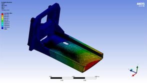
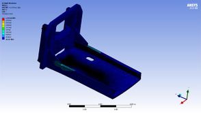
| − | + | From the prediction of the optimized results, the errors of the pallet rack shape variations of the E-AHF and KRG models are 0.5% and 0.5%, respectively. The errors of the stresses of the E-AHF and KRG models are 3.3% and 3.0%, respectively. The errors of the pallet rack masses of the E-AHF and KRG models are 1.2% and 1.2%, respectively. Taken together, from the analysis of the accuracy of model prediction, the KRG model undoubtedly has better adaptability and stronger performance. From the comparison between before and after optimization, the reduction of pallet rack deformations by E-AHF and KRG models is 17.2% and 16.7%. The reduction of pallet rack stresses by E-AHF and KRG models is 37.1% and 31.6%, and the reduction of pallet rack mass by E-AHF and KRG models are 1.2% and 1.2%, respectively. Taken together, the optimization design based on the E-AHF model is more excellent and adaptable to engineering examples. Therefore, the optimal solution obtained from the E-AHF model is brought into the simulation model to obtain the optimized results, as shown in [[#img-9|Figure 9]] . | |
| − | {| style=" | + | <div id='img-9'></div> |
| + | {| class="wikitable" style="margin: 0em auto 0.1em auto;border-collapse: collapse;width:auto;" | ||
| + | |-style="background:white;" | ||
| + | |align="center" | | ||
| + | {|style="margin: 0em auto 0.1em auto;width:auto;" | ||
| + | |+ | ||
|- | |- | ||
| − | | | + | |style="text-align: center;padding:10px;"| [[Image:Review_120867196377-image14.jpeg|294px]] |
| − | | | + | |style="text-align: center;padding:10px;"| [[Image:Review_120867196377-image15.jpeg|294px]] |
|- | |- | ||
| − | | | + | |style="text-align: center;font-size: 75%;padding-bottom:10px;"|(a) Deformation after optimization |
| − | | | + | |style="text-align: center;font-size: 75%;padding-bottom:10px;"|(b) Stress after optimization |
| + | |} | ||
|- | |- | ||
| − | | | + | | style="background:#efefef;text-align:left;padding:10px;font-size: 85%;"| '''Figure 9'''. Optimized cloud maps |
|} | |} | ||
| − | |||
===5.2 Global sensitivity analysis=== | ===5.2 Global sensitivity analysis=== | ||
| Line 625: | Line 626: | ||
| <math>f(x)={f}_{0}+\sum _{i}^{}{f}_{i}({x}_{i})+\sum _{i<j}^{}{f}_{ij}({x}_{i},{x}_{j})+</math><math>{f}_{1,2,\ldots ,n}({x}_{1},{x}_{2},\ldots ,{x}_{n})</math> | | <math>f(x)={f}_{0}+\sum _{i}^{}{f}_{i}({x}_{i})+\sum _{i<j}^{}{f}_{ij}({x}_{i},{x}_{j})+</math><math>{f}_{1,2,\ldots ,n}({x}_{1},{x}_{2},\ldots ,{x}_{n})</math> | ||
|} | |} | ||
| − | | style="text-align: center;width: 5px;text-align: right;white-space: nowrap;"| | + | | style="text-align: center;width: 5px;text-align: right;white-space: nowrap;"|(12) |
|} | |} | ||
| + | where <math display="inline">{x}_{i}</math> denotes the <math display="inline">i</math>-th variable and <math display="inline">{x}_{j}</math> denotes the <math display="inline">j</math>-th variable. | ||
| − | + | The total standard deviation and partial standard deviation of <math display="inline">f(x)</math> are, respectively: | |
| − | + | ||
| − | + | ||
{| class="formulaSCP" style="width: 100%;border-collapse: collapse;width: 100%;text-align: center;" | {| class="formulaSCP" style="width: 100%;border-collapse: collapse;width: 100%;text-align: center;" | ||
| Line 640: | Line 640: | ||
| <math>D=\int_{}^{}{f}^{2}(x)dx-{f}_{0}^{2}</math> | | <math>D=\int_{}^{}{f}^{2}(x)dx-{f}_{0}^{2}</math> | ||
|} | |} | ||
| − | | style="text-align: center;width: 5px;text-align: right;white-space: nowrap;"| | + | | style="text-align: center;width: 5px;text-align: right;white-space: nowrap;"|(13) |
| + | |- | ||
| + | |} | ||
| + | |||
| + | {| class="formulaSCP" style="width: 100%;border-collapse: collapse;width: 100%;text-align: center;" | ||
|- | |- | ||
| | | | ||
| Line 647: | Line 651: | ||
| <math>{D}_{{i}_{1}\ldots {i}_{s}}=\int_{}^{}{f}_{{i}_{1}\ldots {i}_{s}}^{2}(x)d{x}_{{i}_{1}}\ldots d{x}_{{i}_{s}}</math> | | <math>{D}_{{i}_{1}\ldots {i}_{s}}=\int_{}^{}{f}_{{i}_{1}\ldots {i}_{s}}^{2}(x)d{x}_{{i}_{1}}\ldots d{x}_{{i}_{s}}</math> | ||
|} | |} | ||
| − | | style="text-align: center;width: 5px;text-align: right;white-space: nowrap;"| | + | | style="text-align: center;width: 5px;text-align: right;white-space: nowrap;"|(14) |
|} | |} | ||
| − | + | The first-order sensitivity indices for each variable are: | |
{| class="formulaSCP" style="width: 100%;border-collapse: collapse;width: 100%;text-align: center;" | {| class="formulaSCP" style="width: 100%;border-collapse: collapse;width: 100%;text-align: center;" | ||
| Line 660: | Line 664: | ||
| <math>{S}_{i}=\frac{{D}_{{i}_{1}\ldots {i}_{s}}}{D}</math> | | <math>{S}_{i}=\frac{{D}_{{i}_{1}\ldots {i}_{s}}}{D}</math> | ||
|} | |} | ||
| − | | style="text-align: center;width: 5px;text-align: right;white-space: nowrap;"| | + | | style="text-align: center;width: 5px;text-align: right;white-space: nowrap;"|(15) |
|} | |} | ||
| + | where <math display="inline">{S}_{i}</math> denotes the first-order sensitivity index of the <math display="inline">i</math>-th variable. The global sensitivity index <math display="inline">{S}_{ti}</math> of the <math display="inline">i</math>-th variable is then the sum of the sensitivity indices of each order of the <math display="inline">i</math>-th variable. | ||
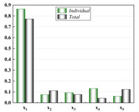
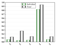
| − | + | Based on the E-AHF model, the GSA analysis of the pallet rack is carried out, and the results are shown in [[#img-10|Figure 10]]. It can be clearly seen that the channel height <math display="inline">{x}_{1}</math> has the greatest influence on the shape variables of the pallet rack, and both the first-order sensitivity index and the global sensitivity index are much higher than the remaining four design variables; whereas, the one that has a greater influence on the stress of the pallet rack is the channel flange thickness <math display="inline">{x}_{4}</math>, and its sensitivity index is also much higher than that of the other four variables; whereas, for the pallet rack mass, it can be seen that, except for the web thickness <math display="inline">{x}_{3}</math>, the rest of the design variables all have a greater influence. In summary, in the design of a pallet rack, the highest priority should be given to the height of channel steel <math display="inline">{x}_{1}</math> which has the greatest influence on its shape variables, to ensure the overall safety and pressure resistance of the lifting platform. | |
| − | < | + | <div id='img-10'></div> |
| − | + | {| class="wikitable" style="margin: 0em auto 0.1em auto;border-collapse: collapse;width:auto;" | |
| − | {| style=" | + | |-style="background:white;" |
| + | |align="center" | | ||
| + | {|style="margin: 0em auto 0.1em auto;width:auto;" | ||
| + | |+ | ||
|- | |- | ||
| − | | | + | |style="text-align: center;padding:10px;"| [[Image:Review_120867196377-image16-c.png|200px]] |
| − | | | + | |style="text-align: center;padding:10px;"| [[Image:Review_120867196377-image17-c.png|200px]] |
| − | | | + | |style="text-align: center;padding:10px;"| [[Image:Review_120867196377-image18-c.png|200px]] |
|- | |- | ||
| − | | | + | |style="text-align: center;font-size: 75%;padding-bottom:10px;"|(a) GSA for deformation |
| − | | | + | |style="text-align: center;font-size: 75%;padding-bottom:10px;"|(b) GSA for stress |
| − | | | + | |style="text-align: center;font-size: 75%;padding-bottom:10px;"|(c) GSA for quality |
| + | |} | ||
|- | |- | ||
| − | | | + | | style="background:#efefef;text-align:left;padding:10px;font-size: 85%;"| '''Figure 10'''. GSA based on E-AHF model |
|} | |} | ||
| Line 687: | Line 696: | ||
==Acknowledgment== | ==Acknowledgment== | ||
| − | The research was supported by the Longgang Institute of Zhejiang Sci-Tech University(LGYJY2021004). | + | The research was supported by Zhejiang University of Technology Project(11132932612108), the Longgang Institute of Zhejiang Sci-Tech University(LGYJY2021004), and Zhejiang Province Science and Technology Plan Project (2023C01174). |
==References== | ==References== | ||
| − | [1] Chen | + | <div class="auto" style="text-align: left;width: auto; margin-left: auto; margin-right: auto;font-size: 85%;"> |
| + | |||
| + | [1] Chen G.D. Multi-objective optimization method based on metamodel and its applications in vehicle body design. Ph.D. Thesis, Hunan University, Changsha, 2012. | ||
| − | [2] Queipo | + | [2] Queipo N.V., Haftka R.T., Shyy W., Goel T., Vaidyanathan R., Tucker P.K. Surrogate-based analysis and optimization. Progress in Aerospace Sciences, 41(1):1-28, 2005. |
| − | [3] Song | + | [3] Song X., Sun G., Li G., Gao W., and Li Q. Crashworthiness optimization of foam-filled tapered thin-walled structure using multiple surrogate models. Structural and Multidisciplinary Optimization, 47(2):221-231, 2013. |
| − | [4] Chen | + | [4] Chen W., Zhou X., Wang H., Wang W. Multi-objective optimal approach for injection molding based on surrogate model and particle swarm optimization algorithm. Journal of Shanghai Jiaotong University, 15(1):88-93, 2010. |
| − | [5] Jiang | + | [5] Jiang P., Zhou Q., Shao, X. Surrogate model-based engineering design and optimization. Series on Springer Tracts in Mechanical Engineering, Springer Singapore, pp. 240, 2020. |
| − | [6] Ruan | + | [6] Ruan X., Jiang P., Zhou Q. et al. Variable-fidelity probability of improvement method for efficient global optimization of expensive black-box problems. Structural and Multidisciplinary Optimization, 62(6):3021-3052, 2020. |
| − | [7] Meng | + | [7] Meng Z., Zhang Z., Zhou H., Chen H., Yu B. Robust design optimization of imperfect stiffened shells using an active learning method and a hybrid surrogate model. Engineering Optimization, 52(12):2044-2061, 2020. |
| − | [8] Yondo | + | [8] Yondo R., Andres E., Valero E. A review on design of experiments and surrogate models in aircraft real-time and many-query aerodynamic analyses. Progress in Aerospace Sciences, 96:23-61, 2018. |
| − | [9] Zhang | + | [9] Zhang X., Xie F., Ji T., Zhu Z., Zheng Y. Multi-fidelity deep neural network surrogate model for aerodynamic shape optimization. Computer Methods in Applied Mechanics and Engineering, 373, 113485, 2021. |
| − | [10] Kushner | + | [10] Kushner H.J. A new method of locating the maximum point of an arbitrary multipeak curve in the presence of noise. Journal of Basic Engineering, 86(1):97-106, 1964. |
| − | [11]Jones | + | [11]Jones D.R., Schonlau M., Welch W.J. Efficient global optimization of expensive black-box functions. Journal of Global Optimization, 13:455-492, 1998. |
| − | [12] Zeng | + | [12] Zeng F., Zhou J. Optimization strategy for dynamic metamodel integrating minimize lower confidence bound and trust region. Journal of Mechanical Engineering, 53(13):170-178, 2017. |
| − | [13] Kleijnen | + | [13] Kleijnen J.P.C. Expected improvement in efficient global optimization through bootstrapped kriging. Journal of Global Optimization, 54(1):59-73, 2012. |
| − | [14] Chaudhuria | + | [14] Chaudhuria A., Haftka R.T., Ifju P., Chang K., Tyler C., Schmitz T. Experimental flapping wing optimization and uncertainty quantification using limited samples. Structural & Multidisciplinary Optimization, 51(4):957–970, 2015. |
| − | [15] Song | + | [15] Song X., Lv L., LI J., Sun W., Zhang J. An advanced and robust ensemble surrogate model: Extended adaptive hybrid functions. Journal of Mechanical Design, 140(4):041402, 2018. |
| − | [16] Mckay | + | [16] Mckay M.D., Beckman R.J., Conover W.J. A comparison of three methods for selecting values of input variables in the analysis of output from a computer code. Technometrics, 21(2):239-245, 1979. |
| − | [17] | + | [17] Gunst R.F., Mason R.L. Fractional factorial design. Wiley Interdiscipl. Rev. Comput. Stat., 1(2):234–244, 2009. |
| − | [18] Boddy | + | [18] Boddy R., Smith G. Effective experimentation: For scientists and technologists. John Wiley & Sons, New York, pp. 270, 2010. |
| − | [19] Turner | + | [19] Turner C.J., Crawford R.H., Campbell M.I. Multidimensional sequential sampling for NURBs-based metamodel development. Engineering with Computers, 23:155-174, 2007. |
| − | [20] Cox | + | [20] Cox D.D., John S. SDO: A statistical method for global optimization. IEEE International Conference on Systems, Man and Cybernetics, Chicago, IL, Vol. 2, pp. 1241–1246, 1992. |
| − | [21] Sobol′ | + | [21] Sobol′ I.M. Global sensitivity indices for nonlinear mathematical models and their Monte Carlo estimates. Mathematics and Computers in Simulation, 55:271-280, 2001. |
Latest revision as of 01:01, 6 December 2023
Abstract
As an important part of the lifting platform of pallet forklift trucks, how to reduce the deformation of the pallet rack under working conditions while reducing the mass to ensure the safety performance of forklift trucks is the most concerning issue in the design of forklift truck structure. The pallet rack structure is complex, and optimizing simulation using traditional high-precision simulation models takes much time and effort. Therefore, this paper takes the lifting platform of an unmanned AVG forklift truck as the research object and establishes a parametric model of the pallet rack using the 3D modelling software SolidWorks and the finite element analysis software ANSYS to carry out static analysis of it. Optimization design variables are selected, a single surrogate model and ensemble surrogate model are chosen for various surrogate model techniques, a small number of sample points are used to construct a low-precision model, and adaptive infilling technology is used to improve the model accuracy, and the structure is optimized, and the results show that, while the pallet rack structure meets the requirements of light weight and strength, the mass is reduced by 1.2%, and the morphology is reduced by 17.2%. Moreover, a global sensitivity analysis of each design parameter was carried out under the guidance of the surrogate model, highlighting the most influential design variable as the height of the channel steel and establishing the design variables that should be taken into account in the structural design. This paper compares the performance of the mainstream single-surrogate model and ensemble-surrogate model as well as the adaptive infilling strategy in engineering design and proves that the surrogate model optimization method has a certain guiding significance for the structural optimization design of pallet racking.
Keywords: Optimization design, surrogate models, pallet racks, DoEs, infilling
1. Introduction
AGV forklift is an important unmanned material handling robot under the trend of intelligent industry, and its mature technology makes it widely used in stations, ports, airports, factories and warehouses, AGV forklifts are highly efficient equipment for mechanised loading and unloading, stacking and short-distance transport. Among them, a pallet forklift can ensure the stability of the material itself in the case of uneven road surfaces and heavy loads of forklifts, which is an important part of the forklift branch. Therefore, AGV pallet forklift is the current research focus of unmanned material handling robots.As an important component of the pallet forklift working device, the pallet rack is the executor of the forklift to realize the handling function and the focus point of value embodiment. Its performance directly affects the efficiency of the forklift. Traditionally, the optimal design of pallet rack is mainly done through computer-aided design, and good results are obtained by simulation optimization, but there are many disadvantages in the simulation itself: the simulation process is time-consuming, and there is a lack of optimization algorithms for the time-consuming simulation, which results in the whole simulation process needing a lot of time and computational costs. The structural design of pallet racks involves multiple variables and highly nonlinear relationships, in this context, the surrogate modelling technique, which has a small amount of computation and is based on a small amount of sample data, is an excellent choice [1], and optimization based on the surrogate model technique can reduce the computation time and improve the optimization efficiency.
In recent years, the field of surrogate modelling has continued to develop, giving rise to numerous new methods and varieties, which have achieved excellent results in the fields of mechanical, materials, fluid and other engineering fields. Queipo et al. [2] provide a comprehensive discussion of the fundamental issues that arise from surrogate model-based analysis and optimization. In 2012, Song et al. [3] used multiple surrogate models to perform collisional foam-filled conical thin-walled structure optimization, and the results show that different surrogate model approaches produce different results for the final collision optimization design. Chen et al. [4] performed a multi-objective optimization design of an injection model based on the KRG model and the particle swarm optimization algorithm. In 2020, Jiang et al. [5,6] systematically elaborated on the application of surrogate models in the field of engineering and used a variable fidelity surrogate model to design the micro air vehicle fuselage as well as reinforced cylindrical shells. In 2020, Meng et al. [7] optimized the robust design of incomplete reinforcing bars based on an ensemble surrogate model. Yondo et al. [8] compared the surrogate model approach and the experimental design approach in the aerodynamic analysis of a flight vehicle try and introduced the optimization method based on the surrogate model. In 2021, Zhang et al. [9] proposed an optimization framework based on a multi-fidelity surrogate model by correlating the configuration parameters of an aircraft with its start-up performance.
Prediction is one of the most important functions of the surrogate model, and one of the important methods to improve the prediction accuracy of the surrogate model is to update the surrogate model by infilling the criterion. The more commonly used mainstream infilling criteria are the maximizing the probability of improvement (PoI) [10] criterion and maximizing expectation improvement (EI) [11] criterion, of which the EI method has better global search performance and a wide range of application scenarios and has become one of the most mainstream infilling criteria, which also has a lot of applications in engineering design. Zeng and Zhou [12] proposed a KRG model optimization method integrating LCB and trust domain and successfully applied it to the design optimization of I-beam. Kleijnen [13] proposed a bootstrap EI method, which can realize the multi-point infilling process based on EI and improve the modelling efficiency. Chaudhuri et al. [14] ensemble EI and PoI criteria to update the surrogate model every time by obtaining multiple sample points obtain multiple sample points to update the surrogate model and apply the method to the optimized design of vibrating wings. Liu et al. [16] converted the classical four criteria EI, PI, LCB, and MP into an infilling criterion with constraints and applied it to the wing and aerodynamic inverse design problems, and obtained better results.
In this paper, an unmanned AGV forklift truck is selected as the research object, focusing on the analysis and improvement of the pallet rack part of the forklift truck, to achieve lightweight under the premise of ensuring the structural strength and the optimization makes the forklift truck have a higher structural strength, a better loading capacity, and a lighter mass. At the same time, to compare the difference between the ensemble surrogate model and the single surrogate model in engineering applications, this paper chooses the single surrogate model represented by the Kriging(KRG) [10] model and the ensemble surrogate model represented by the extended adaptive hybrid functions(E-AHF) [15] to optimize the design and analysis of the forklift truck pallet racks, respectively. Among them, the KRG model, as one of the typical single-surrogate models, is essentially a linearly weighted combination of information about known points in order to predict the position information within a certain range. Unlike the rest of the single surrogate models, the KRG model has a better local prediction ability due to the correlation function, good continuity and derivability, and good approximation for nonlinear complex problems. The E-AHF ensemble surrogate model, one of the newly proposed ensemble surrogate models in recent years, has excellent predictive ability due to its extensive model library and the excellent weighting method used. It has better global performance for highly nonlinear problems. Therefore, the above two surrogate models are chosen to represent their respective fields. In order to further reduce the cost of the simulation model, this paper chooses to construct the low-precision surrogate model with less sample points. To further reduce the cost of the simulation model, this paper chooses to construct a low-precision surrogate model with fewer sample points and to improve the model accuracy by using the adaptive infilling criterion to reduce the number of times the simulation software is used. Finally, the most suitable model is selected from multiple error criteria.
The rest of the paper is arranged as follows: Section 2 briefly introduces the mathematical principles and related formulas involved in this paper, which are mainly related to the calculation of the surrogate model; Section 3 introduces the research object of this paper, the unmanned AGV stacker truck, and constructs the related finite element model; Section 4 constructs the relevant surrogates for the pallet rack with a single model and an ensemble model respectively; Section 5 compares the performance of the two surrogate models in this optimal design, selects the most suitable model, and based on which the design and optimization of the pallet rack are implemented; and the conclusions of this study are discussed in Section 6.
2. Mathematical theories
2.1 KRG model
The KRG model [10], originally proposed by the South African geologist Danie Krige in 1951 for the exploration of mineral reserves, is an uncertainty-free interpolation model for estimating standard deviation minimization, which uses a covariance-controlled Gaussian process to generate continuous functions.
A generic KRG model can be expressed as follows:
|
|
(1) |
where is the response function for the region of interest, is a polynomial function used as an approximation to the underlying functional model, and denotes a stochastic process with uncertainty in the mean of . The KRG model is an interpolation method through each sample point.
In this paper, we use the Gaussian correlation function:
|
|
(2) |
where is the number of design variables, and are parameters that vary flexibly with the variables, and is the distance between and concerning the -th variable.
The predicted value of at test point is formulated as follows:
|
|
(3) |
where is a column vector of sample response values, and when is a constant vector, is a column vector of length with all elements of 1. is the correlation vector between the test point and the sample points.
2.2 Ensemble surrogate models
Ensemble surrogate models are obtained by superimposing the weights of several individual surrogate models, and the key lies in solving for the appropriate weight coefficients. The current ensemble surrogate models can be divided into two types, namely, average weights and adaptive weights, according to the different forms of weight coefficients. This paper focuses on the adaptive weighted ensemble surrogate model used.
In 2018, Song et al. [15] proposed an ensemble surrogate model: Extended Adaptive Hybrid Functions (E-AHF). Three steps are proposed for model screening and adaptive weight calculation.
Step 1. Local measure estimation
|
|
(4) |
where denotes the constant process variance of a Gaussian field, and is the correlation matrix with the elements.
Step 2. Probability estimation
The baseline model can represent the global trend of the hybrid surrogate model, due to its high accuracy across the entire design space. Therefore, this prediction by the baseline model can be deemed as an expected value of the hybrid model. With the local prediction estimation obtained from the previous local measure estimation, the probability coefficient of each individual surrogate model can be calculated by
|
|
(5) |
where is the prediction value of the baseline model at the -th sample point, is the probability coefficient associated with the -th individual surrogate model, and is the local prediction estimation at the -th sample point.
Step 3. Local weight determination
With the probability coefficient assigned to each surrogate model, the weight factors can be computed by
|
|
(6) |
As is a function of the input vector , the weight factors obtained for each individual surrogate model is adaptive to the input vector as well.
2.3 Maximizing EI
Unlike the PoI strategy, which focuses on the probability of improvement, the EI strategy is related to the amount of improvement expected to be obtained when adding a filling point and given a filling point, the EI is expressed in terms of a Gaussian error function as follows:
|
|
(7) |
It is observed from equations and that the expressions for both PoI and EI strategies contain global terms () and local terms (), indicating that both approaches can balance global exploration and local exploitation to some extent.
2.4 Performance criterion
In this paper, we use two criteria to evaluate the accuracy of the model. That is, the coefficient of determination is used as a global evaluation metric; the normalized max absolute error (NMAE) is used as a local evaluation metric to evaluate the global and local performance of different infilling strategies, respectively
|
|
(8) |
|
|
(9) |
where denotes the true response at the -th test point, and the predicted value of the model built by the surrogate model approach at the -th test point is , and is the mean value of the true response at all test points, ntest denotes the number of test points.
Usually, ranges from 0 to 1, and a larger d or a smaller NMAE means more accurate surrogates. When is negative, it represents that the constructed surrogate model is trending opposite to the true model.
3. Establishment of finite element model of pallet rack
3.1 Structure of pallet racks
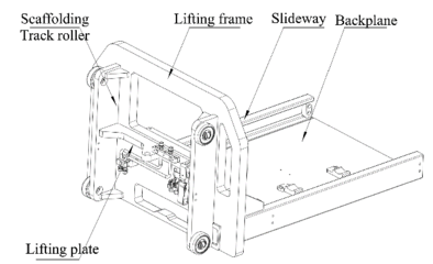
The AGV forklift involved in this paper is a battery-powered, unmanned material handling vehicle with automatic guidance, and its lifting platform consists of a pallet rack, two-wheel frame plates, a lifting plate, a guide rail, and a base plate, as shown in Figure 1. Among them, the pallet rack, as the structural main body of the lifting platform, is used to bear all the weight of the pallet containing materials and the loaded materials and is all the force components of the lifting platform, as well as the key structure of the lifting platform. As an important part of the AGV forklift, the reasonable design of the lifting platform directly determines the working ability of the forklift. In daily operation, the pallet rack will be subjected to more complicated forces in repeated lifting operations. Therefore, the structural design and optimization of the pallet rack will directly lead to the degree of deformation and reliability of each component of the AGV forklift in the course of operation, affecting the safety performance and working efficiency of the lifting platform, which in turn seriously affects the overall working life of the forklift.
|
| Figure 1. Structure of lifting platform |
3.2 Simulation analysis of pallet racks
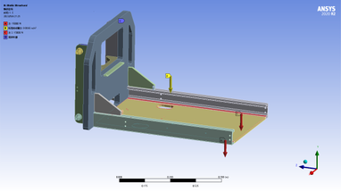
A 3-D model of the pallet rack was built using SolidWorks and imported into ANSYS for static analysis. The material used for the pallet rack is 25MnV alloy steel, Set the material properties in Workbench: density 7850 , modulus of elasticity Mpa, Poisson's ratio of 0.3. The free mesh division of the pallet rack is carried out, with a grid cell size of 10mm, and local encryption is carried out on the parts that are prone to stress concentration, and a total of 191599 mesh cells are generated with 424581 nodes. The main loads and constraints on the pallet rack include: fixed constraints on the lifting plate of the fixed pallet rack, which is used to limit the vertical displacement of the pallet rack; the downward pressure acting on the side plates of the channel steel , and the gravity of the pallet rack itself . The overall load diagram of the pallet rack is shown in Figure 2.
|
| Figure 2. Overall load diagram of pallet racks |
4. Constructing surrogate model for pallet racking
Surrogate model method is a mathematical analysis model method, which belongs to a branch of supervised machine learning, and has gained wide attention and research in many fields such as mechanical simulation, ecological modelling, geological statistics, artificial intelligence, etc., due to its ability to quickly and effectively achieve the approximate fitting of multidimensional variable complex systems based on limited data information. Surrogate modeling technology does not need to understand the physical meaning between input variables and output responses, and can only use the data itself to obtain an approximate mathematical model, so it can be applied to the optimization design and analysis where the physical meaning between the inputs and outputs is not clear, and the computational cost is high, and it has the advantages of good fitting accuracy, low cost, high efficiency, and so on. The application process of the surrogate model in engineering in general is shown in Figure 3, which mainly includes three modules: problem analysis, modelling analysis and result analysis.

|
| Figure 3. Flow of application of surrogate model in engineering |
4.1 Identification of design variables
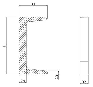
As the main stress structure of the pallet rack, the channel steel and diagonal reinforcement is an important structure to support the pallet rack frame and transfer its stress, and its strength also determines whether the forklift truck can complete the engineering transport work more efficiently and safely. Therefore, the structural optimization of channel steel as well as diagonal tie bars can further reduce the stress and deformation while ensuring the strength, reduce the mass, and improve the economy and overall stability. After clarifying the overall structural weaknesses, this paper selects four design variables for the channel section and five design variables for the thickness of the diagonal bar as the optimization parameters, as shown in Figure 4, which are the height , width , web thickness and flange thickness of the channel and the thickness of the diagonal bar , respectively. The range and initial values of the corresponding design variables are shown in Table 1.
|
| Figure 4. Schematic diagram of the design variables of the pallet racks |
| Design variables | Range of values (mm) | Initial value (mm) |
|---|---|---|
| Height of channel | 90~120 | 105 |
| Width of channel | 37~53 | 45 |
| Thickness of web | 6.5~8.5 | 7.5 |
| Flange thickness | 7.5~9 | 8.25 |
| Thickness of diagonal reinforcement | 12~20 | 16 |
4.2 Design of experiment
In the application of the surrogate model in engineering shown in Figure 4, the design of experiments (DoE) is the first step in constructing the surrogate model, and it is also the key step in constructing the surrogate model, the essence of which is to generate the sample points in the region of interest, and a good DoE method is able to extract more compliant sample points and to construct a more accurate model with a smaller amount of data. The DoE methods can be divided into static sampling and adaptive sampling. Static sampling, means that the training points needed to construct the surrogate model are extracted at one time. Currently, widely used static sampling methods include Latin hypercube sampling (LHS) [16], Fractional factorial design (FFD) [17] and central composite design (CCD) [18]. In static sampling, the training points are independent of the constructed surrogate model, i.e., static sampling cannot learn from known samples.
The adaptive infilling strategy is designed to overcome the limitations of static sampling independent models, using the results of the currently constructed surrogate model, and selecting new sample points that are more conducive to the construction of an accurate model through the "infilling strategy" to improve the accuracy of the surrogate model iteratively [19]. Typical infilling strategies include Statistical lower bound (SLB) [20] strategy, maximizing probability of improvement (PoI) strategy, maximizing expected improvement (EI) strategy, etc. The EI strategy has been used by most researchers, and the EI strategy has been used by most researchers. etc. Among them, the EI strategy has been confirmed by most studies to have better performance in local exploitation and global exploration, and it is one of the most widely used infilling strategies nowadays. In this paper, the EI strategy ischosen as the infilling strategy.
According to the process of constructing the surrogate model, after determining the range of design variables, LHS is used to select points for the experimental design, 60 points are selected, and the corresponding maximum stress and maximum deformations under the relevant loads are calculated using simulation, of which 10 groups of data are used to construct the low-precision surrogate model, and the remaining 50 groups of data are used as a database, which is used to provide response values for the new samples added at each iteration using the EI adaptive infilling strategy. The remaining 50 data sets are used as a database to provide response values for new sample points added at each iteration when using the EI adaptive infilling strategy, and the 50 data sets can also be used as a test set to examine the global and local accuracy ( and NMAE) of the constructed surrogate models. Figure 5 shows the distribution of the 60 groups of design variables in the design space, and it can be clearly seen that the training and test points are distributed in almost the whole design space with good space filling and projection, and the test and training points are interspersed with each other, which indicates that the sampling point analysis meets the requirements.
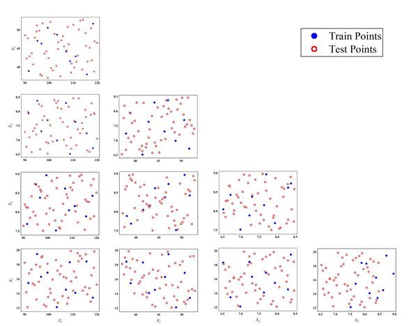
|
| Figure 5. Distribution of training and test points |
4.3 Constructing surrogate model for pallet racking
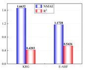
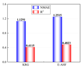
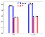
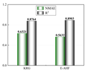
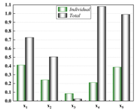
In order to better reduce the cost brought by simulation experiments, this paper uses the EI infilling method to gradually guide the updating of the model and improve the accuracy of the surrogate model, therefore, when constructing the surrogate model, 10 sets of data will be used to construct the low-precision single surrogate model KRG and the low-precision ensemble surrogate model E-AHF, respectively, and according to the flow of the modelling in Figure 3, the model will be judged based on the accuracy judging criterion ( and NMAE) for the accuracy, and use the EI strategy to iteratively improve the accuracy until the surrogate model reaches a usable accuracy (usually ), and in order to compare the performance of the single surrogate model and the ensemble surrogate model in this optimization, the construction of the surrogate model will be guided by the KRG model and the E-AHF model to construct the models of the design variables with respect to the deformation, mass, and stresses, respectively. The bar charts in Figure 6 show the performance of the two different models with 10 sample points with global metrics () and local metrics (NMAE) as references.
| ||||||
| Figure 6. Comparison of low precision surrogate models |
It is obvious through Figure 6 that 10 sample points are not capable of constructing a high-precision model, but in the case of limited data, the ensemble surrogate model E-AHF still exhibits higher accuracy, and the KRG model is superior in terms of scope of applicability and degree of accuracy in the single surrogate model, but the comprehensive comparison of the three response objectives of pallet racking's deformation, stress, and mass is not as good as the E-AHF model, whether it is in terms of global accuracy or local accuracy.
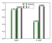
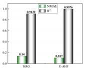
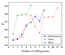
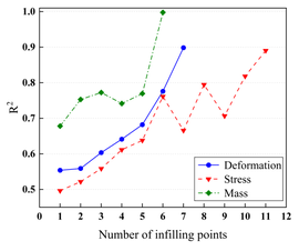
After the low-precision model is constructed, the EI strategy is used to guide the selection of new sample points based on the initial model, and one new sample point is selected to be added to the training set at each iteration until the model stops iterating when it reaches a usable accuracy. Figure 7 demonstrates a comparison of the accuracy of the KRG model and the E-AHF model after the convergence of the iterations. Figure 8 compares the number of sample points used to construct the model after reaching the usable accuracy for both models. It can be seen that the models constructed by both KRG and E-AHF reach high accuracy after the EI infilling strategy, but comparing the data in Figure 7, the E-AHF model still has an advantage in terms of global accuracy and local accuracy in deformation, stress and mass. Comparing the line graph in Figure 8, it can be seen that the same model that achieves , the E-AHF model can achieve the corresponding accuracy with fewer training points, which means that fewer times of the EI infilling strategy is used, and when put in the simulation experiments, it means that fewer times of the simulation are carried out, which saves the cost and time, and objectively proves the superiority of the ensemble surrogate model, which is represented by the E-AHF, compared with the single surrogate model. The exact number of additional sample points is shown in Table 2.
| ||||||
| Figure 7. Comparison of high-precision surrogate models |
| ||||
| Figure 8. Comparison of the number of infilling points for the two surrogate models |
| Response | KRG | E-AHF | ||
|---|---|---|---|---|
| Initial points | Additional points | Initial points | Additional points | |
| Deformation | 10 | 8 | 10 | 7 |
| Stress | 10 | 11 | 10 | 11 |
| Mass | 10 | 5 | 10 | 6 |
5. Optimization results and analysis
5.1 Definition of problem
The KRG model and the E-AHF model presented above were used instead of the simulation model for optimization and design. In the optimization of the entire pallet rack, deformation and mass are the two objectives that need to be paid attention to during the optimization process, but in fact, these two optimization objectives are contradictory to each other, as a less deformed structure is more rigid and corresponds to a higher mass, so it is difficult to balance the two ends of the spectrum during the design process. Reviewing the specific situation in engineering applications, it is not difficult to find that compared with lightweight, higher structural strength is the focus of design considerations, higher strength to ensure the safety factor of machinery in the project, as well as a longer working life, placed in this optimization design process, smaller deformation is the priority of the experimental findings of the conflict between the object.
Therefore, in this paper, we will calculate the optimal solution of the two constraint problems for the optimization objective and compare the experimental results to conclude with the same number of total constraints, which are stress constraints, deformation constraints, and mass constraints, respectively. Where [T] and [M] are the permitted values of deformation and mass respectively. Considering the specific application and working conditions, the geometries of non-standard channels and diagonal ties are constrained. For the optimization problem described below, this paper uses a single-objective Genetic algorithm (GA), and the optimization problem for the whole pallet rack is described as:
Question 1: Deformation constraints, stress constraints and dimensional constraints
|
(10) |
Question 2: Mass constraints, stress constraints and dimensional constraints
|
(11) |
where is the optimization objective, is the total deformation and is the total weight of the pallet rack structure.
The specific results of the two optimization problems are shown in Tables 3 and 4, respectively, and compare the predicted and true responses of the objective function and constraints. From the information in the table, it can be seen that the structural value derived from minimizing mass as the optimization objective with deformation and stress as constraints. Although the mass reduction is larger, the optimized resultant deformation and stress reduction is small, and this degree of lightweight has limited cost reduction in practical engineering applications, so the results of the optimization problem are not considered. On the other hand, the structural values derived by using mass and stress as constraints and minimizing deformation as the optimization objective not only better reduce the deformation of the pallet rack, but also significantly reduce the stress values, and even a small amount of reducing the mass of the pallet rack to meet the constraints is a better result. It is worth mentioning that in both optimization problems, the E-AHF model shows better performance in terms of all the indicators, and the constraint and objective functions written in its model give better guidance to the GA algorithm to get better results.
| Response | (mm) | (mm) | (mm) | (mm) | (mm) | Deformation (mm) | Stress (Mpa) | Quality (Kg) | |
|---|---|---|---|---|---|---|---|---|---|
| Before optimization | 105.0 | 45.0 | 7.5 | 8.25 | 16.0 | 2.39 | 648.1 | 252.7 | |
| After optimization | E-AHF | 107.6 | 41.9 | 6.5 | 8.0 | 12.3 | 2.19 | 446.0 | 246.3 |
| KRG | 105.8 | 44.3 | 6.9 | 8.1 | 12.2 | 2.25 | 428.2 | 246.9 | |
| Response | (mm) | (mm) | (mm) | (mm) | (mm) | Deformation (mm) | Stress (Mpa) | Quality (Kg) | |
|---|---|---|---|---|---|---|---|---|---|
| Before optimization | 105.0 | 45.0 | 7.5 | 8.25 | 16.0 | 2.39 | 648.1 | 252.7 | |
| After optimization | E-AHF | 109.8 | 42.7 | 6.9 | 8.7 | 13.2 | 1.98 | 407.7 | 249.7 |
| KRG | 110.6 | 41.8 | 6.7 | 8.6 | 13.9 | 1.99 | 443.6 | 249.7 | |
Based on the structural values derived from the optimization objective of minimizing deformation, in order to check the accuracy of the optimization results (incorporating stress, deformation and mass) predicted by the two surrogate models for the values calculated by the optimization algorithms, the optimization results were brought into the simulation model to obtain the real results and the errors were obtained by comparing them with the predicted values of the models, which are shown in Tables 5, 6 and 7, respectively.
| Optimal Model | After Optimization | Before Optimization | Decrease | ||
|---|---|---|---|---|---|
| Prediction | True | Error | |||
| E-AHF | 1.99 | 1.98 | 0.5% | 2.39 | 17.2% |
| KRG | 1.98 | 1.99 | 0.5% | 2.39 | 16.7% |
| Optimal Model | After Optimization | Before Optimization | Decrease | ||
|---|---|---|---|---|---|
| Prediction | True | Error | |||
| E-AHF | 394.3 | 407.7 | 3.3% | 648.1 | 37.1% |
| KRG | 430.5 | 443.6 | 3.0% | 648.1 | 31.6% |
| Optimal Model | After Optimization | Before Optimization | Decrease | ||
|---|---|---|---|---|---|
| Prediction | True | Error | |||
| E-AHF | 252.7 | 249.7 | 1.2% | 252.7 | 1.2% |
| KRG | 252.7 | 249.7 | 1.2% | 252.7 | 1.2% |
From the prediction of the optimized results, the errors of the pallet rack shape variations of the E-AHF and KRG models are 0.5% and 0.5%, respectively. The errors of the stresses of the E-AHF and KRG models are 3.3% and 3.0%, respectively. The errors of the pallet rack masses of the E-AHF and KRG models are 1.2% and 1.2%, respectively. Taken together, from the analysis of the accuracy of model prediction, the KRG model undoubtedly has better adaptability and stronger performance. From the comparison between before and after optimization, the reduction of pallet rack deformations by E-AHF and KRG models is 17.2% and 16.7%. The reduction of pallet rack stresses by E-AHF and KRG models is 37.1% and 31.6%, and the reduction of pallet rack mass by E-AHF and KRG models are 1.2% and 1.2%, respectively. Taken together, the optimization design based on the E-AHF model is more excellent and adaptable to engineering examples. Therefore, the optimal solution obtained from the E-AHF model is brought into the simulation model to obtain the optimized results, as shown in Figure 9 .
| ||||
| Figure 9. Optimized cloud maps |
5.2 Global sensitivity analysis
Global sensitivity analysis (GSA) is the study of the effects of simultaneous changes in different design variables throughout the design space on a system or model, with the aim of implementing dimensionality reduction and simplifying the model in high-dimensional cases. The most representative of GSA, Sobol global sensitivity analysis, which is a standard deviation-based sensitivity analysis method, is used in this study [21]. This method can simultaneously calculate the first-order sensitivity index and global sensitivity index of design variables, in which the first-order sensitivity index indicates the impact of individual design variables, while the global sensitivity index takes into account the interactions between individual variables. Its specific calculation method is as follows.
Given any product function in n-dimensional space, it can be expressed as:
|
|
(12) |
where denotes the -th variable and denotes the -th variable.
The total standard deviation and partial standard deviation of are, respectively:
|
|
(13) |
|
|
(14) |
The first-order sensitivity indices for each variable are:
|
|
(15) |
where denotes the first-order sensitivity index of the -th variable. The global sensitivity index of the -th variable is then the sum of the sensitivity indices of each order of the -th variable.
Based on the E-AHF model, the GSA analysis of the pallet rack is carried out, and the results are shown in Figure 10. It can be clearly seen that the channel height has the greatest influence on the shape variables of the pallet rack, and both the first-order sensitivity index and the global sensitivity index are much higher than the remaining four design variables; whereas, the one that has a greater influence on the stress of the pallet rack is the channel flange thickness , and its sensitivity index is also much higher than that of the other four variables; whereas, for the pallet rack mass, it can be seen that, except for the web thickness , the rest of the design variables all have a greater influence. In summary, in the design of a pallet rack, the highest priority should be given to the height of channel steel which has the greatest influence on its shape variables, to ensure the overall safety and pressure resistance of the lifting platform.
| ||||||
| Figure 10. GSA based on E-AHF model |
6. Conclusion
Taking the pallet rack of the lifting platform of the unmanned AGV stacker truck as the research object, the parametric design of the pallet rack is carried out by using SolidWorks and ANSYS, and then the design variables are selected, the design space is determined, and 60 sample points are selected by using the LHS method, of which 10 are used as a group for constructing an ensemble surrogate model represented by the E-AHF and a single surrogate model represented by KRG, the remaining 50 sample points are used as a group as a sample point library for the EI plus point strategy to improve the accuracy of the model by EI guidance, and the accuracy of two evaluation criteria can be tested. The remaining 50 sample points are used as the sample point bank for the EI infilling strategy, which is used to improve the accuracy of the model through the EI guidance, and at the same time, the accuracy of the constructed surrogate model can be examined by comparing the two evaluation criteria, which include the global and local indicators. Stress, mass and deformation are modelled using the two surrogate models, and two unused optimization problems with stress and deformation as constraints, and stress and mass as constraints are established, and Matlab Optimization Toolbox is used to optimize the models and compare the results of the two optimization problems, which show that the optimized mass has been reduced by 1.2%, and the deformation variable has been reduced by 17.2% compared with the initial deformation variable, which fully meets the objectives of the design, It fully meets the objectives of the optimized design. Finally, the E-AHF model is used as the basis for the global sensitivity analysis of the five design variables, and it is found that the most important shape variable is the length of the channel, which highlights the application of the surrogate model in the global sensitivity analysis, and at the same time provides a new research solution for the optimization of the forklift truck lifting platform.
Acknowledgment
The research was supported by Zhejiang University of Technology Project(11132932612108), the Longgang Institute of Zhejiang Sci-Tech University(LGYJY2021004), and Zhejiang Province Science and Technology Plan Project (2023C01174).
References
[1] Chen G.D. Multi-objective optimization method based on metamodel and its applications in vehicle body design. Ph.D. Thesis, Hunan University, Changsha, 2012.
[2] Queipo N.V., Haftka R.T., Shyy W., Goel T., Vaidyanathan R., Tucker P.K. Surrogate-based analysis and optimization. Progress in Aerospace Sciences, 41(1):1-28, 2005.
[3] Song X., Sun G., Li G., Gao W., and Li Q. Crashworthiness optimization of foam-filled tapered thin-walled structure using multiple surrogate models. Structural and Multidisciplinary Optimization, 47(2):221-231, 2013.
[4] Chen W., Zhou X., Wang H., Wang W. Multi-objective optimal approach for injection molding based on surrogate model and particle swarm optimization algorithm. Journal of Shanghai Jiaotong University, 15(1):88-93, 2010.
[5] Jiang P., Zhou Q., Shao, X. Surrogate model-based engineering design and optimization. Series on Springer Tracts in Mechanical Engineering, Springer Singapore, pp. 240, 2020.
[6] Ruan X., Jiang P., Zhou Q. et al. Variable-fidelity probability of improvement method for efficient global optimization of expensive black-box problems. Structural and Multidisciplinary Optimization, 62(6):3021-3052, 2020.
[7] Meng Z., Zhang Z., Zhou H., Chen H., Yu B. Robust design optimization of imperfect stiffened shells using an active learning method and a hybrid surrogate model. Engineering Optimization, 52(12):2044-2061, 2020.
[8] Yondo R., Andres E., Valero E. A review on design of experiments and surrogate models in aircraft real-time and many-query aerodynamic analyses. Progress in Aerospace Sciences, 96:23-61, 2018.
[9] Zhang X., Xie F., Ji T., Zhu Z., Zheng Y. Multi-fidelity deep neural network surrogate model for aerodynamic shape optimization. Computer Methods in Applied Mechanics and Engineering, 373, 113485, 2021.
[10] Kushner H.J. A new method of locating the maximum point of an arbitrary multipeak curve in the presence of noise. Journal of Basic Engineering, 86(1):97-106, 1964.
[11]Jones D.R., Schonlau M., Welch W.J. Efficient global optimization of expensive black-box functions. Journal of Global Optimization, 13:455-492, 1998.
[12] Zeng F., Zhou J. Optimization strategy for dynamic metamodel integrating minimize lower confidence bound and trust region. Journal of Mechanical Engineering, 53(13):170-178, 2017.
[13] Kleijnen J.P.C. Expected improvement in efficient global optimization through bootstrapped kriging. Journal of Global Optimization, 54(1):59-73, 2012.
[14] Chaudhuria A., Haftka R.T., Ifju P., Chang K., Tyler C., Schmitz T. Experimental flapping wing optimization and uncertainty quantification using limited samples. Structural & Multidisciplinary Optimization, 51(4):957–970, 2015.
[15] Song X., Lv L., LI J., Sun W., Zhang J. An advanced and robust ensemble surrogate model: Extended adaptive hybrid functions. Journal of Mechanical Design, 140(4):041402, 2018.
[16] Mckay M.D., Beckman R.J., Conover W.J. A comparison of three methods for selecting values of input variables in the analysis of output from a computer code. Technometrics, 21(2):239-245, 1979.
[17] Gunst R.F., Mason R.L. Fractional factorial design. Wiley Interdiscipl. Rev. Comput. Stat., 1(2):234–244, 2009.
[18] Boddy R., Smith G. Effective experimentation: For scientists and technologists. John Wiley & Sons, New York, pp. 270, 2010.
[19] Turner C.J., Crawford R.H., Campbell M.I. Multidimensional sequential sampling for NURBs-based metamodel development. Engineering with Computers, 23:155-174, 2007.
[20] Cox D.D., John S. SDO: A statistical method for global optimization. IEEE International Conference on Systems, Man and Cybernetics, Chicago, IL, Vol. 2, pp. 1241–1246, 1992.
[21] Sobol′ I.M. Global sensitivity indices for nonlinear mathematical models and their Monte Carlo estimates. Mathematics and Computers in Simulation, 55:271-280, 2001.Document information
Published on 27/10/23
Accepted on 17/10/23
Submitted on 14/09/23
Volume 39, Issue 4, 2023
DOI: 10.23967/j.rimni.2023.10.005
Licence: CC BY-NC-SA license
Share this document
Keywords
claim authorship
Are you one of the authors of this document?
