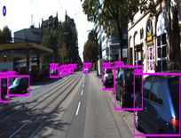
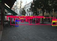
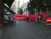
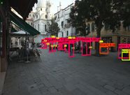
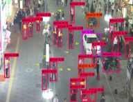
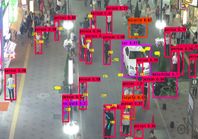
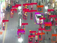
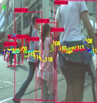
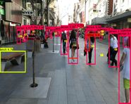
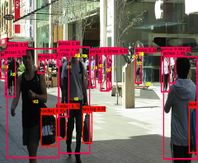
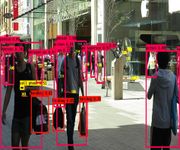
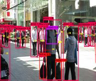
(Tag: Visual edit) |
|||
| (51 intermediate revisions by 3 users not shown) | |||
| Line 16: | Line 16: | ||
| − | <span style="text-align: center; font-size: 75%;">1, Guangdong Atv Academy For Performing Arts, Guangdong, China | + | <span style="text-align: center; font-size: 75%;"> |
| + | 1, Guangdong Atv Academy For Performing Arts, Guangdong, China | ||
2, Department of Computer Science, Baoji University of Arts and Sciences, Baoji, China | 2, Department of Computer Science, Baoji University of Arts and Sciences, Baoji, China | ||
| Line 26: | Line 27: | ||
'''*''' Correspondence: renchengjuan163[mailto:@163.com; @163.com;] | '''*''' Correspondence: renchengjuan163[mailto:@163.com; @163.com;] | ||
--> | --> | ||
| + | ==Abstract== | ||
| − | + | In multi-object tracking of Intelligent Transportation System, there are objects of different sizes in images or videos, especially pedestrian and traffic lights with low resolution . Meantime, objects are subject to occlusion and loss in object tracking. All of the above mentioned situations may lead to unsatisfactory multi-object tracking results. Attracted by the effect of deep convolution neural networks, the paper proposes a multi-object tracking network, CNN-based Multi-Object Tracking Networks with Position Correction and IMM (CNN_PC_IMM) to solve those problems. Our proposed method consists of object detection module and object tracking module. Compared to other networks, our proposed network has several main contributions that play an essential role in achieving state-of-the-art object tracking performance. In detection phase, feature fusion technique is used. We add a scale branch to the YOLOv3 network to increase the accuracy of small object prediction, and import a residual structure to enhance gradient propagation and avoid gradient disappearance or explosion for the whole network. In addition, we determine the size of the anchor box based on the size of the object in the dataset to better detection and tracking the objects. In tracking phase, IMM is used to calculate the motion state information of the object at a certain moment. Next, the optimization algorithm is proposed to fine-tune object position when the tracking object is occluded due to dense multi-object in traffic scenes or lost due to incomplete object information. Finally, experimental results and analysis are performed on MOT16 benchmark dataset with several popular tracking algorithms used to compare the performance with the proposed algorithm in the paper. It is demonstrated that the proposed algorithm has better performance on MOPA, MOTP, ML. | |
| − | '''Keywords | + | '''Keywords''': Intelligent transportation system, multi-object tracking, deep convolution neural networks, YOLOv3, IMM |
==1. Introduction== | ==1. Introduction== | ||
| Line 35: | Line 37: | ||
With the further improvement of people's material and cultural levels in modern society, vehicles have gradually developed into a consumer product needed by the public in daily life. However, along with the yearly increase the total number of vehicles come a series of serious traffic safety and traffic congestion problems in cities. For the prospective planning and development of each city, to reduce the occurrence of traffic accidents and traffic congestion, experts and scholars in industry and academia have invested a lot of human and material resources in the exploration of Intelligent Transportation Systems. | With the further improvement of people's material and cultural levels in modern society, vehicles have gradually developed into a consumer product needed by the public in daily life. However, along with the yearly increase the total number of vehicles come a series of serious traffic safety and traffic congestion problems in cities. For the prospective planning and development of each city, to reduce the occurrence of traffic accidents and traffic congestion, experts and scholars in industry and academia have invested a lot of human and material resources in the exploration of Intelligent Transportation Systems. | ||
| − | Multiple Object Tracking (MOT) also known as Multi-Object Tracking (MTT) is a computer vision task that seeks to optimize the analysis of video to identify and track objects belonging to more than one category [1, 2]. Multi-object tracking is an important part of the unmanned system perception algorithm. It not only provides data information of multiple spatio-temporal points and positions for multi-object motion objects, which gets the specific running state trajectory of each object. It also supplies highly informative data for object scene understanding. For example, the object motion contains information such as the acceleration and time of the motion of the corresponding object, the start-stop, and duration information of the acceleration in the trajectory which indicates when the object has entered and left the scene. The implicit information of the trajectory can also indirectly express the behavioral motility and behavioral psychological characteristics of each object, which can offer significant data for high-level computerized motion visual recognition such as behavioral feature analysis and behavioral feature prediction. In addition, rich message can be obtained by analyzing the motion state of each object, such as acquiring the number of objects that exist in a specific area over a while, the relationship between each object, etc. Therefore, multi-object tracking technology has important research and application value in Intelligent Transportation System. Traditional multi-object tracking involves three main elements, appearance model, motion model, and online update mechanism [3]. The implementation stage of traditional multi-object tracking includes constructing the initial appearance model, in which the initial area is obtained by object detection methods, etc.. And then, the corresponding features and the model are obtained by using the motion model to predict and analyze the area where the object is likely to appear. Third, the candidate area is determined and matched. Finally, the appearance model is adjusted based on the information from the previous parts to calculate the object area for the current frame. Traditional multi-object tracking methods usually use texture, shape, color, SIFT, SURF, and other features for object discrimination[4, 5]. Most of these features are designed for specific application scenarios, and their robustness is weak, resulting in a limited range of use. | + | Multiple Object Tracking (MOT) also known as Multi-Object Tracking (MTT) is a computer vision task that seeks to optimize the analysis of video to identify and track objects belonging to more than one category [1,2]. Multi-object tracking is an important part of the unmanned system perception algorithm. It not only provides data information of multiple spatio-temporal points and positions for multi-object motion objects, which gets the specific running state trajectory of each object. It also supplies highly informative data for object scene understanding. For example, the object motion contains information such as the acceleration and time of the motion of the corresponding object, the start-stop, and duration information of the acceleration in the trajectory which indicates when the object has entered and left the scene. The implicit information of the trajectory can also indirectly express the behavioral motility and behavioral psychological characteristics of each object, which can offer significant data for high-level computerized motion visual recognition such as behavioral feature analysis and behavioral feature prediction. In addition, rich message can be obtained by analyzing the motion state of each object, such as acquiring the number of objects that exist in a specific area over a while, the relationship between each object, etc. Therefore, multi-object tracking technology has important research and application value in Intelligent Transportation System. Traditional multi-object tracking involves three main elements, appearance model, motion model, and online update mechanism [3]. The implementation stage of traditional multi-object tracking includes constructing the initial appearance model, in which the initial area is obtained by object detection methods, etc.. And then, the corresponding features and the model are obtained by using the motion model to predict and analyze the area where the object is likely to appear. Third, the candidate area is determined and matched. Finally, the appearance model is adjusted based on the information from the previous parts to calculate the object area for the current frame. Traditional multi-object tracking methods usually use texture, shape, color, SIFT, SURF, and other features for object discrimination [4,5]. Most of these features are designed for specific application scenarios, and their robustness is weak, resulting in a limited range of use. |
| − | In 2012, a milestone time of deep learning era, a group of researchers from the University of Toronto achieved impressively with results in the ImageNet competition, overcoming all other teams in the first place by a significant margin[6]. Deep learning has subsequently been utilized in a broad scope of applications, speech recognition, automatic machine translation, self-driving cars, face recognition, etc. Multi-object tracking methods based on deep learning have also emerged in recent years. Usually, multi-object tracking algorithms based on convolutional neural networks to detect objects and employ tracking models to accomplish multi-object tracking and achieve many excellent results. Yu et al. [7] developed a revised Faster R-CNN that contained skip-pooling and multi-region characteristics and fine-tuned it on various pedestrian detection datasets. They were able to enhance the performance of the proposed model by more than 30% with this structure, attaining state-of-the-art performance on the MOT16 dataset. Zhang et al.[8] interviewed SSD with Faster R-CNN and R-FCN in the context of their pig tracking and expressed that its performance is better on their data. They used an online tracking method named Discriminative Correlation Filters (DFC) with HOG and Colour Names features to detect the object, and the output of the DCF tracker was applied to refine the bounding boxes in case of tracking failure. Zhao et al.[9] then used SSD to replace pedestrians and vehicles in the scenario, but they made use of a CNN-based correlation filter to enable the SSD to create far more accuracy in the bounding boxes. Wang et al.[10] developed a new RGBT object tracking with short-term historical information in correlation filter tracking to solve the issue of RGBT and RGB tracking in a difficult environment by booting multimodal datasets. CNN and object bounding box were used to obtain object features in the whole framework which achieved results compared to state-of-the-art algorithms on three RGBT datasets. To improve the technique to get better performance of the bounding box once the objects encounter serious deformation, Xie et al. [11] combined the deepest layer feature of the CNN model and affine transformation as a new information model which was based on region CNN. RoI pooling and NMS were applied in the model and the proposed model has gained promising results. | + | In 2012, a milestone time of deep learning era, a group of researchers from the University of Toronto achieved impressively with results in the ImageNet competition, overcoming all other teams in the first place by a significant margin [6]. Deep learning has subsequently been utilized in a broad scope of applications, speech recognition, automatic machine translation, self-driving cars, face recognition, etc. Multi-object tracking methods based on deep learning have also emerged in recent years. Usually, multi-object tracking algorithms based on convolutional neural networks to detect objects and employ tracking models to accomplish multi-object tracking and achieve many excellent results. Yu et al. [7] developed a revised Faster R-CNN that contained skip-pooling and multi-region characteristics and fine-tuned it on various pedestrian detection datasets. They were able to enhance the performance of the proposed model by more than 30% with this structure, attaining state-of-the-art performance on the MOT16 dataset. Zhang et al. [8] interviewed SSD with Faster R-CNN and R-FCN in the context of their pig tracking and expressed that its performance is better on their data. They used an online tracking method named Discriminative Correlation Filters (DFC) with HOG and Colour Names features to detect the object, and the output of the DCF tracker was applied to refine the bounding boxes in case of tracking failure. Zhao et al. [9] then used SSD to replace pedestrians and vehicles in the scenario, but they made use of a CNN-based correlation filter to enable the SSD to create far more accuracy in the bounding boxes. Wang et al. [10] developed a new RGBT object tracking with short-term historical information in correlation filter tracking to solve the issue of RGBT and RGB tracking in a difficult environment by booting multimodal datasets. CNN and object bounding box were used to obtain object features in the whole framework which achieved results compared to state-of-the-art algorithms on three RGBT datasets. To improve the technique to get better performance of the bounding box once the objects encounter serious deformation, Xie et al. [11] combined the deepest layer feature of the CNN model and affine transformation as a new information model which was based on region CNN. RoI pooling and NMS were applied in the model and the proposed model has gained promising results. |
The object scale changes a lot and the actual motion pattern is complicated, which makes it difficult for a single model to describe the motion pattern of the object. In this paper, we propose a multi-object tracking algorithm named CNN_PC_IMM that integrates the improved YOLOv3, named YOLOv3_I, and interactive multi-model, position correction optimization algorithm and can also automatically adjusts the model parameters according to the size of the target in the database. The model finally is tested and analyzed on MOT16 dataset. The main contributions of this paper are: a new model for multi-scale detection of objects based on YOLOv3 is proposed and experimentally proven to be feasible for object detection. The detection results of the previous step are used as input for the subsequent tracking. And the motion state of the object is recorded with the interactive multi-model for object matching. A position correction optimization algorithm is proposed for the multi-object to detect the error rate by fine-tuning the position of the detection and prediction results when a object is lost. The reliability of the proposed algorithm is verified and analyzed on the MOT16 dataset in comparison with other algorithms. | The object scale changes a lot and the actual motion pattern is complicated, which makes it difficult for a single model to describe the motion pattern of the object. In this paper, we propose a multi-object tracking algorithm named CNN_PC_IMM that integrates the improved YOLOv3, named YOLOv3_I, and interactive multi-model, position correction optimization algorithm and can also automatically adjusts the model parameters according to the size of the target in the database. The model finally is tested and analyzed on MOT16 dataset. The main contributions of this paper are: a new model for multi-scale detection of objects based on YOLOv3 is proposed and experimentally proven to be feasible for object detection. The detection results of the previous step are used as input for the subsequent tracking. And the motion state of the object is recorded with the interactive multi-model for object matching. A position correction optimization algorithm is proposed for the multi-object to detect the error rate by fine-tuning the position of the detection and prediction results when a object is lost. The reliability of the proposed algorithm is verified and analyzed on the MOT16 dataset in comparison with other algorithms. | ||
| Line 43: | Line 45: | ||
The rest of the research is described as follows. Section 2 introduces the related work of multi-object tracking in Intelligent Transportation System. Then, Section 3 is dedicated to our approach to implement multi-object tracking. Section 4 covers the comparison of the experimental results and analysis. Finally, the conclusion is wrapped up by Section 5. | The rest of the research is described as follows. Section 2 introduces the related work of multi-object tracking in Intelligent Transportation System. Then, Section 3 is dedicated to our approach to implement multi-object tracking. Section 4 covers the comparison of the experimental results and analysis. Finally, the conclusion is wrapped up by Section 5. | ||
| − | ==2. Related | + | ==2. Related work== |
Intelligent Transportation System (ITS) provides intelligent guidance for relieving traffic jams and reducing the environmental pollution. The development of Intelligent Transportation System has been progressing rapidly. Meanwhile, Intelligent Transportation System has been encouraging much research in various fields such as vehicle detection, congestion detection, vehicle counting, and multi-object tracking in recent years. Detection and tracking of traffic objects are an indispensable part of Intelligent Transportation System. The following gives the development of object tracking in Intelligent Transportation System with deep learning techniques or traditional methods. | Intelligent Transportation System (ITS) provides intelligent guidance for relieving traffic jams and reducing the environmental pollution. The development of Intelligent Transportation System has been progressing rapidly. Meanwhile, Intelligent Transportation System has been encouraging much research in various fields such as vehicle detection, congestion detection, vehicle counting, and multi-object tracking in recent years. Detection and tracking of traffic objects are an indispensable part of Intelligent Transportation System. The following gives the development of object tracking in Intelligent Transportation System with deep learning techniques or traditional methods. | ||
| − | + | === 2.1. Object tracking in ITS with deep learning techniques === | |
| − | Video-based car detection is considered as a component of Intelligent Transportation System, due to its accessibility to non-intrusive and holistic car behavior data acquisition abilities. Inspired by Harris-Stephen corner detector, Chintalacheruvr et al. [12]designed a vehicle detection system that set the number and pace of vehicles on arterial roads and highways. This system has no complex calibration required, is robust against change in contrast, and gets greater performance on low-resolution video. In the field of ITS. Hinz et al.[13] proposed the first multi-object tracking model based on vision sensors for the neural vision system. The system capabilities were tested on real dynamic vision data of a highway bridge scenario. Liang et al. [14] employed the YOLO model and multi-object tracking algorithm to calculate the number of vehicles in the various traffic environment. In the paper, a real vehicle dataset was obtained from highway surveillance cameras. The experiment results expressed the proposed new method was feasible to be applied to real-life scenarios of the vehicle computing. According to discuss the possibility of applying deep learning to low-resolution 3D LiDAR sensors, Pino et al. [15] devised a LIDAR-based system that performed point-to-point vehicle detection with PUCK data by CNN and MH-EKF to guess the real position and speed of the detected vehicle. The results showed that the claimed low-resolution DL algorithm could successfully perform the vehicle detection task with better performance than the geometric baseline approach. Furthermore, it was observed that the system realized tracking performance at the close range to that of the high-end HDL-64 sensor. On the other hand, at long distances, the detection was restrained to half the distance of the high-end sensors. Liu et al.[16] proposed the HSAN model to boot the ReID performance and obtained the robust features of the various objects. To distinguish objects, the attention mechanism method and the posed information were employed. The Market-1501, CUHK03 and DUKE ReID, and MOT were compared on HSAN. Abbas et al. [17]designed a V-ITS system to predict and track vehicles and driver’s activities during highway driving. This modified V-ITS system enabled automated traffic regulation and thus reduced traffic accidents. To develop the V-ITS system, a pre-trained convolutional neural network (CNN) model with 4 layers was used and the illegal behavior was identified with a deep belief network (DBN) model. Vehicle counting has a vital role in Intelligent Transportation Systems as it assists in the creation of autonomous driving systems and better road planning. | + | Video-based car detection is considered as a component of Intelligent Transportation System, due to its accessibility to non-intrusive and holistic car behavior data acquisition abilities. Inspired by Harris-Stephen corner detector, Chintalacheruvr et al. [12] designed a vehicle detection system that set the number and pace of vehicles on arterial roads and highways. This system has no complex calibration required, is robust against change in contrast, and gets greater performance on low-resolution video. In the field of ITS. Hinz et al. [13] proposed the first multi-object tracking model based on vision sensors for the neural vision system. The system capabilities were tested on real dynamic vision data of a highway bridge scenario. Liang et al. [14] employed the YOLO model and multi-object tracking algorithm to calculate the number of vehicles in the various traffic environment. In the paper, a real vehicle dataset was obtained from highway surveillance cameras. The experiment results expressed the proposed new method was feasible to be applied to real-life scenarios of the vehicle computing. According to discuss the possibility of applying deep learning to low-resolution 3D LiDAR sensors, Pino et al. [15] devised a LIDAR-based system that performed point-to-point vehicle detection with PUCK data by CNN and MH-EKF to guess the real position and speed of the detected vehicle. The results showed that the claimed low-resolution DL algorithm could successfully perform the vehicle detection task with better performance than the geometric baseline approach. Furthermore, it was observed that the system realized tracking performance at the close range to that of the high-end HDL-64 sensor. On the other hand, at long distances, the detection was restrained to half the distance of the high-end sensors. Liu et al. [16] proposed the HSAN model to boot the ReID performance and obtained the robust features of the various objects. To distinguish objects, the attention mechanism method and the posed information were employed. The Market-1501, CUHK03 and DUKE ReID, and MOT were compared on HSAN. Abbas et al. [17] designed a V-ITS system to predict and track vehicles and driver’s activities during highway driving. This modified V-ITS system enabled automated traffic regulation and thus reduced traffic accidents. To develop the V-ITS system, a pre-trained convolutional neural network (CNN) model with 4 layers was used and the illegal behavior was identified with a deep belief network (DBN) model. Vehicle counting has a vital role in Intelligent Transportation Systems as it assists in the creation of autonomous driving systems and better road planning. Dirir et al. [18] suggested an effective object counting system and evaluated its capabilities with 20 different video datasets. |
| − | + | === 2.2. Multi-object tracking in ITS with traditional methods === | |
| − | Nizar et al. [19] used HOG to extract object features, SVM to classify objects, KLT tracker to compute the number of objects in order to detect traffic situations by computer vision. The developed system got 95.2% accuracy. Tian et al. [20] proposed a new tracking method to address the objects association involving in the presence of motion noise or extended occlusions by bringing together information from the expanded structural and spatial domains. In this approach, the detections are firstly combined into small traces depending on the meta-measurements of object proximity. The task of correlating small tracking is settled by structural information of the motion patterns based on their interactions. This work [21] is a broad overview of the MDP framework for MOT introduced by Xiang et al. with some additional crucial extensions. Firstly, the authors tracked objects with various cameras and sensor modalities by merging object candidate proposals. Secondly, the objects were tracked directly in the real world, which is different from the other methods. This allowed autonomous available to navigation and related tasks on tracking. Vasic et al. [22] used a collaborative fusion for extending the GM-PHD to track vehicles, which relied on the problems of clutter and occlusion. Emami et al. [23] presented a utility MOT framework that merged trajectories from a new video MOT neural architecture devised for low-power edge devices with trajectories from commercially accessible traffic radars. The proposed architecture implemented efficient spatio-temporal object re-identification by depth-separable convolution for joint predictive object detection and dense grid features at a single scale. Due to the complex interaction and representation of road participants (e.g., vehicles, bicycles, or pedestrians) and road context information (e.g., traffic lights, lanes, and regulatory elements), behavior prediction in multi-intelligent bodies and dynamic environments is essential in smart vehicle environments. Gómez–Huélamo et al.[24] described a novel SmartMOT, a powerful and simple model that introduced semantic information and the mind of tracking-by-detection to predict the next trajectories of the obstacles by supposing CTRV structure. The system pipeline was provided by the monitored lanes around the self-vehicle, which were accounted for by the planning layer, the status of the self-vehicle, including its mileage and speed and the corresponding bird's eye view (BEV) detection. | + | Nizar et al. [19] used HOG to extract object features, SVM to classify objects, KLT tracker to compute the number of objects in order to detect traffic situations by computer vision. The developed system got 95.2% accuracy. Tian et al. [20] proposed a new tracking method to address the objects association involving in the presence of motion noise or extended occlusions by bringing together information from the expanded structural and spatial domains. In this approach, the detections are firstly combined into small traces depending on the meta-measurements of object proximity. The task of correlating small tracking is settled by structural information of the motion patterns based on their interactions. This work [21] is a broad overview of the MDP framework for MOT introduced by Xiang et al. with some additional crucial extensions. Firstly, the authors tracked objects with various cameras and sensor modalities by merging object candidate proposals. Secondly, the objects were tracked directly in the real world, which is different from the other methods. This allowed autonomous available to navigation and related tasks on tracking. Vasic et al. [22] used a collaborative fusion for extending the GM-PHD to track vehicles, which relied on the problems of clutter and occlusion. Emami et al. [23] presented a utility MOT framework that merged trajectories from a new video MOT neural architecture devised for low-power edge devices with trajectories from commercially accessible traffic radars. The proposed architecture implemented efficient spatio-temporal object re-identification by depth-separable convolution for joint predictive object detection and dense grid features at a single scale. Due to the complex interaction and representation of road participants (e.g., vehicles, bicycles, or pedestrians) and road context information (e.g., traffic lights, lanes, and regulatory elements), behavior prediction in multi-intelligent bodies and dynamic environments is essential in smart vehicle environments. Gómez–Huélamo et al. [24] described a novel SmartMOT, a powerful and simple model that introduced semantic information and the mind of tracking-by-detection to predict the next trajectories of the obstacles by supposing CTRV structure. The system pipeline was provided by the monitored lanes around the self-vehicle, which were accounted for by the planning layer, the status of the self-vehicle, including its mileage and speed and the corresponding bird's eye view (BEV) detection. |
| − | ==3. Our | + | ==3. Our approach== |
| − | + | The scale of traffic objects varies greatly, and the actual motion of the objects in traffic scenes is more complex, so it is difficult to describe the motion pattern of the objects using only one model. Therefore, to address the above problems, the article proposes a multi-object tracking algorithm based on the improved YOLOv3 with interactive multi-model [25,26] and object position correction algorithm. The algorithm uses the current state-of-the-art "detection + tracking" idea ([[#img-1|Figure 1]]). First, the algorithm uses the improved YOLOv3 model (YOLOv3_I) for multi-scale detection of the objects. Feature fusion technique is used and a scale branch is added to the YOLOv3 network to increase the accuracy of small object prediction. In addition, we also import a residual structure to enhance gradient propagation and avoid gradient disappearance or explosion for the whole network. The result of the object detection is taken as the input for the subsequent tracking, and the object detection frame and features are mainly adopted for the later tracker's matching calculation. Image pre-processing includes the usual operations such as data normalization, flipping, and refining the results by removing the objects with confidence less than 0.7. Non-maximum suppression is also used to get more accurate results. Second, in order to accommodate the complexity of moving objects, the interactive multi-model is used to calculate the motion state information of the object at a certain moment. An optimization algorithm corrects the objects to find object detection frame for each predicted object. If it is found, it is judged as tracker; otherwise, it is decided that the object has been lost and need be fine-tuned in processing of the detection and prediction results. Then, the position correction algorithm is used to correct object position. If the object detection box cannot find the corresponding predicted box that means that a new object has appeared. Finally, the objects are matched and the tracker, feature set is updated. | |
| − | [[File:Review 957358071347-image1.jpeg| | + | <div id='img-1'></div> |
| + | {| class="wikitable" style="margin: 0em auto 0.1em auto;border-collapse: collapse;width:auto;" | ||
| + | |-style="background:white;" | ||
| + | |style="text-align: center;padding:10px;"| [[File:Review 957358071347-image1.jpeg|550px]] | ||
| + | |- | ||
| + | | style="background:#efefef;text-align:left;padding:10px;font-size: 85%;"| '''Figure 1'''. Network architecture of our approach | ||
| + | |} | ||
| − | |||
| − | [[ | + | [[#img-2|Figure 2]] gives the flow chart of our model. It mainly contains two phases. |
| − | Figure 2. General flow chart of our multi-object tracking model | + | <div id='img-2'></div> |
| + | {| class="wikitable" style="margin: 0em auto 0.1em auto;border-collapse: collapse;width:auto;" | ||
| + | |-style="background:white;" | ||
| + | |style="text-align: center;padding:10px;"| [[File:Review 957358071347-image2.jpeg|500px]] | ||
| + | |- | ||
| + | | style="background:#efefef;text-align:left;padding:10px;font-size: 85%;"| '''Figure 2'''. General flow chart of our multi-object tracking model | ||
| + | |} | ||
| − | |||
| − | Detection phase: | + | '''Detection phase''': |
| − | Step 1: Split the original image into S*S cells or grids; each cell produces K bounding boxes according to the number of anchor boxes | + | ''Step 1'': Split the original image into S*S cells or grids; each cell produces K bounding boxes according to the number of anchor boxes. |
| − | Step 2: Employ the convolutional neural network to get features and predict the b=[ | + | ''Step 2'': Employ the convolutional neural network to get features and predict the <math>b=[b_x, b_y, b_h, b_c]^T</math>, and the <math>class=[C_1,C_2,C_3,\ldots ,C_c]^T</math>. |
| − | Step 3: Compare the maximum confidence <math display="inline">{IoU}_{thres}^{truth}</math> of the K bounding boxes with the threshold | + | ''Step 3'': Compare the maximum confidence <math display="inline">{IoU}_{thres}^{truth}</math> of the <math>K</math> bounding boxes with the threshold <math display="inline">{IoU}_{thres}</math>, if <math display="inline">{IoU}_{thres}^{truth} > IoU_{thres}</math>, the bounding box has the object. Else, the bounding boxes not contain the object. |
| − | Step 4: Select the class with the highest probability as the object category. Adopt NMS to operate a maximum part search for suppressing redundant boxes, output the results of object detection. | + | ''Step 4'': Select the class with the highest probability as the object category. Adopt NMS to operate a maximum part search for suppressing redundant boxes, output the results of object detection. |
| − | Tracking phase: | + | '''Tracking phase''': |
| − | Step 1: Use IMM to predict tracks or Bbox for current frame. If objects are confirmed detection results and prediction tracks begin correlation and matching. Else, position correction algorithm is used for the unmatched tracks and detections. | + | ''Step 1'': Use IMM to predict tracks or Bbox for current frame. If objects are confirmed detection results and prediction tracks begin correlation and matching. Else, position correction algorithm is used for the unmatched tracks and detections. |
| − | Step 2: Update the tracked Bbox after the matching is completed. | + | ''Step 2'': Update the tracked Bbox after the matching is completed. |
| − | Step 3: After updating, the current frame is predicted, the next frame is observed, and updated; then predicted again. The next frame is observed and updated etc. | + | ''Step 3'': After updating, the current frame is predicted, the next frame is observed, and updated; then predicted again. The next frame is observed and updated, etc. |
===3.1. Improved YOLOv3 network=== | ===3.1. Improved YOLOv3 network=== | ||
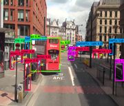
| − | In traffic scenes, usually people, traffic lights, or cars in the input image has low resolution and is small objects, while the perceptual field of the convolutional layer at the end of the YOLOv3 backbone is very large. So it is a difficult task to detect the accurate objects with YOLOv3. In computer vision tasks, invariance and equivalent transformations are two important properties in image feature representation. Classification aims to learn high-level semantic information and therefore invariant feature representations are required. The goal of object localization is to distinguish between position and scale changes, so it requires equivalence transformations. Object detection consists of two subtasks, object identification, and localization. While learning invariance and equivalence transformations are the keys to detection. The YOLOv3 is composed of a series of convolutional and pooling layers. The deep-level features have stronger invariance, but their equivalence transformation is weak. Although this is beneficial for classification recognition, it suffers from low localization accuracy in object detection. On the contrary, the shallow layer features are not conducive to semantic learning, but it contains more edge and contour information, which helps in object localization. The combination of multi-scale features can increase the global and local feature information in the model to improve the accuracy of object detection and increase the accuracy of subsequent object tracking. Therefore, to boot the detection performance of the model for small objects in traffic scenes, this paper use feature fusion technique to enhances the prediction of YOLOv3 by further integrating deep and shallow features in the model, adding a one-dimensional scale to strengthen small object prediction, and adding a residual structure in the corresponding scale branch to effectively control the gradient propagation and prevent the gradient from disappearing, degrading the network, and not easily converging, which brings about unfavorable network training. The network is easy to converge. This makes the training of the deeper network less difficult. The structure of the improved Yolov3 network is shown in Figure 3. The detail fusion process can be described as follows: | + | In traffic scenes, usually people, traffic lights, or cars in the input image has low resolution and is small objects, while the perceptual field of the convolutional layer at the end of the YOLOv3 backbone is very large. So it is a difficult task to detect the accurate objects with YOLOv3. In computer vision tasks, invariance and equivalent transformations are two important properties in image feature representation. Classification aims to learn high-level semantic information and therefore invariant feature representations are required. The goal of object localization is to distinguish between position and scale changes, so it requires equivalence transformations. Object detection consists of two subtasks, object identification, and localization. While learning invariance and equivalence transformations are the keys to detection. The YOLOv3 is composed of a series of convolutional and pooling layers. The deep-level features have stronger invariance, but their equivalence transformation is weak. Although this is beneficial for classification recognition, it suffers from low localization accuracy in object detection. On the contrary, the shallow layer features are not conducive to semantic learning, but it contains more edge and contour information, which helps in object localization. The combination of multi-scale features can increase the global and local feature information in the model to improve the accuracy of object detection and increase the accuracy of subsequent object tracking. Therefore, to boot the detection performance of the model for small objects in traffic scenes, this paper use feature fusion technique to enhances the prediction of YOLOv3 by further integrating deep and shallow features in the model, adding a one-dimensional scale to strengthen small object prediction, and adding a residual structure in the corresponding scale branch to effectively control the gradient propagation and prevent the gradient from disappearing, degrading the network, and not easily converging, which brings about unfavorable network training. The network is easy to converge. This makes the training of the deeper network less difficult. The structure of the improved Yolov3 network is shown in [[#img-3|Figure 3]]. The detail fusion process can be described as follows: |
{| class="formulaSCP" style="width: 77%;border-collapse: collapse;width: 100%;text-align: center;" | {| class="formulaSCP" style="width: 77%;border-collapse: collapse;width: 100%;text-align: center;" | ||
|- | |- | ||
| | | | ||
| − | {| style=" | + | {| style="vertical-align: top;margin:auto;width: 100%;" |
|- | |- | ||
| <math>{ffm}_{ip}={act}_{conv}\left( {act}_{FC}\left( {act}_{US}\left( {fm}_{{ir}_{high}}\right) ,\, {fm}_{{ir}_{low}}\right) \right)</math> | | <math>{ffm}_{ip}={act}_{conv}\left( {act}_{FC}\left( {act}_{US}\left( {fm}_{{ir}_{high}}\right) ,\, {fm}_{{ir}_{low}}\right) \right)</math> | ||
|} | |} | ||
| − | | style=" | + | | style="text-align: right;vertical-align: top;width: 5px;text-align: right;white-space: nowrap;"|(1) |
|} | |} | ||
| − | |||
{| class="formulaSCP" style="width: 77%;border-collapse: collapse;width: 100%;text-align: center;" | {| class="formulaSCP" style="width: 77%;border-collapse: collapse;width: 100%;text-align: center;" | ||
| Line 107: | Line 118: | ||
{| style="vertical-align: top;margin:auto;width: 100%;" | {| style="vertical-align: top;margin:auto;width: 100%;" | ||
|- | |- | ||
| − | | <math>{fm}_{ir}=\left\{ \begin{ | + | | <math>{fm}_{ir}=\left\{ \begin{array}{ll} Action\,\, ({f}_{i}),\, \, & r=0\\ |
| − | + | Action\,\, ({fm}_{ir-1}),\, \, & r=others\end{array}\right.</math> | |
| − | + | ||
|} | |} | ||
| style="text-align: right;vertical-align: top;width: 5px;text-align: right;white-space: nowrap;"|(2) | | style="text-align: right;vertical-align: top;width: 5px;text-align: right;white-space: nowrap;"|(2) | ||
|} | |} | ||
| − | |||
Where <math display="inline">{fm}_{ir}</math> indicates the r_th layer feature map of <math display="inline">{f}_{i}</math>, <math display="inline">Action</math> belongs to <math display="inline">{act}_{conv},\, {act}_{BN}\, ,\, {act}_{LR,\, }\, {act}_{Add}\, and\,</math> stands for the action of convolution, BN, ReLu and tensor addition <math display="inline">{ffm}_{ip}</math> represents the p_th fused feature map. <math display="inline">{fm}_{{ir}_{high}}</math> and <math display="inline">\, {fm}_{{ir}_{low}}</math> shows the high-resolution feature map and low-resolution feature map, respectively. <math display="inline">{act}_{US}</math> is the action of upsampling, <math display="inline">{act}_{FC}</math> is the action of full connection and <math display="inline">{act}_{conv}</math> represents the action of convolution. To describe the model later, the model is abbreviated as YOLOv3_I. | Where <math display="inline">{fm}_{ir}</math> indicates the r_th layer feature map of <math display="inline">{f}_{i}</math>, <math display="inline">Action</math> belongs to <math display="inline">{act}_{conv},\, {act}_{BN}\, ,\, {act}_{LR,\, }\, {act}_{Add}\, and\,</math> stands for the action of convolution, BN, ReLu and tensor addition <math display="inline">{ffm}_{ip}</math> represents the p_th fused feature map. <math display="inline">{fm}_{{ir}_{high}}</math> and <math display="inline">\, {fm}_{{ir}_{low}}</math> shows the high-resolution feature map and low-resolution feature map, respectively. <math display="inline">{act}_{US}</math> is the action of upsampling, <math display="inline">{act}_{FC}</math> is the action of full connection and <math display="inline">{act}_{conv}</math> represents the action of convolution. To describe the model later, the model is abbreviated as YOLOv3_I. | ||
| − | + | <div id='img-3'></div> | |
| − | + | {| class="wikitable" style="margin: 0em auto 0.1em auto;border-collapse: collapse;width:auto;" | |
| − | + | |-style="background:white;" | |
| − | + | |style="text-align: center;padding:10px;"| [[Image:Review_957358071347-image3.png|550px]] | |
| − | {| style=" | + | |
|- | |- | ||
| − | | | + | | style="background:#efefef;text-align:left;padding:10px;font-size: 85%;"| '''Figure 3'''. The structure of YOLOv3_I network |
| + | |} | ||
| − | |||
| − | |||
| + | The model is similar to YOLOv3, with only convolution layers. The size of the output feature map is controlled by adjusting the convolution step, so there is no special restriction on the input image size. Also drawing on the pyramid feature map idea, the small size feature map is applied to detect large-size objects, while the large size feature map detects small size objects. Finally, according to analysis to dataset, a total of 4 feature maps are output, the first feature map is down-sampled 32 times, the second feature map 16 times, the third 8 times, and the fourth 4 times. Four detections, each corresponding to a different field of perception, 32 down-sampling has the largest field of perception, suitable for detecting large objects, 16 for objects of average size, 8 for the smallest field of perception, suitable for prediction small objects, and even smaller objects. Considering the fact that objects have different pixels, we use different scales of anchor boxes to match. The anchor size of each cell is shown in [[#tab-1|Table 1]] according to object size of the MOT16. The whole network, which draws the essence of Resnet [27], Densenet [28], and FPN [29], incorporates the current industry effective techniques of object detection to detect the object. | ||
| − | + | <div class="center" style="font-size: 75%;">'''Table 1'''. Model anchor parameters</div> | |
| − | + | <div id='tab-1'></div> | |
| − | | | + | {| class="wikitable" style="margin: 1em auto 0.1em auto;border-collapse: collapse;font-size:85%;width:auto;" |
| − | | | + | |-style="text-align:center" |
| + | ! style="text-align:left" |Feature map !! 13*13 !! 26*26 !! 52*52 !! 104*104 | ||
|- | |- | ||
| − | | style=" | + | | style="text-align:left" | Receptive field |
| − | | style=" | + | | style="text-align: center;vertical-align: top;"|Large |
| − | | style=" | + | | style="text-align: center;vertical-align: top;"|Medium |
| − | | style=" | + | | style="text-align: center;vertical-align: top;"|Less |
| − | | style=" | + | | style="text-align: center;vertical-align: top;"|Smallest |
|- | |- | ||
| − | | style=" | + | | style="text-align: left;vertical-align: top;"|A prior box |
| + | | style="text-align: center;vertical-align: top;"| (156*198) <br> (156*198)<br> (371*326) | ||
| + | | style="text-align: center;vertical-align: top;"|(30*61) <br>(62*45)<br> (59*119) | ||
| + | | style="text-align: center;vertical-align: top;"|(10*13) <br>(16*30) <br>(33*23) | ||
| + | | style="text-align: center;vertical-align: top;"|(10*11) <br>(19*15)<br> (25*21) | ||
| + | |} | ||
| + | ===3.2. Interactive multi-model algorithms=== | ||
| − | | | + | Due to the complexity of the actual motion of the objects in the traffic scene, it is difficult to describe the motion pattern of the objects using only one model. Therefore, the algorithm in this paper adopts the Interacting Multiple Model (IMM) [30] to estimate the motion patterns of multiple objects ([[#img-4|Figure 4]]). Its main feature is the ability to approximate the state of dynamic systems with multiple patterns of behavior that can be switched from one behavior pattern to another. In particular, the IMM evaluator can be a self-tuning variable bandwidth filter, which allows it to naturally track maneuvering objects. IMM handles multi-object motion models in the Bayesian framework with a model set containing different motion sub-models, each corresponding to a filter. To solve the uncertainty of the object motion, each filter performs parallel operation computation and switches between models according to the updated weights. During object tracking, the fit of each sub-model of the system to the current object depends on the probability of the model. So, the interaction between models can be performed according to this principle, and finally the probabilistic output results of each sub-model are fused. |
| − | + | <div id='img-4'></div> | |
| − | | | + | {| class="wikitable" style="margin: 0em auto 0.1em auto;border-collapse: collapse;width:auto;" |
| − | + | |-style="background:white;" | |
| − | + | |style="text-align: center;padding:10px;"| [[File:Review 957358071347-image4.jpg|436x436px]] | |
| − | + | |- | |
| − | + | | style="background:#efefef;text-align:left;padding:10px;font-size: 85%;"| '''Figure 4'''. Flow chart of IMM algorithm | |
| − | | | + | |
| − | + | ||
| − | + | ||
| − | + | ||
| − | + | ||
| − | | | + | |
| − | + | ||
| − | + | ||
| − | + | ||
| − | + | ||
|} | |} | ||
| − | + | (1) Model initialization: <math display="inline">{M}_{k}^{j}</math> denotes the j_th filter at the k_th frame, <math display="inline">\, \, j\in \lbrace 1,\ldots ,r\rbrace</math>. | |
| − | + | ||
| − | + | ||
| − | + | ||
| − | + | ||
| − | + | ||
| − | + | ||
| − | + | ||
| − | + | ||
| − | + | ||
| − | + | ||
| − | + | ||
| − | + | ||
| − | + | ||
| − | (1) | + | |
Model initialization state <math display="inline">{\hat{X}}_{k-1\vert k-1}^{0j}</math>; Covariance matrix <math display="inline">{P}_{k-1\vert k-1}^{0j}</math>: | Model initialization state <math display="inline">{\hat{X}}_{k-1\vert k-1}^{0j}</math>; Covariance matrix <math display="inline">{P}_{k-1\vert k-1}^{0j}</math>: | ||
| Line 188: | Line 179: | ||
{| style="text-align: center; margin:auto;" | {| style="text-align: center; margin:auto;" | ||
|- | |- | ||
| − | | <math | + | | <math>{\hat{X}}_{k-1\vert k-1}^{0j}</math>= <math display="inline">\sum _{i=1}^{r}{\hat{X}}_{k-1\vert k-1}^{i}{u}_{k-1\vert k-1}^{i\vert j}</math> |
|} | |} | ||
| style="width: 5px;text-align: right;white-space: nowrap;" | (3) | | style="width: 5px;text-align: right;white-space: nowrap;" | (3) | ||
|} | |} | ||
| − | {|class="formulaSCP" style="width: 100%; text-align: | + | |
| + | {| class="formulaSCP" style="width: 100%; text-align: left;" | ||
|- | |- | ||
| − | | <math>{P}_{k-1\vert k-1}^{0j}=\sum _{i=1}^{r}{u}_{k-1\vert k-1}^{i\vert j}\left[ {P}_{k-1\vert k-1}^{j}+\left( {\hat{X}}_{k-1\vert k-1}^{i}-{\hat{X}}_{k-1\vert k-1}^{0j}\right) \times | + | | |
| + | {| style="text-align: center; margin:auto;width: 100%;" | ||
| + | |- | ||
| + | | style="text-align: center;" | <math>{P}_{k-1\vert k-1}^{0j}=\sum _{i=1}^{r}{u}_{k-1\vert k-1}^{i\vert j}\left[ {P}_{k-1\vert k-1}^{j}+\left( {\hat{X}}_{k-1\vert k-1}^{i}-{\hat{X}}_{k-1\vert k-1}^{0j}\right) \times (\hat{X}_{k-1\vert k-1-}^{i}\hat{X}_{k-1\vert k-1}^{0j})^{T}\right]</math> | ||
| + | |} | ||
| + | | style="width: 5px;text-align: right;white-space: nowrap;" |(4) | ||
|} | |} | ||
| − | + | Mixing probability <math display="inline">{u}_{k-1\vert k-1}^{i\vert j}</math>= <math display="inline">{\overline{c}}_{j}^{-1}{p}_{ij}{u}_{k-1}^{i}</math>; Normalization constants <math display="inline">{\overline{c}}_{j}=</math><math>\sum _{i=1}^{r}{p}_{ij}{u}_{k-1}^{i}</math>; <math display="inline">{p}_{ij}</math> is the Markov transition probability of filter <math> i </math> to <math> j </math>. | |
| − | + | (2) Model filtering estimation: in this paper, the standard IMM model is used, and the filtering phase has two main steps: prediction and correction. The prediction phase is responsible for calculating the a priori state estimates for each system in the current state. The correction phase is responsible for combining the actual measurements into each prior estimate to obtain the corresponding a posteriori state estimate. The motion and measurement models of the Kalman Filter are described as follows: | |
| − | + | {| class="formulaSCP" style="width: 100%; text-align: left;" | |
| − | + | ||
| − | + | ||
| − | + | ||
| − | {| class="formulaSCP" style=" | + | |
|- | |- | ||
| | | | ||
| − | {| style=" | + | {| style="text-align: center; margin:auto;width: 100%;" |
|- | |- | ||
| − | | | + | | style="text-align: center;" | <math>{\hat{X}}_{k-1\vert k-1}^{j}=A{\hat{X}}_{k-1\vert k-1}^{0j}{W}_{k}^{j}</math> |
|} | |} | ||
| − | | | + | | style="width: 5px;text-align: right;white-space: nowrap;" |(5) |
|} | |} | ||
| − | + | {| class="formulaSCP" style="width: 100%; text-align: left;" | |
| − | + | ||
| − | + | ||
| − | + | ||
| − | + | ||
| − | {| class="formulaSCP" style=" | + | |
|- | |- | ||
| | | | ||
| − | {| style=" | + | {| style="text-align: center; margin:auto;width: 100%;" |
|- | |- | ||
| − | | | + | | style="text-align: center;" | <math>{Z}_{k}^{j}=H{\hat{X}}_{k\vert k-1}^{j}+{V}_{k}^{j}</math> |
|} | |} | ||
| − | | style=" | + | | style="width: 5px;text-align: right;white-space: nowrap;" |(6) |
|} | |} | ||
| + | where <math display="inline">{\hat{X}}_{k\vert k-1\, }^{j}</math> is <math display="inline">{M}_{k}^{j}</math> a priori state estimation. <math display="inline">A, H</math> are state transition matrix, measurement matrix respectively. <math display="inline">{Z}_{k}^{j}\,</math> represents the measured value at the kth frame. <math display="inline">\, {W}_{k}^{j}</math> and <math display="inline">{V}_{k}^{j}</math> are the noise corresponding to the computational quantities obeying Gaussian distribution. Finally, the posterior state estimate is obtained | ||
| − | + | {| class="formulaSCP" style="width: 100%; text-align: left;" | |
| − | + | ||
| − | + | ||
| − | + | ||
| − | + | ||
| − | + | ||
| − | {| class="formulaSCP" style=" | + | |
|- | |- | ||
| | | | ||
| − | {| style=" | + | {| style="text-align: center; margin:auto;width: 100%;" |
|- | |- | ||
| − | | | + | | style="text-align: center;" | <math>{\hat{X}}_{k\vert k}^{j}= A{\hat{X}}_{k\vert k-1}^{j}+ {K}_{k}^{j}( {Z}_{k}^{j}-H{\hat{X}}_{k\vert k-1}^{j})</math> |
| − | + | ||
| − | + | ||
|} | |} | ||
| − | | | + | | style="width: 5px;text-align: right;white-space: nowrap;" |(7) |
|} | |} | ||
| − | |||
<math display="inline">{Z}_{k}^{j}-H{\hat{X}}_{k\vert k-1}^{j}</math> is the residual of the motion model and the measurement model. <math display="inline">{K}_{k}^{j}</math> filtering gain is defined as: | <math display="inline">{Z}_{k}^{j}-H{\hat{X}}_{k\vert k-1}^{j}</math> is the residual of the motion model and the measurement model. <math display="inline">{K}_{k}^{j}</math> filtering gain is defined as: | ||
| − | {| class="formulaSCP" style=" | + | {| class="formulaSCP" style="width: 100%; text-align: left;" |
|- | |- | ||
| | | | ||
| − | {| style=" | + | {| style="text-align: center; margin:auto;width: 100%;" |
|- | |- | ||
| − | | <math> | + | | style="text-align: center;" | <math> {K}_{k}^{j}={P}_{k-1\vert k-1}^{J}{H}^{T}{({HP}_{k\vert k-1}^{j}{H}^{T}+R)}^{-1}</math> |
| − | + | ||
| − | + | ||
|} | |} | ||
| − | | | + | | style="width: 5px;text-align: right;white-space: nowrap;" |(8) |
|} | |} | ||
| + | where the a priori covariance matrix is: | ||
| − | + | {| class="formulaSCP" style="width: 100%; text-align: left;" | |
| − | + | ||
| − | {| class="formulaSCP" style=" | + | |
|- | |- | ||
| | | | ||
| − | {| style="text-align: center | + | {| style="text-align: center; margin:auto;width: 100%;" |
|- | |- | ||
| − | | | + | | style="text-align: center;" | <math>{P}_{k\vert k-1}^{j}=A {P}_{k-1\vert k-1}^{j}{A}^{T}+Q</math> |
| − | + | ||
| − | + | ||
|} | |} | ||
| − | | | + | | style="width: 5px;text-align: right;white-space: nowrap;"|(9) |
|} | |} | ||
| Line 283: | Line 258: | ||
The posterior covariance matrix is updated as: | The posterior covariance matrix is updated as: | ||
| − | {| class="formulaSCP" style=" | + | {| class="formulaSCP" style="width: 100%; text-align: left;" |
|- | |- | ||
| | | | ||
| − | {| style=" | + | {| style="text-align: center; margin:auto;width: 100%;" |
|- | |- | ||
| − | | | + | | style="text-align: center;" | <math>{P}_{k\vert k}^{j} =(I- K_{k}^{j}H) {P}_{k\vert k-1}^{j}</math> |
|} | |} | ||
| − | | | + | | style="width: 5px;text-align: right;white-space: nowrap;"|(10) |
|} | |} | ||
| − | (3) | + | (3) Model probability updating. Calculating model probabilities: |
| − | {| class="formulaSCP" style=" | + | {| class="formulaSCP" style="width: 100%; text-align: left;" |
|- | |- | ||
| | | | ||
| − | {| style="text-align: center | + | {| style="text-align: center; margin:auto;width: 100%;" |
|- | |- | ||
| − | | | + | | style="text-align: center;" | <math>{u}_{k}^{i}=\frac{1}{c}{\Lambda }_{k}^{j}{\overline{\overline{c}}}_{j}</math> |
|} | |} | ||
| − | | | + | | style="width: 5px;text-align: right;white-space: nowrap;"|(11) |
|} | |} | ||
| − | + | {| class="formulaSCP" style="width: 100%; text-align: left;" | |
| − | {| class="formulaSCP" style=" | + | |
|- | |- | ||
| | | | ||
| − | {| style=" | + | {| style="text-align: center; margin:auto;width: 100%;" |
|- | |- | ||
| − | | <math>c=\sum _{i=1}^{r}{\Lambda }_{k}^{j}{\overline{\overline{c}}}_{i}</math> | + | | style="text-align: center;" | <math>c=\sum _{i=1}^{r}{\Lambda }_{k}^{j}{\overline{\overline{c}}}_{i}</math> |
|} | |} | ||
| − | | style=" | + | | style="width: 5px;text-align: right;white-space: nowrap;"|(12) |
|} | |} | ||
| Line 320: | Line 294: | ||
Likelihood function <math display="inline">{\Lambda }_{k}^{j}</math>: | Likelihood function <math display="inline">{\Lambda }_{k}^{j}</math>: | ||
| − | {| class="formulaSCP" style=" | + | {| class="formulaSCP" style="width: 100%; text-align: left;" |
|- | |- | ||
| | | | ||
| − | {| style="text-align: center | + | {| style="text-align: center; margin:auto;width: 100%;" |
|- | |- | ||
| − | | | + | | style="text-align: center;" | <math>{\Lambda }_{k}^{j}=N \left( {\tilde{Z}}_{k}^{j};0,\, \, {S}_{k}^{j}\, \right)</math> |
| − | + | ||
| − | + | ||
|} | |} | ||
| − | | style=" | + | | style="width: 5px;text-align: right;white-space: nowrap;"|(13) |
|} | |} | ||
| − | The filter | + | The filter residual, <math display="inline">{\tilde{Z}}_{k}^{j}= {Z}_{k}^{j}-H {\hat{X}}_{k\vert k}^{j}</math>; <math display="inline">{S}_{k}^{i}= H {P}_{k\vert k-1}^{j}{H}^{T}+R</math>, is the corresponding filtering residual matrix, and <math display="inline">N\left( \cdot \right)</math> is Gaussian distribution. If the residuals are larger, it means that the model has a larger deviation from the object localization. Its weight decreases, and vice versa, the weight increases. |
| − | (4) | + | (4) Estimated fusion. Final state estimates and their covariances: |
| − | {| class="formulaSCP" style=" | + | {| class="formulaSCP" style="width: 100%; text-align: left;" |
|- | |- | ||
| | | | ||
| − | {| style="text-align: | + | {| style="text-align: center; margin:auto;width: 100%;" |
|- | |- | ||
| − | | | + | | style="text-align: center;" | <math>{\hat{X}}_{k\vert k}^{j}= \sum _{j=1}^{r}{u}_{k}^{i}{\hat{X}}_{k\vert k}^{j}</math> |
|} | |} | ||
| − | | | + | | style="width: 5px;text-align: right;white-space: nowrap;"|(14) |
| + | |} | ||
| + | |||
| + | {| class="formulaSCP" style="width: 100%; text-align: left;" | ||
|- | |- | ||
| − | | | + | | |
| − | | style=" | + | {| style="text-align: center; margin:auto;width: 100%;" |
| + | |- | ||
| + | | style="text-align: center;" | <math>{P}_{k\vert k}= \sum _{j=1}^{r}{u}_{k}^{j}\Big[ {P}_{k\vert k}^{j}+({\hat{X}}_{k\vert k}^{j}-{\hat{X}}_{k\vert k})({\hat{X}}_{k\vert k}^{j}-{\hat{X}}_{k\vert k})^{T}\Big]</math> | ||
| + | |} | ||
| + | | style="width: 5px;text-align: right;white-space: nowrap;"|(15) | ||
|} | |} | ||
| − | |||
===3.3 Position correction optimization algorithm=== | ===3.3 Position correction optimization algorithm=== | ||
| − | In traffic scenes, traffic objects such as cars and pedestrians are usually very dense. Especially in the event of traffic congestion, the objects are easily obscured and so on. When the object is obscured, the information of the object becomes incomplete and the object is easily lost. Therefore, in the paper, a position correction algorithm that fine-tunes the tracked object position is used in order to solve the lost-following phenomenon that occurs during the object tracking. The method corrects the object position based on the original predicted position, as shown in Figure 5. When the object is not found in the tracking area predicted by the IMM [31], the algorithm firstly considers that the object has been lost. Then, two points are selected from the location predicted by the IMM and the detection area of the detection algorithm. Eight-pixel points are added around it. Next, a fixed 125 threshold is set to compare the grayscale value of each point with the object empirical grayscale value. The last, we get the best point from the ten points and determine whether the point belongs to the object position. | + | In traffic scenes, traffic objects such as cars and pedestrians are usually very dense. Especially in the event of traffic congestion, the objects are easily obscured and so on. When the object is obscured, the information of the object becomes incomplete and the object is easily lost. Therefore, in the paper, a position correction algorithm that fine-tunes the tracked object position is used in order to solve the lost-following phenomenon that occurs during the object tracking. The method corrects the object position based on the original predicted position, as shown in [[#img-5|Figure 5]]. When the object is not found in the tracking area predicted by the IMM [31], the algorithm firstly considers that the object has been lost. Then, two points are selected from the location predicted by the IMM and the detection area of the detection algorithm. Eight-pixel points are added around it. Next, a fixed 125 threshold is set to compare the grayscale value of each point with the object empirical grayscale value. The last, we get the best point from the ten points and determine whether the point belongs to the object position. |
| − | [[Image:Review_957358071347-image5.png|441x441px]] | + | <div id='img-5'></div> |
| − | + | {| class="wikitable" style="margin: 0em auto 0.1em auto;border-collapse: collapse;width:auto;" | |
| − | Figure 5. Flowchart of position correction algorithm | + | |-style="background:white;" |
| + | |style="text-align: center;padding:10px;"| [[File:Ren_et_al_2023a_6444_22-11-2023 16-16-33.png]] | ||
| + | <!--[[Image:Review_957358071347-image5.png|441x441px]]--> | ||
| + | |- | ||
| + | | style="background:#efefef;text-align:left;padding:10px;font-size: 85%;"| '''Figure 5'''. Flowchart of position correction algorithm | ||
| + | |} | ||
===3.4 Implement detail=== | ===3.4 Implement detail=== | ||
| Line 367: | Line 350: | ||
===4.1. Experiment preparation=== | ===4.1. Experiment preparation=== | ||
| − | + | The experiments are operated on the computer with Intel Core i7-7700 CPU, 3.5GHz, 8G DDR4, 2666MHz memory, and Nvidia GTX1080Ti, with Ubuntu Linux 18.04 and Python3. Deep learning framework is tensorflow. | |
The performance of the proposed detection model is proven on MOT16 and KITTI datasets. The KITTI dataset is a dataset for autonomous driving, with cars and pedestrians. The MOT16 dataset is proposed in 2016 to measure standards for multi-object tracking detection and tracking methods. The performance of the proposed multi-object tracking algorithm is evaluated on the public MOT16 dataset [32]. The MOT16 benchmark evaluates the tracking performance of challenging test sequences, including forward-looking scenes with moving cameras and top-down surveillance settings. The dataset was divided into a training set and validation set. Finally, it is compared with other multi-object tracking algorithms on the test set of MOT16. The evaluation metrics are: | The performance of the proposed detection model is proven on MOT16 and KITTI datasets. The KITTI dataset is a dataset for autonomous driving, with cars and pedestrians. The MOT16 dataset is proposed in 2016 to measure standards for multi-object tracking detection and tracking methods. The performance of the proposed multi-object tracking algorithm is evaluated on the public MOT16 dataset [32]. The MOT16 benchmark evaluates the tracking performance of challenging test sequences, including forward-looking scenes with moving cameras and top-down surveillance settings. The dataset was divided into a training set and validation set. Finally, it is compared with other multi-object tracking algorithms on the test set of MOT16. The evaluation metrics are: | ||
| − | MOTA: Multi-Object Tracking Accuracy: | + | ''MOTA: Multi-Object Tracking Accuracy'': |
{| class="formulaSCP" style="width: 77%;border-collapse: collapse;width: 100%;text-align: center;" | {| class="formulaSCP" style="width: 77%;border-collapse: collapse;width: 100%;text-align: center;" | ||
| Line 384: | Line 367: | ||
| − | GT is the number of Groundtruth. FN stands for the missing number. The number of frames t in which the object has no hypothetical position to match. FP is the number of object mismatches. The number of frames t in which the given hypothetical position has no tracking object to match it. IDs is a mismatch. The number of times the tracking object has an ID switch in frame t. | + | GT is the number of Groundtruth. FN stands for the missing number. The number of frames <math> t </math> in which the object has no hypothetical position to match. FP is the number of object mismatches. The number of frames <math> t </math> in which the given hypothetical position has no tracking object to match it. IDs is a mismatch. The number of times the tracking object has an ID switch in frame <math> t </math>. |
| − | MOTP: Multi-object tracking accuracy: | + | ''MOTP: Multi-object tracking accuracy'': |
{| class="formulaSCP" style="width: 77%;border-collapse: collapse;width: 100%;text-align: center;" | {| class="formulaSCP" style="width: 77%;border-collapse: collapse;width: 100%;text-align: center;" | ||
| Line 394: | Line 377: | ||
|- | |- | ||
| <math>MOTP=\frac{\sum _{i,j}^{}{d}_{i,j}}{\sum _{t}^{}{c}_{t}}</math> | | <math>MOTP=\frac{\sum _{i,j}^{}{d}_{i,j}}{\sum _{t}^{}{c}_{t}}</math> | ||
| − | |||
| − | |||
|} | |} | ||
| style="text-align: right;vertical-align: top;width: 5px;text-align: right;white-space: nowrap;"|(15) | | style="text-align: right;vertical-align: top;width: 5px;text-align: right;white-space: nowrap;"|(15) | ||
|} | |} | ||
| + | where <math display="inline">{c}_{t}</math> represents the number of matches between objects and hypotheses in frame <math> t </math>, and <math display="inline">{d}_{i,j}</math> denotes the distance between objects and their paired hypothesis positions in frame <math> t </math>. | ||
| − | + | ===4.2. The experiment results and analysis=== | |
| − | + | The evaluation metric of the object detection commonly contains the mean Average Precision (mAP), the Average Precision (AP), F1 score, Recall rate, and so on. The mAP is considered the average of AP of all object categories. Thus, we use mAP and F1 scores as the authoritative metric to evaluate the performance of our model. [[#tab-2|Tables 2]] and [[#tab-3|3]] | |
| + | introduce typical and related evaluation results on MOT16 and KITTI datasets. | ||
| − | < | + | <div class="center" style="font-size: 75%;">'''Table 2'''. Comparison performance of object detection model on MOT16</div> |
| − | + | <div id='tab-2'></div> | |
| − | + | {| class="wikitable" style="margin: 1em auto 0.1em auto;border-collapse: collapse;font-size:85%;width:auto;" | |
| − | {| style=" | + | |-style="text-align:center" |
| + | ! Model (Detector) !! Recall !! Precision | ||
|- | |- | ||
| − | | style=" | + | | style="text-align: center;vertical-align: top;"|FrRCNN(VGG16) |
| − | + | | style="text-align: center;vertical-align: top;"|49.5% | |
| − | + | | style="text-align: center;vertical-align: top;"|77.5% | |
| − | + | ||
| − | + | ||
| − | | style=" | + | |
| − | | style=" | + | |
|- | |- | ||
| style="text-align: center;vertical-align: top;"|FrRCNN(ZF) | | style="text-align: center;vertical-align: top;"|FrRCNN(ZF) | ||
| Line 423: | Line 403: | ||
| style="text-align: center;vertical-align: top;"|72.4% | | style="text-align: center;vertical-align: top;"|72.4% | ||
|- | |- | ||
| − | | style=" | + | | style="text-align: center;vertical-align: top;"|YOLOv3 |
| − | + | | style="text-align: center;vertical-align: top;"|48.2% | |
| − | + | | style="text-align: center;vertical-align: top;"|75.6% | |
| − | | style=" | + | |- |
| − | + | | style="text-align: center;vertical-align: top;"|YOLOv3_I | |
| − | + | | style="text-align: center;vertical-align: top;"|50.1% | |
| − | | style=" | + | | style="text-align: center;vertical-align: top;"|77.4% |
| − | + | ||
| − | 77.4% | + | |
|} | |} | ||
| − | Table 3. Comparison performance of object detection model on KITTI | + | <div class="center" style="font-size: 75%;">'''Table 3'''. Comparison performance of object detection model on KITTI</div> |
| − | {| style=" | + | <div id='tab-3'></div> |
| + | {| class="wikitable" style="margin: 1em auto 0.1em auto;border-collapse: collapse;font-size:85%;width:auto;" | ||
| + | |-style="text-align:center" | ||
| + | ! Model (Detector) !! Recall !! Precision | ||
|- | |- | ||
| − | | style=" | + | | style="text-align: center;vertical-align: top;"|FrRCNN(VGG16) |
| − | + | | style="text-align: center;vertical-align: top;"|63.9% | |
| − | + | | style="text-align: center;vertical-align: top;"|79.1% | |
| − | + | ||
| − | + | ||
| − | | style=" | + | |
| − | | style=" | + | |
|- | |- | ||
| style="text-align: center;vertical-align: top;"|FrRCNN(ZF) | | style="text-align: center;vertical-align: top;"|FrRCNN(ZF) | ||
| Line 451: | Line 428: | ||
| style="text-align: center;vertical-align: top;"|74.6% | | style="text-align: center;vertical-align: top;"|74.6% | ||
|- | |- | ||
| − | | style=" | + | | style="text-align: center;vertical-align: top;"|YOLOv3 |
| − | + | | style="text-align: center;vertical-align: top;"|75.7% | |
| − | + | | style="text-align: center;vertical-align: top;"|78.9% | |
| − | | style=" | + | |
| − | + | ||
| − | + | ||
| − | | style=" | + | |
| − | + | ||
| − | + | ||
| − | + | ||
| − | + | ||
| − | + | ||
| − | + | ||
| − | + | ||
|- | |- | ||
| − | | | + | | style="text-align: center;vertical-align: top;"|YOLOv3_I |
| − | | | + | | style="text-align: center;vertical-align: top;"|79.8% |
| + | | style="text-align: center;vertical-align: top;"|81.1% | ||
|} | |} | ||
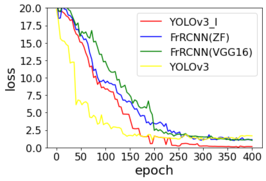
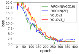
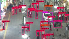
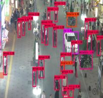
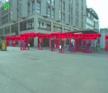
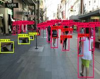
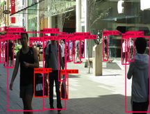
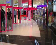
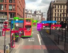
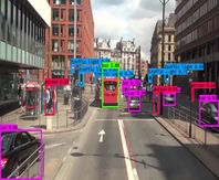
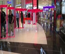
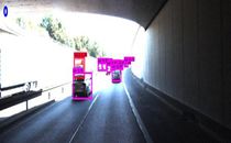
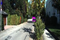
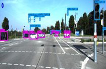
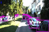
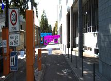
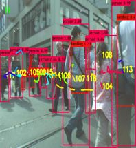
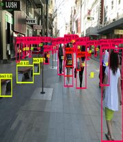
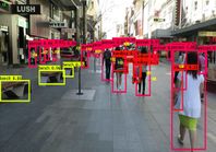
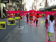
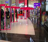
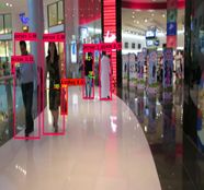
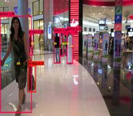
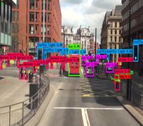
| − | + | Referring to the idea in SORT tracking algorithm, detection performance has a significant impact on tracking performance. A good detector can result in the best tracking accuracy [33]. Faster R-CNN is the popular and classical detection algorithm in the study. In this paper, we also hope to improve the tracking performance by improving the detector accuracy, as shown in [[#tab-2|Tables 2]] and [[#tab-3|3]], YOLOv3_I outperforms Faster R-CNN in terms of object detection effect and has more advantages in detection speed and accuracy, which is more beneficial to have better behavior of multi-object tracking. In the process of pedestrian detection, the paper uses the parameters obtained from training in PASCAL VOC for initialization. The table compares two network architectures provided by FrRCNN, namely Zeiler and Fergus' architecture (FrRCNN(ZF)) [34] Simonyan and Zisserman's deeper architecture (FrRCNN(VGG16)) [35] and the paper's improved multi-scale fusion model based on YOLOv3, named YOLOv3_I which shows that the model used in this paper obtains better detection recall and accuracy. It can be facilitated the later object tracking. [[#img-6|Figure 6]] gives detection result of epoch vs loss on MOT16 and KITTI datasets. The proposed model compared with other models has good convergence speed. [[#img-7|Figures 7]] and [[#img-8|8]] show the schematic diagrams of the detection output of the YOLOv3_I model, in which the corresponding confidence, classification, and localization are given for the detected objects. In the final tracking part of the experiments, only the objects with the detection probability confidence greater than 50% are passed to tracking model in the paper. | |
| − | + | <div id='img-6'></div> | |
| − | {| | + | {| class="wikitable" style="margin: 0em auto 0.1em auto;border-collapse: collapse;width:auto;" |
| + | |-style="background:white;" | ||
| + | |align="center" | | ||
| + | {|style="margin: 0em auto 0.1em auto;width:auto;" | ||
| + | |+ | ||
|- | |- | ||
| − | | [[Image:Review_957358071347- | + | |style="text-align: center;padding:10px;"| [[Image:Review_957358071347-image6.png|266px]] |
| − | | [[Image:Review_957358071347- | + | | style="text-align: center;padding:10px;"|[[Image:Review_957358071347-image7.png|center|266px]] |
|} | |} | ||
| − | |||
| − | |||
| − | |||
| − | |||
|- | |- | ||
| − | | | + | | style="background:#efefef;text-align:left;padding:10px;font-size: 85%;"| '''Figure 6'''. YOLOv3_I detection epoch vs loss on MOT16 (left) and KITTI (right) |
| − | + | ||
|} | |} | ||
| − | + | <div id='img-7'></div> | |
| − | {| | + | {| class="wikitable" style="margin: 0em auto 0.1em auto;border-collapse: collapse;width:auto;" |
| + | |-style="background:white;" | ||
| + | |align="center" | | ||
| + | {|style="margin: 0em auto 0.1em auto;width:auto;" | ||
| + | |+ | ||
|- | |- | ||
| − | | [[Image:Review_957358071347- | + | |style="text-align: center;padding:10px;"| [[Image:Review_957358071347-image8.jpeg|236px]] |
| − | | [[Image:Review_957358071347- | + | | style="text-align: center;padding:10px;"| [[Image:Review_957358071347-image9.jpeg|center|204px]] |
| − | + | ||
| − | + | ||
| − | + | ||
| − | + | ||
| − | + | ||
|- | |- | ||
| − | | [[Image:Review_957358071347- | + | |style="text-align: center;padding:10px;"|[[Image:Review_957358071347-image10.jpeg|216px]] |
| − | | [[Image:Review_957358071347- | + | |style="text-align: center;padding:10px;"| [[Image:Review_957358071347-image11.jpeg|center|198px]] |
| − | | | + | |- |
| − | + | |style="text-align: center;padding:10px;"|[[Image:Review_957358071347-image12.jpeg|216px]] | |
| − | + | |style="text-align: center;padding:10px;"|[[Image:Review_957358071347-image13.jpeg|center|198px]] | |
| − | + | ||
| − | + | ||
| − | + | ||
| − | + | ||
|- | |- | ||
| − | | [[Image:Review_957358071347- | + | |style="text-align: center;padding:10px;"|[[Image:Review_957358071347-image14.jpeg|216px]] |
| − | | [[Image:Review_957358071347- | + | | style="text-align: center;padding:10px;"|[[Image:Review_957358071347-image15.jpeg|center|198px]] |
|} | |} | ||
| − | |||
| − | |||
| − | |||
| − | |||
|- | |- | ||
| − | | | + | | style="background:#efefef;text-align:left;padding:10px;font-size: 85%;"| '''Figure 7'''. YOLOv3_I detection results schematic diagram on MOT16 |
| − | + | ||
|} | |} | ||
| − | + | <div id='img-8'></div> | |
| − | {| | + | {| class="wikitable" style="margin: 0em auto 0.1em auto;border-collapse: collapse;width:auto;" |
| + | |-style="background:white;" | ||
| + | |align="center" | | ||
| + | {|style="margin: 0em auto 0.1em auto;width:auto;" | ||
| + | |+ | ||
| + | |- | ||
| + | |style="text-align: center;padding:10px;"| [[Image:Review_957358071347-image16.jpeg|216px]] | ||
| + | | style="text-align: center;padding:10px;"| [[Image:Review_957358071347-image17.jpeg|center|198px]] | ||
|- | |- | ||
| − | | [[Image:Review_957358071347-image20.jpeg|210px]] | + | |style="text-align: center;padding:10px;"|[[Image:Review_957358071347-image18.jpeg|210px]] |
| − | | [[Image:Review_957358071347-image21.jpeg|center|210px]] | + | |style="text-align: center;padding:10px;"| [[Image:Review_957358071347-image19.jpeg|center|204px]] |
| + | |- | ||
| + | |style="text-align: center;padding:10px;"|[[Image:Review_957358071347-image20.jpeg|210px]] | ||
| + | |style="text-align: center;padding:10px;"|[[Image:Review_957358071347-image21.jpeg|center|210px]] | ||
| + | |- | ||
| + | |style="text-align: center;padding:10px;"|[[Image:Review_957358071347-image22.jpeg|216px]] | ||
| + | | style="text-align: center;padding:10px;"|[[Image:Review_957358071347-image23.jpeg|center|204px]] | ||
|} | |} | ||
| − | |||
| − | |||
| − | |||
| − | |||
|- | |- | ||
| − | | | + | | style="background:#efefef;text-align:left;padding:10px;font-size: 85%;"| '''Figure 8'''. YOLOv3_I detection results schematic diagram on KITTI |
| − | + | ||
|} | |} | ||
| − | |||
| − | |||
| − | |||
| − | |||
| − | |||
===4.3. Analysis of experimental results of multi-object tracking model=== | ===4.3. Analysis of experimental results of multi-object tracking model=== | ||
| − | The proposed method is compared with several existing object tracking methods on the MOT2016 to test the various performances of the algorithm, as shown in Table 4. All benchmark testing methods and our approach use the same publicly available test results for a fair comparison. The proposed method outperforms previous approaches in terms of MOTP, ML, and Frag. The offline tracking method can access all future detection results and reason on the data association step, and the results show that the MOTP of the proposed method is better than that of the offline method with about 3 percentage point higher performance. The technique using object correction can find the correct object after occlusion or drift. Therefore, our experiment results have higher MT and lower ML, but the IDS is higher. When the objects are occluded, the proposed method in the paper may incorrectly assign them to other detection objects. However, when the objects reappear, the methods proposed will re-match them with the correct detection results. Such a process can lead to a large number of switches. But the Frag metric is still high. | + | The proposed method is compared with several existing object tracking methods on the MOT2016 to test the various performances of the algorithm, as shown in [[#tab-4|Table 4]]. All benchmark testing methods and our approach use the same publicly available test results for a fair comparison. The proposed method outperforms previous approaches in terms of MOTP, ML, and Frag. The offline tracking method can access all future detection results and reason on the data association step, and the results show that the MOTP of the proposed method is better than that of the offline method with about 3 percentage point higher performance. The technique using object correction can find the correct object after occlusion or drift. Therefore, our experiment results have higher MT and lower ML, but the IDS is higher. When the objects are occluded, the proposed method in the paper may incorrectly assign them to other detection objects. However, when the objects reappear, the methods proposed will re-match them with the correct detection results. Such a process can lead to a large number of switches. But the Frag metric is still high. |
| − | + | <div class="center" style="font-size: 75%;">'''Table 4'''. Benchmark tracking performance comparison on MOT16</div> | |
| − | + | <div id='tab-4'></div> | |
| − | + | {| class="wikitable" style="margin: 1em auto 0.1em auto;border-collapse: collapse;font-size:85%;width:auto;" | |
| − | {| style=" | + | |-style="text-align:center" |
| + | ! Method !! Mode !! MOTA↑ !!MOTP↑ !! MT↑ !! ML↓ !! IDs↓ !! Frag↓ | ||
|- | |- | ||
| − | | style=" | + | | style="text-align: center;vertical-align: top;"|MCjoint [36] |
| − | + | | style="text-align: center;vertical-align: top;"|Offline | |
| − | + | | style="text-align: center;vertical-align: top;"|47.1 | |
| − | + | | style="text-align: center;vertical-align: top;"|76.3 | |
| − | + | | style="text-align: center;vertical-align: top;"|20.4 | |
| − | + | | style="text-align: center;vertical-align: top;"|46.9 | |
| − | + | | style="text-align: center;vertical-align: top;"|370 | |
| − | + | | style="text-align: center;vertical-align: top;"|598 | |
| − | + | ||
| − | + | ||
| − | | style=" | + | |
| − | | style=" | + | |
| − | | style=" | + | |
| − | | style=" | + | |
| − | | style=" | + | |
| − | | style=" | + | |
| − | | style=" | + | |
|- | |- | ||
| − | | style="text-align: center;vertical-align: top;"|SMOT[37] | + | | style="text-align: center;vertical-align: top;"|SMOT [37] |
| style="text-align: center;vertical-align: top;"|Offline | | style="text-align: center;vertical-align: top;"|Offline | ||
| style="text-align: center;vertical-align: top;"|29.7 | | style="text-align: center;vertical-align: top;"|29.7 | ||
| Line 580: | Line 531: | ||
| style="text-align: center;vertical-align: top;"|4483 | | style="text-align: center;vertical-align: top;"|4483 | ||
|- | |- | ||
| − | | style="text-align: center;vertical-align: top;"|NOMT[19] | + | | style="text-align: center;vertical-align: top;"|NOMT [19] |
| style="text-align: center;vertical-align: top;"|Offline | | style="text-align: center;vertical-align: top;"|Offline | ||
| style="text-align: center;vertical-align: top;"|46.4 | | style="text-align: center;vertical-align: top;"|46.4 | ||
| Line 589: | Line 540: | ||
| style="text-align: center;vertical-align: top;"|504 | | style="text-align: center;vertical-align: top;"|504 | ||
|- | |- | ||
| − | | style="text-align: center;vertical-align: top;"|LMP[38] | + | | style="text-align: center;vertical-align: top;"|LMP [38] |
| style="text-align: center;vertical-align: top;"|Offline | | style="text-align: center;vertical-align: top;"|Offline | ||
| style="text-align: center;vertical-align: top;"|48.8 | | style="text-align: center;vertical-align: top;"|48.8 | ||
| Line 598: | Line 549: | ||
| style="text-align: center;vertical-align: top;"|595 | | style="text-align: center;vertical-align: top;"|595 | ||
|- | |- | ||
| − | | style="text-align: center;vertical-align: top;"|OVBT[39] | + | | style="text-align: center;vertical-align: top;"|OVBT [39] |
| style="text-align: center;vertical-align: top;"|Online | | style="text-align: center;vertical-align: top;"|Online | ||
| style="text-align: center;vertical-align: top;"|38.4 | | style="text-align: center;vertical-align: top;"|38.4 | ||
| Line 607: | Line 558: | ||
| style="text-align: center;vertical-align: top;"|2140 | | style="text-align: center;vertical-align: top;"|2140 | ||
|- | |- | ||
| − | | style="text-align: center;vertical-align: top;"|EAMTT[40] | + | | style="text-align: center;vertical-align: top;"|EAMTT [40] |
| style="text-align: center;vertical-align: top;"|Online | | style="text-align: center;vertical-align: top;"|Online | ||
| style="text-align: center;vertical-align: top;"|38.8 | | style="text-align: center;vertical-align: top;"|38.8 | ||
| Line 616: | Line 567: | ||
| style="text-align: center;vertical-align: top;"|1657 | | style="text-align: center;vertical-align: top;"|1657 | ||
|- | |- | ||
| − | | style="text-align: center;vertical-align: top;"|oICF[41] | + | | style="text-align: center;vertical-align: top;"|oICF [41] |
| style="text-align: center;vertical-align: top;"|Online | | style="text-align: center;vertical-align: top;"|Online | ||
| style="text-align: center;vertical-align: top;"|43.2 | | style="text-align: center;vertical-align: top;"|43.2 | ||
| Line 625: | Line 576: | ||
| style="text-align: center;vertical-align: top;"|1404 | | style="text-align: center;vertical-align: top;"|1404 | ||
|- | |- | ||
| − | | style="text-align: center;vertical-align: top;"|SORT[33] | + | | style="text-align: center;vertical-align: top;"|SORT [33] |
| style="text-align: center;vertical-align: top;"|Online | | style="text-align: center;vertical-align: top;"|Online | ||
| style="text-align: center;vertical-align: top;"|59.8 | | style="text-align: center;vertical-align: top;"|59.8 | ||
| Line 634: | Line 585: | ||
| style="text-align: center;vertical-align: top;"|1664 | | style="text-align: center;vertical-align: top;"|1664 | ||
|- | |- | ||
| − | | style="text-align: center;vertical-align: top;"|Deep SORT[42] | + | | style="text-align: center;vertical-align: top;"|Deep SORT [42] |
| style="text-align: center;vertical-align: top;"|Online | | style="text-align: center;vertical-align: top;"|Online | ||
| style="text-align: center;vertical-align: top;"|61.4 | | style="text-align: center;vertical-align: top;"|61.4 | ||
| Line 643: | Line 594: | ||
| style="text-align: center;vertical-align: top;"|1023 | | style="text-align: center;vertical-align: top;"|1023 | ||
|- | |- | ||
| − | | style=" | + | | style="text-align: center;vertical-align: top;"|Our |
| − | | style=" | + | | style="text-align: center;vertical-align: top;"|Online |
| − | | style=" | + | | style="text-align: center;vertical-align: top;"|61.7 |
| − | | style=" | + | | style="text-align: center;vertical-align: top;"|80.6 |
| − | | style=" | + | | style="text-align: center;vertical-align: top;"|23.5 |
| − | | style=" | + | | style="text-align: center;vertical-align: top;"|16.3 |
| − | | style=" | + | | style="text-align: center;vertical-align: top;"|837 |
| − | | style=" | + | | style="text-align: center;vertical-align: top;"|1705 |
|} | |} | ||
| − | + | The red boxes represent the person and give confidence for the corresponding objects. The red indicates the result of pedestrian tracking. The yellow numbers give the ID of the pedestrian tracking in [[#img-9|Figure 9]] (only the pedestrian ID is given because the objects are too dense). In this figure, cars or pedestrians move from far to near or near to far, showing the same class or the scale size of object change over time, which reflects the different scale changes of the object. Correspondingly, YOLOv3_I uses 4 scale features for fusion to obtain detection results in feature maps of different depths. Smaller objects can be detected in larger feature maps, while larger objects can be examined in relatively smaller feature maps, which can the detection objects at different scales. | |
| − | + | <div id='img-9'></div> | |
| − | {| | + | {| class="wikitable" style="margin: 0em auto 0.1em auto;border-collapse: collapse;width:auto;" |
| + | |-style="background:white;" | ||
| + | |align="center" | | ||
| + | {|style="margin: 0em auto 0.1em auto;width:auto;" | ||
| + | |+ | ||
|- | |- | ||
| − | | [[Image:Review_957358071347-image24.jpeg|192px]] | + | |style="text-align: center;padding:10px;"| [[Image:Review_957358071347-image24.jpeg|192px]] |
| − | | [[Image:Review_957358071347-image25.jpeg|center|186px]] | + | |style="text-align: center;padding:10px;"| [[Image:Review_957358071347-image25.jpeg|center|186px]] |
| − | |[[Image:Review_957358071347-image26.jpeg|204px]] | + | |style="text-align: center;padding:10px;"|[[Image:Review_957358071347-image26.jpeg|204px]] |
| − | + | ||
| − | + | ||
| − | + | ||
| − | + | ||
| − | + | ||
| − | + | ||
| − | + | ||
|- | |- | ||
| − | | | + | |colspan="3" style="text-align: center;font-size: 75%;padding-bottom:10px;"|(a) On MOT16-01 |
| − | + | ||
| − | + | ||
| − | + | ||
| − | + | ||
| − | + | ||
| − | ( | + | |
| − | + | ||
| − | + | ||
| − | + | ||
|- | |- | ||
| − | | [[Image:Review_957358071347- | + | |style="text-align: center;padding:10px;"| [[Image:Review_957358071347-image27.jpeg|186px]] |
| − | | | + | |style="text-align: center;padding:10px;"| [[Image:Review_957358071347-image28.jpeg|center|192px]] |
| − | |[[Image:Review_957358071347- | + | |style="text-align: center;padding:10px;"|[[Image:Review_957358071347-image29.jpeg|198px]] |
| − | | | + | |
| − | + | ||
| − | + | ||
| − | + | ||
| − | + | ||
| − | + | ||
| − | + | ||
|- | |- | ||
| − | | | + | |colspan="3" style="text-align: center;font-size: 75%;padding-bottom:10px;"|(b) On MOT16-03 |
| − | + | ||
| − | + | ||
| − | + | ||
| − | + | ||
| − | + | ||
| − | ( | + | |
| − | + | ||
| − | + | ||
| − | + | ||
|- | |- | ||
| − | | [[Image:Review_957358071347- | + | |style="text-align: center;padding:10px;"| [[Image:Review_957358071347-image30.jpeg|190px]] |
| − | | [[Image:Review_957358071347- | + | |style="text-align: center;padding:10px;"| [[Image:Review_957358071347-image31.jpeg|center|198px]] |
| − | |[[Image:Review_957358071347- | + | |style="text-align: center;padding:10px;"|[[Image:Review_957358071347-image32.jpeg|198px]] |
| − | | | + | |- |
| − | + | |colspan="3" style="text-align: center;font-size: 75%;padding-bottom:10px;"|(c) On MOT16-06 | |
| − | + | |- | |
| − | ( | + | |style="text-align: center;padding:10px;"| [[Image:Review_957358071347-image33.jpeg|180px]] |
| − | + | |style="text-align: center;padding:10px;"| [[Image:Review_957358071347-image34.jpeg|center|198px]] | |
| − | + | |style="text-align: center;padding:10px;"|[[Image:Review_957358071347-image35.jpeg|192px]] | |
| − | + | ||
|- | |- | ||
| − | | [[Image:Review_957358071347-image39.jpeg|192px]] | + | |colspan="3" style="text-align: center;font-size: 75%;padding-bottom:10px;"|(d) On MOT16-07 |
| − | | [[Image:Review_957358071347-image40.jpeg|center|192px]] | + | |- |
| − | |[[Image:Review_957358071347-image41.jpeg|186px]] | + | |style="text-align: center;padding:10px;"| [[Image:Review_957358071347-image36.jpeg|186px]] |
| + | |style="text-align: center;padding:10px;"| [[Image:Review_957358071347-image37.jpeg|center|198px]] | ||
| + | |style="text-align: center;padding:10px;"|[[Image:Review_957358071347-image38.jpeg|180px]] | ||
| + | |- | ||
| + | |colspan="3" style="text-align: center;font-size: 75%;padding-bottom:10px;"|(e) On MOT16-08 | ||
| + | |- | ||
| + | |style="text-align: center;padding:10px;"| [[Image:Review_957358071347-image39.jpeg|192px]] | ||
| + | |style="text-align: center;padding:10px;"| [[Image:Review_957358071347-image40.jpeg|center|192px]] | ||
| + | |style="text-align: center;padding:10px;"|[[Image:Review_957358071347-image41.jpeg|186px]] | ||
| + | |- | ||
| + | |colspan="3" style="text-align: center;font-size: 75%;padding-bottom:10px;"|(f) On MOT16-12 | ||
| + | |- | ||
| + | |style="text-align: center;padding:10px;"| [[Image:Review_957358071347-image42.jpeg|192px]] | ||
| + | |style="text-align: center;padding:10px;"| [[Image:Review_957358071347-image43.jpeg|center|204px]] | ||
| + | |style="text-align: center;padding:10px;"| [[Image:Review_957358071347-image44.jpeg|180px]] | ||
| + | |- | ||
| + | |colspan="3" style="text-align: center;font-size: 75%;padding-bottom:10px;"|(g) On MOT16-14 | ||
|} | |} | ||
| − | |||
| − | |||
| − | |||
| − | |||
| − | |||
| − | |||
|- | |- | ||
| − | | | + | | style="background:#efefef;text-align:left;padding:10px;font-size: 85%;"| '''Figure 9'''. Results of our method on MOT16 (a,b,c,d,e,f,g) |
| − | + | ||
| − | + | ||
|} | |} | ||
| − | |||
| − | |||
| − | |||
| − | |||
| − | |||
==5. Conclusion== | ==5. Conclusion== | ||
| Line 742: | Line 667: | ||
'''Author Contributions: '''Conceptualization, C.R., H. Y., and W. L; Data curation, G.Z. and H. Y.; Formal analysis, C.R.; Funding acquisition, G.Z.; Investigation, G. Z., K. Z., H. Y. and S. Z.; Methodology, C.R., K. Z., S. Z. and W.L.; Project administration, G. Z.; Resources, G. Z., K. Z., H. Y.and S. Z.; Software, C. R. and W. L.; Validation, G. Z.; Visualization, K. Z. and S. Z.; Writing – original draft, C. R.; Writing – review & editing, K. Z. All authors have read and agreed to the published version of the manuscript. | '''Author Contributions: '''Conceptualization, C.R., H. Y., and W. L; Data curation, G.Z. and H. Y.; Formal analysis, C.R.; Funding acquisition, G.Z.; Investigation, G. Z., K. Z., H. Y. and S. Z.; Methodology, C.R., K. Z., S. Z. and W.L.; Project administration, G. Z.; Resources, G. Z., K. Z., H. Y.and S. Z.; Software, C. R. and W. L.; Validation, G. Z.; Visualization, K. Z. and S. Z.; Writing – original draft, C. R.; Writing – review & editing, K. Z. All authors have read and agreed to the published version of the manuscript. | ||
| − | + | <!--'''Institutional Review Board Statement: '''Not applicable. | |
| − | '''Institutional Review Board Statement: '''Not applicable. | + | |
'''Informed Consent Statement: '''Not applicable. | '''Informed Consent Statement: '''Not applicable. | ||
| − | '''Data Availability Statement: '''Not applicable. | + | '''Data Availability Statement: '''Not applicable.--> |
'''Conflicts of Interest: '''The authors declare no conflict of interest. | '''Conflicts of Interest: '''The authors declare no conflict of interest. | ||
| Line 755: | Line 679: | ||
The following abbreviations are used in this manuscript: | The following abbreviations are used in this manuscript: | ||
| − | {| style="width: | + | {| style="width: 40%;" |
|- | |- | ||
| − | | <span style="text-align: center; font-size: | + | | <span style="text-align: center; font-size: 85%;">IMM:</span> |
| − | | <span style="text-align: center; font-size: | + | | <span style="text-align: center; font-size: 85%;">Interacting Multiple Model</span> |
|- | |- | ||
| − | | <span style="text-align: center; font-size: | + | | <span style="text-align: center; font-size: 85%;">YOLOv3:</span> |
| − | | <span style="text-align: center; font-size: | + | | <span style="text-align: center; font-size: 85%;">You Only Look Once Version3</span> |
|- | |- | ||
| − | | <span style="text-align: center; font-size: | + | | <span style="text-align: center; font-size: 85%;">SVM:</span> |
| − | | <span style="text-align: center; font-size: | + | | <span style="text-align: center; font-size: 85%;">Support Vector Machines</span> |
|- | |- | ||
| − | | <span style="text-align: center; font-size: | + | | <span style="text-align: center; font-size: 85%;">RPN:</span> |
| − | | <span style="text-align: center; font-size: | + | | <span style="text-align: center; font-size: 85%;">Region Proposal Network</span> |
|- | |- | ||
| − | | <span style="text-align: center; font-size: | + | | <span style="text-align: center; font-size: 85%;">ITS:</span> |
| − | | <span style="text-align: center; font-size: | + | | <span style="text-align: center; font-size: 85%;">Intelligent Transportation System</span> |
|- | |- | ||
| − | | <span style="text-align: center; font-size: | + | | <span style="text-align: center; font-size: 85%;">FP:</span> |
| − | | <span style="text-align: center; font-size: | + | | <span style="text-align: center; font-size: 85%;">False Positive</span> |
|- | |- | ||
| − | | <span style="text-align: center; font-size: | + | | <span style="text-align: center; font-size: 85%;">FN:</span> |
| − | | <span style="text-align: center; font-size: | + | | <span style="text-align: center; font-size: 85%;">False Negative</span> |
|- | |- | ||
| − | | <span style="text-align: center; font-size: | + | | <span style="text-align: center; font-size: 85%;">CNN:</span> |
| − | | <span style="text-align: center; font-size: | + | | <span style="text-align: center; font-size: 85%;">Convolutional Neural Network</span> |
|- | |- | ||
| − | | <span style="text-align: center; font-size: | + | | <span style="text-align: center; font-size: 85%;">RoI:</span> |
| − | | <span style="text-align: center; font-size: | + | | <span style="text-align: center; font-size: 85%;">Region of Interest </span> |
|} | |} | ||
| − | |||
==References== | ==References== | ||
| − | 1 | + | <div class="auto" style="text-align: left;width: auto; margin-left: auto; margin-right: auto;font-size: 85%;"> |
| + | |||
| + | [1] Xu Y., Zhou X., Chen S., Li F. Deep learning for multiple object tracking: a survey. IET Computer Vision, 13(4):355-368, 2019. | ||
| − | 2 | + | [2] Ciaparrone G., Sánchez F.L., Tabik S., Troiano L., Tagliaferri R., Herrera F. Deep learning in video multi-object tracking: A survey. Neurocomputing, 381:61-88, 2020. |
| − | 3 | + | [3] Li X., Wang K., Wang W., Li Y. A multiple object tracking method using Kalman filter. The 2010 IEEE international conference on information and automation, IEEE, pp. 1862-1866, 2010. |
| − | 4 | + | [4] Henriques J.F., Caseiro R., Martins P., Batista J. High-speed tracking with kernelized correlation filters. IEEE Transactions on Pattern Analysis and Machine Intelligence, 37(3):583-596, 2014. |
| − | 5 | + | [5] Li X., Hu W., Shen C., Zhang Z., Dick A., Hengel A. A survey of appearance models in visual object tracking. ACM transactions on Intelligent Systems and Technology (TIST), 4(4):1-48, 2013. |
| − | 6 | + | [6] LeCun Y., Bengio Y., Hinton G. Deep learning. Nature, 521:436-444, 2015. |
| − | 7 | + | [7] Yu F., Li W., Li Q., Liu Y., Shi X., Yan J. POI: multiple object tracking with high performance detection and appearance feature. European Conference on Computer Vision, Springer International Publishing, pp. 36-42, 2016. |
| − | 8 | + | [8] Zhang L., Gray H., Ye X., Collins L., Allinson N. Automatic individual pig detection and tracking in pig farms. Sensors, 19(5):1188, 2019. |
| − | 9 | + | [9] Zhao D., Fu H., Xiao L., Wu T., Dai B. Multi-object tracking with correlation filter for autonomous vehicle. Sensors, 18(7):2004, 2018. |
| − | 10 | + | [10] Wang Y., Wei X., Tang X., Shen H., Zhang H. Adaptive fusion CNN features for RGBT object tracking. IEEE Transactions on Intelligent Transportation Systems, 23(7):7831-7840, 2022. |
| − | 11 | + | [11] Xie Y., Shen J., Wu C. Affine geometrical region CNN for object tracking. IEEE Access, 8:68638-68648, 2020. |
| − | 12 | + | [12] Chintalacheruvu N., Muthukumar V. Video based vehicle detection and its application in intelligent transportation systems. Journal of Transportation Technologies, 2(04):305, 2012. |
| − | 13 | + | [13] Hinz G., Chen G., Aafaque M., Röhrbein F., Conradt J., Bing Z., Qu Z., Stechele W., Knoll A. Online multi-object tracking-by-clustering for intelligent transportation system with neuromorphic vision sensor. Joint German/Austrian Conference on Artificial Intelligence (Künstliche Intelligenz), Springer, pp. 142-154, 2017. |
| − | 14 | + | [14] Liang H., Song H., Li H., Dai Z. Vehicle counting system using deep learning and multi-object tracking methods. Transportation Research Record, 2674(4):114-128, 2020. |
| − | 15 | + | [15] Pino I. del, Vaquero V., Masini B.v Sola J., Moreno-Noguer F., Sanfeliu A., Andrade-Cetto J. Low resolution lidar-based multi-object tracking for driving applications. Iberian Robotics Conference, Springe, pp. 287-298, 2017. |
| − | 16 | + | [16] Liu Y., Li X., Bai T., Wang K., Wang F.Y. Multi-object tracking with hard-soft attention network and group-based cost minimization. Neurocomputing, 447:80-91, 2021. |
| − | 17 | + | [17] Abbas Q. V-ITS: Video-based intelligent transportation system for monitoring vehicle illegal activities. Int. J. Adv. Comput. Sci. Appl., 10(3):202-208, 2019. |
| − | 18 | + | [18] Dirir A., Adib M., Mahmoud A., Al-Gunaid M., El-Sayed H. An efficient multi-object tracking and counting framework using video streaming in urban vehicular environments. 2020 International Conference on Communications, Signal Processing, and their Applications (ICCSPA), IEEE, pp. 1-7, 2021. |
| − | 19 | + | [19] Nizar T.N., Anbarsanti N., Prihatmanto A.S. Multi-object tracking and detection system based on feature detection of the intelligent transportation system. 2014 IEEE 4th International Conference on System Engineering and Technology (ICSET), IEEE, pp. 1-6, 2014. |
| − | 20 | + | [20] Tian W., Lauer M., Chen L. Online multi-object tracking using joint domain information in traffic scenarios. IEEE Transactions on Intelligent Transportation Systems, 21(1):374-384, 2020. |
| − | 21 | + | [21] Rangesh A., Trivedi M.M. No blind spots: Full-surround multi-object tracking for autonomous vehicles using cameras and lidars. IEEE Transactions on Intelligent Vehicles, 4(4):588-599, 2019. |
| − | 22 | + | [22] Vasic M., Martinoli A. A collaborative sensor fusion algorithm for multi-object tracking using a Gaussian mixture probability hypothesis density filter. 2015 IEEE 18th International Conference on Intelligent Transportation Systems, IEEE, pp. 491-498, 2015. |
| − | 23 | + | [23] Emami P., Elefteriadou L., Ranka S. Long-range multi-object tracking at traffic intersections on low-power devices. IEEE Transactions on Intelligent Transportation Systems, 23(3):2482-2493, 2022. |
| − | 24 | + | [24] Gómez–Huélamo C., Bergasa L.M., Gutiérrez R., Arango J.F., Díaz A. SmartMOT: Exploiting the fusion of HDMaps and multi-object tracking for real-time scene understanding in intelligent vehicles applications. 2021 IEEE Intelligent Vehicles Symposium (IV), IEEE, Nagoya, Japan, pp. 710-715, 2021. |
| − | 25 | + | [25] Redmon J., Farhadi A. Yolov3: An incremental improvement. arXiv preprint arXiv:1804.02767, 2018. |
| − | 26 | + | [26] Faure F., Duriez C., Delingette H., Allard J., Gilles B., Marchesseau S., Talbot H., Courtecuisse H., Bousquet G., Peterlik I. Sofa: A multi-model framework for interactive physical simulation. Soft Tissue Biomechanical Modeling for Computer Assisted Surgery, Springer, vol. 11, 283-321, 2012. |
| − | 27 | + | [27] Wu Z., Shen C., Hengel A. Wider or deeper: Revisiting the resnet model for visual recognition. Pattern Recognition, 90:119-133, 2019. |
| − | 28 | + | [28] Iandola F., Moskewicz M., Karayev S., Girshick R., Darrell T., Keutzer K. Densenet: Implementing efficient convnet descriptor pyramids. arXiv preprint arXiv:1404.1869, 2014. |
| − | 29 | + | [29] Ghiasi G., Lin T.-Y., Le Q.V. Nas-fpn: Learning scalable feature pyramid architecture for object detection. Proceedings of the IEEE/CVF Conference on Computer Vision and Pattern Recognition, Long Beach, CA, USA, pp. 7029-7038, 2019. |
| − | 30 | + | [30] He R., Lee W.S., Ng H.T., Dahlmeier D. An interactive multi-task learning network for end-to-end aspect-based sentiment analysis. arXiv preprint arXiv:1906.06906, 2019. |
| − | 31 | + | [31] Welch G.F. Kalman filter. Computer vision: A reference guide, Springer, Cham, pp. 721-723, 2021. |
| − | 32 | + | [32] Dendorfer P., Rezatofighi H., Milan A., Shi J., Cremers D., Reid I., Roth S., Schindler K., Leal-Taixé L. Mot20: A benchmark for multi object tracking in crowded scenes. arXiv preprint arXiv:2003.09003, 2020. |
| − | 33 | + | [33] Fu H., Wu L., Jian M., Yang Y., Wang X., MF-SORT: Simple online and realtime tracking with motion features. International Conference on Image and Graphics, Springer, pp. 157-168, 2019. |
| − | 34 | + | [34] Zeiler M., Fergus R. Visualizing and understanding convolutional networks. arXiv 2013. 2019. |
| − | 35 | + | [35] Simonyan K., Zisserman A. Very deep convolutional networks for large-scale image recognition. arXiv preprint arXiv:1409.1556, 2018. |
| − | 36 | + | [36] Keuper M., Tang S., Zhongjie Y., Andres B., Brox T., Schiele B. A multi-cut formulation for joint segmentation and tracking of multiple objects. arXiv preprint arXiv:1607.06317, 2016. |
| − | 37 | + | [37] Choi W. Near-online multi-object tracking with aggregated local flow descriptor. 2015 IEEE Proceedings of the International Conference on Computer Vision, pp. 3029-3037, 2015. |
| − | 38 | + | [38] Tang S., Andriluka M., Andres B., Schiele B. Multiple people tracking by lifted multicut and person re-identification. 2017 IEEE Conference on Computer Vision and Pattern Recognition, pp. 3701-3710, 2017. |
| − | 39 | + | [39] Ban Y., Ba S., Alameda-Pineda X., Horaud R. Tracking multiple persons based on a variational Bayesian model. European Conference on Computer Vision – ECCV 2016 Workshops, Lecture Notes in Computer Science, Springer, Cham, pp. 52-67, 2016. |
| − | 40 | + | [40] Sanchez-Matilla R., Poiesi F., Cavallaro A. Online multi-object tracking with strong and weak detections. European Conference on Computer Vision – ECCV 2016 Workshops, Lecture Notes in Computer Science, Springer, Cham, pp. 84-99, 2016. |
| − | 41 | + | [41] Kieritz H., Becker S., Hübner W., Arens M. Online multi-person tracking using integral channel features. 2016 13th IEEE International Conference on Advanced Video and Signal Based Surveillance (AVSS), IEEE, Colorado Springs, CO, USA, pp. 122-130, 2016. |
| − | 42 | + | [42] Wojke N., Bewley A., Paulus D. Simple online and realtime tracking with a deep association metric. 2017 IEEE International Conference on Image Processing (ICIP), IEEE, Beijing, China, pp. 3645-3649, 2017. |
Latest revision as of 16:31, 29 November 2023
Abstract
In multi-object tracking of Intelligent Transportation System, there are objects of different sizes in images or videos, especially pedestrian and traffic lights with low resolution . Meantime, objects are subject to occlusion and loss in object tracking. All of the above mentioned situations may lead to unsatisfactory multi-object tracking results. Attracted by the effect of deep convolution neural networks, the paper proposes a multi-object tracking network, CNN-based Multi-Object Tracking Networks with Position Correction and IMM (CNN_PC_IMM) to solve those problems. Our proposed method consists of object detection module and object tracking module. Compared to other networks, our proposed network has several main contributions that play an essential role in achieving state-of-the-art object tracking performance. In detection phase, feature fusion technique is used. We add a scale branch to the YOLOv3 network to increase the accuracy of small object prediction, and import a residual structure to enhance gradient propagation and avoid gradient disappearance or explosion for the whole network. In addition, we determine the size of the anchor box based on the size of the object in the dataset to better detection and tracking the objects. In tracking phase, IMM is used to calculate the motion state information of the object at a certain moment. Next, the optimization algorithm is proposed to fine-tune object position when the tracking object is occluded due to dense multi-object in traffic scenes or lost due to incomplete object information. Finally, experimental results and analysis are performed on MOT16 benchmark dataset with several popular tracking algorithms used to compare the performance with the proposed algorithm in the paper. It is demonstrated that the proposed algorithm has better performance on MOPA, MOTP, ML.
Keywords: Intelligent transportation system, multi-object tracking, deep convolution neural networks, YOLOv3, IMM
1. Introduction
With the further improvement of people's material and cultural levels in modern society, vehicles have gradually developed into a consumer product needed by the public in daily life. However, along with the yearly increase the total number of vehicles come a series of serious traffic safety and traffic congestion problems in cities. For the prospective planning and development of each city, to reduce the occurrence of traffic accidents and traffic congestion, experts and scholars in industry and academia have invested a lot of human and material resources in the exploration of Intelligent Transportation Systems.
Multiple Object Tracking (MOT) also known as Multi-Object Tracking (MTT) is a computer vision task that seeks to optimize the analysis of video to identify and track objects belonging to more than one category [1,2]. Multi-object tracking is an important part of the unmanned system perception algorithm. It not only provides data information of multiple spatio-temporal points and positions for multi-object motion objects, which gets the specific running state trajectory of each object. It also supplies highly informative data for object scene understanding. For example, the object motion contains information such as the acceleration and time of the motion of the corresponding object, the start-stop, and duration information of the acceleration in the trajectory which indicates when the object has entered and left the scene. The implicit information of the trajectory can also indirectly express the behavioral motility and behavioral psychological characteristics of each object, which can offer significant data for high-level computerized motion visual recognition such as behavioral feature analysis and behavioral feature prediction. In addition, rich message can be obtained by analyzing the motion state of each object, such as acquiring the number of objects that exist in a specific area over a while, the relationship between each object, etc. Therefore, multi-object tracking technology has important research and application value in Intelligent Transportation System. Traditional multi-object tracking involves three main elements, appearance model, motion model, and online update mechanism [3]. The implementation stage of traditional multi-object tracking includes constructing the initial appearance model, in which the initial area is obtained by object detection methods, etc.. And then, the corresponding features and the model are obtained by using the motion model to predict and analyze the area where the object is likely to appear. Third, the candidate area is determined and matched. Finally, the appearance model is adjusted based on the information from the previous parts to calculate the object area for the current frame. Traditional multi-object tracking methods usually use texture, shape, color, SIFT, SURF, and other features for object discrimination [4,5]. Most of these features are designed for specific application scenarios, and their robustness is weak, resulting in a limited range of use.
In 2012, a milestone time of deep learning era, a group of researchers from the University of Toronto achieved impressively with results in the ImageNet competition, overcoming all other teams in the first place by a significant margin [6]. Deep learning has subsequently been utilized in a broad scope of applications, speech recognition, automatic machine translation, self-driving cars, face recognition, etc. Multi-object tracking methods based on deep learning have also emerged in recent years. Usually, multi-object tracking algorithms based on convolutional neural networks to detect objects and employ tracking models to accomplish multi-object tracking and achieve many excellent results. Yu et al. [7] developed a revised Faster R-CNN that contained skip-pooling and multi-region characteristics and fine-tuned it on various pedestrian detection datasets. They were able to enhance the performance of the proposed model by more than 30% with this structure, attaining state-of-the-art performance on the MOT16 dataset. Zhang et al. [8] interviewed SSD with Faster R-CNN and R-FCN in the context of their pig tracking and expressed that its performance is better on their data. They used an online tracking method named Discriminative Correlation Filters (DFC) with HOG and Colour Names features to detect the object, and the output of the DCF tracker was applied to refine the bounding boxes in case of tracking failure. Zhao et al. [9] then used SSD to replace pedestrians and vehicles in the scenario, but they made use of a CNN-based correlation filter to enable the SSD to create far more accuracy in the bounding boxes. Wang et al. [10] developed a new RGBT object tracking with short-term historical information in correlation filter tracking to solve the issue of RGBT and RGB tracking in a difficult environment by booting multimodal datasets. CNN and object bounding box were used to obtain object features in the whole framework which achieved results compared to state-of-the-art algorithms on three RGBT datasets. To improve the technique to get better performance of the bounding box once the objects encounter serious deformation, Xie et al. [11] combined the deepest layer feature of the CNN model and affine transformation as a new information model which was based on region CNN. RoI pooling and NMS were applied in the model and the proposed model has gained promising results.
The object scale changes a lot and the actual motion pattern is complicated, which makes it difficult for a single model to describe the motion pattern of the object. In this paper, we propose a multi-object tracking algorithm named CNN_PC_IMM that integrates the improved YOLOv3, named YOLOv3_I, and interactive multi-model, position correction optimization algorithm and can also automatically adjusts the model parameters according to the size of the target in the database. The model finally is tested and analyzed on MOT16 dataset. The main contributions of this paper are: a new model for multi-scale detection of objects based on YOLOv3 is proposed and experimentally proven to be feasible for object detection. The detection results of the previous step are used as input for the subsequent tracking. And the motion state of the object is recorded with the interactive multi-model for object matching. A position correction optimization algorithm is proposed for the multi-object to detect the error rate by fine-tuning the position of the detection and prediction results when a object is lost. The reliability of the proposed algorithm is verified and analyzed on the MOT16 dataset in comparison with other algorithms.
The rest of the research is described as follows. Section 2 introduces the related work of multi-object tracking in Intelligent Transportation System. Then, Section 3 is dedicated to our approach to implement multi-object tracking. Section 4 covers the comparison of the experimental results and analysis. Finally, the conclusion is wrapped up by Section 5.
2. Related work
Intelligent Transportation System (ITS) provides intelligent guidance for relieving traffic jams and reducing the environmental pollution. The development of Intelligent Transportation System has been progressing rapidly. Meanwhile, Intelligent Transportation System has been encouraging much research in various fields such as vehicle detection, congestion detection, vehicle counting, and multi-object tracking in recent years. Detection and tracking of traffic objects are an indispensable part of Intelligent Transportation System. The following gives the development of object tracking in Intelligent Transportation System with deep learning techniques or traditional methods.
2.1. Object tracking in ITS with deep learning techniques
Video-based car detection is considered as a component of Intelligent Transportation System, due to its accessibility to non-intrusive and holistic car behavior data acquisition abilities. Inspired by Harris-Stephen corner detector, Chintalacheruvr et al. [12] designed a vehicle detection system that set the number and pace of vehicles on arterial roads and highways. This system has no complex calibration required, is robust against change in contrast, and gets greater performance on low-resolution video. In the field of ITS. Hinz et al. [13] proposed the first multi-object tracking model based on vision sensors for the neural vision system. The system capabilities were tested on real dynamic vision data of a highway bridge scenario. Liang et al. [14] employed the YOLO model and multi-object tracking algorithm to calculate the number of vehicles in the various traffic environment. In the paper, a real vehicle dataset was obtained from highway surveillance cameras. The experiment results expressed the proposed new method was feasible to be applied to real-life scenarios of the vehicle computing. According to discuss the possibility of applying deep learning to low-resolution 3D LiDAR sensors, Pino et al. [15] devised a LIDAR-based system that performed point-to-point vehicle detection with PUCK data by CNN and MH-EKF to guess the real position and speed of the detected vehicle. The results showed that the claimed low-resolution DL algorithm could successfully perform the vehicle detection task with better performance than the geometric baseline approach. Furthermore, it was observed that the system realized tracking performance at the close range to that of the high-end HDL-64 sensor. On the other hand, at long distances, the detection was restrained to half the distance of the high-end sensors. Liu et al. [16] proposed the HSAN model to boot the ReID performance and obtained the robust features of the various objects. To distinguish objects, the attention mechanism method and the posed information were employed. The Market-1501, CUHK03 and DUKE ReID, and MOT were compared on HSAN. Abbas et al. [17] designed a V-ITS system to predict and track vehicles and driver’s activities during highway driving. This modified V-ITS system enabled automated traffic regulation and thus reduced traffic accidents. To develop the V-ITS system, a pre-trained convolutional neural network (CNN) model with 4 layers was used and the illegal behavior was identified with a deep belief network (DBN) model. Vehicle counting has a vital role in Intelligent Transportation Systems as it assists in the creation of autonomous driving systems and better road planning. Dirir et al. [18] suggested an effective object counting system and evaluated its capabilities with 20 different video datasets.
2.2. Multi-object tracking in ITS with traditional methods
Nizar et al. [19] used HOG to extract object features, SVM to classify objects, KLT tracker to compute the number of objects in order to detect traffic situations by computer vision. The developed system got 95.2% accuracy. Tian et al. [20] proposed a new tracking method to address the objects association involving in the presence of motion noise or extended occlusions by bringing together information from the expanded structural and spatial domains. In this approach, the detections are firstly combined into small traces depending on the meta-measurements of object proximity. The task of correlating small tracking is settled by structural information of the motion patterns based on their interactions. This work [21] is a broad overview of the MDP framework for MOT introduced by Xiang et al. with some additional crucial extensions. Firstly, the authors tracked objects with various cameras and sensor modalities by merging object candidate proposals. Secondly, the objects were tracked directly in the real world, which is different from the other methods. This allowed autonomous available to navigation and related tasks on tracking. Vasic et al. [22] used a collaborative fusion for extending the GM-PHD to track vehicles, which relied on the problems of clutter and occlusion. Emami et al. [23] presented a utility MOT framework that merged trajectories from a new video MOT neural architecture devised for low-power edge devices with trajectories from commercially accessible traffic radars. The proposed architecture implemented efficient spatio-temporal object re-identification by depth-separable convolution for joint predictive object detection and dense grid features at a single scale. Due to the complex interaction and representation of road participants (e.g., vehicles, bicycles, or pedestrians) and road context information (e.g., traffic lights, lanes, and regulatory elements), behavior prediction in multi-intelligent bodies and dynamic environments is essential in smart vehicle environments. Gómez–Huélamo et al. [24] described a novel SmartMOT, a powerful and simple model that introduced semantic information and the mind of tracking-by-detection to predict the next trajectories of the obstacles by supposing CTRV structure. The system pipeline was provided by the monitored lanes around the self-vehicle, which were accounted for by the planning layer, the status of the self-vehicle, including its mileage and speed and the corresponding bird's eye view (BEV) detection.
3. Our approach
The scale of traffic objects varies greatly, and the actual motion of the objects in traffic scenes is more complex, so it is difficult to describe the motion pattern of the objects using only one model. Therefore, to address the above problems, the article proposes a multi-object tracking algorithm based on the improved YOLOv3 with interactive multi-model [25,26] and object position correction algorithm. The algorithm uses the current state-of-the-art "detection + tracking" idea (Figure 1). First, the algorithm uses the improved YOLOv3 model (YOLOv3_I) for multi-scale detection of the objects. Feature fusion technique is used and a scale branch is added to the YOLOv3 network to increase the accuracy of small object prediction. In addition, we also import a residual structure to enhance gradient propagation and avoid gradient disappearance or explosion for the whole network. The result of the object detection is taken as the input for the subsequent tracking, and the object detection frame and features are mainly adopted for the later tracker's matching calculation. Image pre-processing includes the usual operations such as data normalization, flipping, and refining the results by removing the objects with confidence less than 0.7. Non-maximum suppression is also used to get more accurate results. Second, in order to accommodate the complexity of moving objects, the interactive multi-model is used to calculate the motion state information of the object at a certain moment. An optimization algorithm corrects the objects to find object detection frame for each predicted object. If it is found, it is judged as tracker; otherwise, it is decided that the object has been lost and need be fine-tuned in processing of the detection and prediction results. Then, the position correction algorithm is used to correct object position. If the object detection box cannot find the corresponding predicted box that means that a new object has appeared. Finally, the objects are matched and the tracker, feature set is updated.
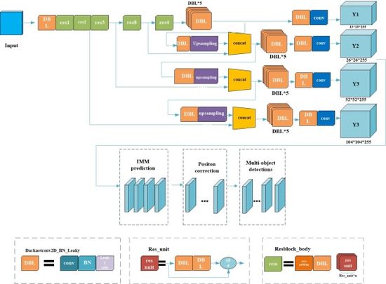
|
| Figure 1. Network architecture of our approach |
Figure 2 gives the flow chart of our model. It mainly contains two phases.
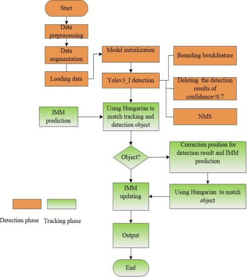
|
| Figure 2. General flow chart of our multi-object tracking model |
Detection phase:
Step 1: Split the original image into S*S cells or grids; each cell produces K bounding boxes according to the number of anchor boxes.
Step 2: Employ the convolutional neural network to get features and predict the , and the .
Step 3: Compare the maximum confidence of the bounding boxes with the threshold , if , the bounding box has the object. Else, the bounding boxes not contain the object.
Step 4: Select the class with the highest probability as the object category. Adopt NMS to operate a maximum part search for suppressing redundant boxes, output the results of object detection.
Tracking phase:
Step 1: Use IMM to predict tracks or Bbox for current frame. If objects are confirmed detection results and prediction tracks begin correlation and matching. Else, position correction algorithm is used for the unmatched tracks and detections.
Step 2: Update the tracked Bbox after the matching is completed.
Step 3: After updating, the current frame is predicted, the next frame is observed, and updated; then predicted again. The next frame is observed and updated, etc.
3.1. Improved YOLOv3 network
In traffic scenes, usually people, traffic lights, or cars in the input image has low resolution and is small objects, while the perceptual field of the convolutional layer at the end of the YOLOv3 backbone is very large. So it is a difficult task to detect the accurate objects with YOLOv3. In computer vision tasks, invariance and equivalent transformations are two important properties in image feature representation. Classification aims to learn high-level semantic information and therefore invariant feature representations are required. The goal of object localization is to distinguish between position and scale changes, so it requires equivalence transformations. Object detection consists of two subtasks, object identification, and localization. While learning invariance and equivalence transformations are the keys to detection. The YOLOv3 is composed of a series of convolutional and pooling layers. The deep-level features have stronger invariance, but their equivalence transformation is weak. Although this is beneficial for classification recognition, it suffers from low localization accuracy in object detection. On the contrary, the shallow layer features are not conducive to semantic learning, but it contains more edge and contour information, which helps in object localization. The combination of multi-scale features can increase the global and local feature information in the model to improve the accuracy of object detection and increase the accuracy of subsequent object tracking. Therefore, to boot the detection performance of the model for small objects in traffic scenes, this paper use feature fusion technique to enhances the prediction of YOLOv3 by further integrating deep and shallow features in the model, adding a one-dimensional scale to strengthen small object prediction, and adding a residual structure in the corresponding scale branch to effectively control the gradient propagation and prevent the gradient from disappearing, degrading the network, and not easily converging, which brings about unfavorable network training. The network is easy to converge. This makes the training of the deeper network less difficult. The structure of the improved Yolov3 network is shown in Figure 3. The detail fusion process can be described as follows:
|
|
(1) |
|
|
(2) |
Where indicates the r_th layer feature map of , belongs to stands for the action of convolution, BN, ReLu and tensor addition represents the p_th fused feature map. and shows the high-resolution feature map and low-resolution feature map, respectively. is the action of upsampling, is the action of full connection and represents the action of convolution. To describe the model later, the model is abbreviated as YOLOv3_I.
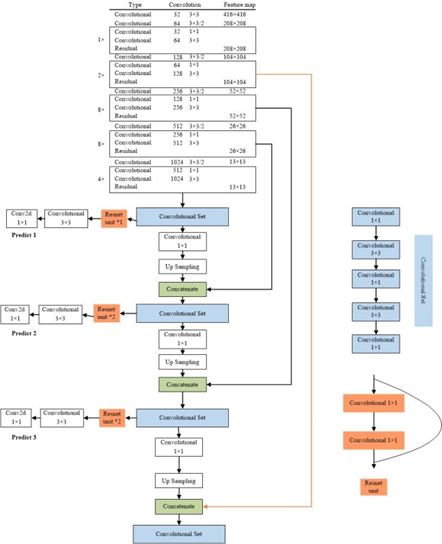
|
| Figure 3. The structure of YOLOv3_I network |
The model is similar to YOLOv3, with only convolution layers. The size of the output feature map is controlled by adjusting the convolution step, so there is no special restriction on the input image size. Also drawing on the pyramid feature map idea, the small size feature map is applied to detect large-size objects, while the large size feature map detects small size objects. Finally, according to analysis to dataset, a total of 4 feature maps are output, the first feature map is down-sampled 32 times, the second feature map 16 times, the third 8 times, and the fourth 4 times. Four detections, each corresponding to a different field of perception, 32 down-sampling has the largest field of perception, suitable for detecting large objects, 16 for objects of average size, 8 for the smallest field of perception, suitable for prediction small objects, and even smaller objects. Considering the fact that objects have different pixels, we use different scales of anchor boxes to match. The anchor size of each cell is shown in Table 1 according to object size of the MOT16. The whole network, which draws the essence of Resnet [27], Densenet [28], and FPN [29], incorporates the current industry effective techniques of object detection to detect the object.
| Feature map | 13*13 | 26*26 | 52*52 | 104*104 |
|---|---|---|---|---|
| Receptive field | Large | Medium | Less | Smallest |
| A prior box | (156*198) (156*198) (371*326) |
(30*61) (62*45) (59*119) |
(10*13) (16*30) (33*23) |
(10*11) (19*15) (25*21) |
3.2. Interactive multi-model algorithms
Due to the complexity of the actual motion of the objects in the traffic scene, it is difficult to describe the motion pattern of the objects using only one model. Therefore, the algorithm in this paper adopts the Interacting Multiple Model (IMM) [30] to estimate the motion patterns of multiple objects (Figure 4). Its main feature is the ability to approximate the state of dynamic systems with multiple patterns of behavior that can be switched from one behavior pattern to another. In particular, the IMM evaluator can be a self-tuning variable bandwidth filter, which allows it to naturally track maneuvering objects. IMM handles multi-object motion models in the Bayesian framework with a model set containing different motion sub-models, each corresponding to a filter. To solve the uncertainty of the object motion, each filter performs parallel operation computation and switches between models according to the updated weights. During object tracking, the fit of each sub-model of the system to the current object depends on the probability of the model. So, the interaction between models can be performed according to this principle, and finally the probabilistic output results of each sub-model are fused.
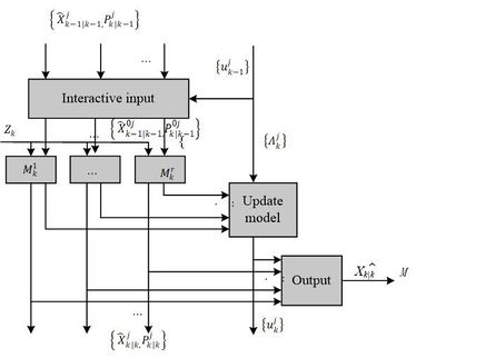
|
| Figure 4. Flow chart of IMM algorithm |
(1) Model initialization: denotes the j_th filter at the k_th frame, .
Model initialization state ; Covariance matrix :
|
(3) |
|
|
(4) |
Mixing probability = ; Normalization constants ; is the Markov transition probability of filter to .
(2) Model filtering estimation: in this paper, the standard IMM model is used, and the filtering phase has two main steps: prediction and correction. The prediction phase is responsible for calculating the a priori state estimates for each system in the current state. The correction phase is responsible for combining the actual measurements into each prior estimate to obtain the corresponding a posteriori state estimate. The motion and measurement models of the Kalman Filter are described as follows:
|
|
(5) |
|
|
(6) |
where is a priori state estimation. are state transition matrix, measurement matrix respectively. represents the measured value at the kth frame. and are the noise corresponding to the computational quantities obeying Gaussian distribution. Finally, the posterior state estimate is obtained
|
|
(7) |
is the residual of the motion model and the measurement model. filtering gain is defined as:
|
|
(8) |
where the a priori covariance matrix is:
|
|
(9) |
The posterior covariance matrix is updated as:
|
|
(10) |
(3) Model probability updating. Calculating model probabilities:
|
|
(11) |
|
|
(12) |
Likelihood function :
|
|
(13) |
The filter residual, ; , is the corresponding filtering residual matrix, and is Gaussian distribution. If the residuals are larger, it means that the model has a larger deviation from the object localization. Its weight decreases, and vice versa, the weight increases.
(4) Estimated fusion. Final state estimates and their covariances:
|
|
(14) |
|
|
(15) |
3.3 Position correction optimization algorithm
In traffic scenes, traffic objects such as cars and pedestrians are usually very dense. Especially in the event of traffic congestion, the objects are easily obscured and so on. When the object is obscured, the information of the object becomes incomplete and the object is easily lost. Therefore, in the paper, a position correction algorithm that fine-tunes the tracked object position is used in order to solve the lost-following phenomenon that occurs during the object tracking. The method corrects the object position based on the original predicted position, as shown in Figure 5. When the object is not found in the tracking area predicted by the IMM [31], the algorithm firstly considers that the object has been lost. Then, two points are selected from the location predicted by the IMM and the detection area of the detection algorithm. Eight-pixel points are added around it. Next, a fixed 125 threshold is set to compare the grayscale value of each point with the object empirical grayscale value. The last, we get the best point from the ten points and determine whether the point belongs to the object position.
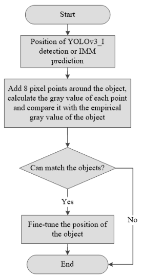
|
| Figure 5. Flowchart of position correction algorithm |
3.4 Implement detail
The training parameters of the network are set as follows: the parameter of leak ReLu ai is 10; the hyperparameters λnoobj, λobj, λcoord, λclass, λprior, of the loss function are 1,5,1,1 and 0.1; the Nprior is 11200. The adaptive moment estimation is adopted to update the weights of the network; the momentum is 0.9, the decay is 0.0005, the batch size is 32; the initial learning rate is 0.001, and the learning rate on the 300th epoch and the 400th epoch is set to 0.1 times of the original.
4. Experiment
4.1. Experiment preparation
The experiments are operated on the computer with Intel Core i7-7700 CPU, 3.5GHz, 8G DDR4, 2666MHz memory, and Nvidia GTX1080Ti, with Ubuntu Linux 18.04 and Python3. Deep learning framework is tensorflow.
The performance of the proposed detection model is proven on MOT16 and KITTI datasets. The KITTI dataset is a dataset for autonomous driving, with cars and pedestrians. The MOT16 dataset is proposed in 2016 to measure standards for multi-object tracking detection and tracking methods. The performance of the proposed multi-object tracking algorithm is evaluated on the public MOT16 dataset [32]. The MOT16 benchmark evaluates the tracking performance of challenging test sequences, including forward-looking scenes with moving cameras and top-down surveillance settings. The dataset was divided into a training set and validation set. Finally, it is compared with other multi-object tracking algorithms on the test set of MOT16. The evaluation metrics are:
MOTA: Multi-Object Tracking Accuracy:
|
|
(14) |
GT is the number of Groundtruth. FN stands for the missing number. The number of frames in which the object has no hypothetical position to match. FP is the number of object mismatches. The number of frames in which the given hypothetical position has no tracking object to match it. IDs is a mismatch. The number of times the tracking object has an ID switch in frame .
MOTP: Multi-object tracking accuracy:
|
|
(15) |
where represents the number of matches between objects and hypotheses in frame , and denotes the distance between objects and their paired hypothesis positions in frame .
4.2. The experiment results and analysis
The evaluation metric of the object detection commonly contains the mean Average Precision (mAP), the Average Precision (AP), F1 score, Recall rate, and so on. The mAP is considered the average of AP of all object categories. Thus, we use mAP and F1 scores as the authoritative metric to evaluate the performance of our model. Tables 2 and 3 introduce typical and related evaluation results on MOT16 and KITTI datasets.
| Model (Detector) | Recall | Precision |
|---|---|---|
| FrRCNN(VGG16) | 49.5% | 77.5% |
| FrRCNN(ZF) | 41.3% | 72.4% |
| YOLOv3 | 48.2% | 75.6% |
| YOLOv3_I | 50.1% | 77.4% |
| Model (Detector) | Recall | Precision |
|---|---|---|
| FrRCNN(VGG16) | 63.9% | 79.1% |
| FrRCNN(ZF) | 60.1% | 74.6% |
| YOLOv3 | 75.7% | 78.9% |
| YOLOv3_I | 79.8% | 81.1% |
Referring to the idea in SORT tracking algorithm, detection performance has a significant impact on tracking performance. A good detector can result in the best tracking accuracy [33]. Faster R-CNN is the popular and classical detection algorithm in the study. In this paper, we also hope to improve the tracking performance by improving the detector accuracy, as shown in Tables 2 and 3, YOLOv3_I outperforms Faster R-CNN in terms of object detection effect and has more advantages in detection speed and accuracy, which is more beneficial to have better behavior of multi-object tracking. In the process of pedestrian detection, the paper uses the parameters obtained from training in PASCAL VOC for initialization. The table compares two network architectures provided by FrRCNN, namely Zeiler and Fergus' architecture (FrRCNN(ZF)) [34] Simonyan and Zisserman's deeper architecture (FrRCNN(VGG16)) [35] and the paper's improved multi-scale fusion model based on YOLOv3, named YOLOv3_I which shows that the model used in this paper obtains better detection recall and accuracy. It can be facilitated the later object tracking. Figure 6 gives detection result of epoch vs loss on MOT16 and KITTI datasets. The proposed model compared with other models has good convergence speed. Figures 7 and 8 show the schematic diagrams of the detection output of the YOLOv3_I model, in which the corresponding confidence, classification, and localization are given for the detected objects. In the final tracking part of the experiments, only the objects with the detection probability confidence greater than 50% are passed to tracking model in the paper.
| ||
| Figure 6. YOLOv3_I detection epoch vs loss on MOT16 (left) and KITTI (right) |
| ||||||||
| Figure 7. YOLOv3_I detection results schematic diagram on MOT16 |
| ||||||||
| Figure 8. YOLOv3_I detection results schematic diagram on KITTI |
4.3. Analysis of experimental results of multi-object tracking model
The proposed method is compared with several existing object tracking methods on the MOT2016 to test the various performances of the algorithm, as shown in Table 4. All benchmark testing methods and our approach use the same publicly available test results for a fair comparison. The proposed method outperforms previous approaches in terms of MOTP, ML, and Frag. The offline tracking method can access all future detection results and reason on the data association step, and the results show that the MOTP of the proposed method is better than that of the offline method with about 3 percentage point higher performance. The technique using object correction can find the correct object after occlusion or drift. Therefore, our experiment results have higher MT and lower ML, but the IDS is higher. When the objects are occluded, the proposed method in the paper may incorrectly assign them to other detection objects. However, when the objects reappear, the methods proposed will re-match them with the correct detection results. Such a process can lead to a large number of switches. But the Frag metric is still high.
| Method | Mode | MOTA↑ | MOTP↑ | MT↑ | ML↓ | IDs↓ | Frag↓ |
|---|---|---|---|---|---|---|---|
| MCjoint [36] | Offline | 47.1 | 76.3 | 20.4 | 46.9 | 370 | 598 |
| SMOT [37] | Offline | 29.7 | 72.5 | 5.3 | 47.1 | 3108 | 4483 |
| NOMT [19] | Offline | 46.4 | 76.6 | 18.3 | 41.4 | 359 | 504 |
| LMP [38] | Offline | 48.8 | 79.0 | 18.2 | 40.1 | 481 | 595 |
| OVBT [39] | Online | 38.4 | 75.4 | 7.5% | 47.3% | 1321 | 2140 |
| EAMTT [40] | Online | 38.8 | 75.1 | 7.9% | 49.1% | 965 | 1657 |
| oICF [41] | Online | 43.2 | 74.3 | 11.3% | 48.5% | 381 | 1404 |
| SORT [33] | Online | 59.8 | 79.6 | 25.4 | 22.7 | 1101 | 1664 |
| Deep SORT [42] | Online | 61.4 | 79.1 | 32.8 | 18.2 | 781 | 1023 |
| Our | Online | 61.7 | 80.6 | 23.5 | 16.3 | 837 | 1705 |
The red boxes represent the person and give confidence for the corresponding objects. The red indicates the result of pedestrian tracking. The yellow numbers give the ID of the pedestrian tracking in Figure 9 (only the pedestrian ID is given because the objects are too dense). In this figure, cars or pedestrians move from far to near or near to far, showing the same class or the scale size of object change over time, which reflects the different scale changes of the object. Correspondingly, YOLOv3_I uses 4 scale features for fusion to obtain detection results in feature maps of different depths. Smaller objects can be detected in larger feature maps, while larger objects can be examined in relatively smaller feature maps, which can the detection objects at different scales.
| ||||||||||||||||||||||||||||||||||||||||||
| Figure 9. Results of our method on MOT16 (a,b,c,d,e,f,g) | ||||||||||||||||||||||||||||||||||||||||||
5. Conclusion
The traffic scenes are complex and changeable, which brings great difficult to implement the Intelligent Transportation System. In this paper, we propose a multi-object tracking method for traffic scenes. In multi-object detection, simple objects can be distinguished by using shallow features, while deeper features can identify more complex objects, so this paper uses multi-scale feature fusion technology to adapt to the changes of different scales of multi-object objects. A scale prediction is added to the original YOLOv3 network so that the accuracy of small object prediction can be increased, and the residual structure is also introduced to enhance the gradient propagation and avoid gradient disappearance or explosion. Next, the traffic scene is dense with objects and occlusion between objects tends to occur. When the tracked object is occluded, the information of the object becomes incomplete and thus the phenomenon of the lost happens. This paper develops a position correction algorithm to fine-tune the position of the tracked object. And when the object reappears, the occluded object can be matched with the correct detected object again. The IMM algorithm is also dedicated to the tracking stage to adapt to the complex object changes in the traffic scene and improve the tracking accuracy.
The proposed multi-object tracking method in this paper is mainly based on the mainstream idea of "detection + tracking", which achieves a certain tracking effect and has certain application value. However, for complex traffic scenarios, the method still has some shortcomings, so the follow-up work will be carried out. To improve the overall detection and tracking performance for multiple objects in a scene, the work can be considered to study the detection and tracking system in terms of the inter-influence relationship between objects, or the interconnectedness between traffic objects. Another research direction is to combine the object detection output results with the tracking model to further investigate detection-based end-to-end tracking algorithms.
Author Contributions: Conceptualization, C.R., H. Y., and W. L; Data curation, G.Z. and H. Y.; Formal analysis, C.R.; Funding acquisition, G.Z.; Investigation, G. Z., K. Z., H. Y. and S. Z.; Methodology, C.R., K. Z., S. Z. and W.L.; Project administration, G. Z.; Resources, G. Z., K. Z., H. Y.and S. Z.; Software, C. R. and W. L.; Validation, G. Z.; Visualization, K. Z. and S. Z.; Writing – original draft, C. R.; Writing – review & editing, K. Z. All authors have read and agreed to the published version of the manuscript.
Conflicts of Interest: The authors declare no conflict of interest.
Abbreviations
The following abbreviations are used in this manuscript:
| IMM: | Interacting Multiple Model |
| YOLOv3: | You Only Look Once Version3 |
| SVM: | Support Vector Machines |
| RPN: | Region Proposal Network |
| ITS: | Intelligent Transportation System |
| FP: | False Positive |
| FN: | False Negative |
| CNN: | Convolutional Neural Network |
| RoI: | Region of Interest |
References
[1] Xu Y., Zhou X., Chen S., Li F. Deep learning for multiple object tracking: a survey. IET Computer Vision, 13(4):355-368, 2019.
[2] Ciaparrone G., Sánchez F.L., Tabik S., Troiano L., Tagliaferri R., Herrera F. Deep learning in video multi-object tracking: A survey. Neurocomputing, 381:61-88, 2020.
[3] Li X., Wang K., Wang W., Li Y. A multiple object tracking method using Kalman filter. The 2010 IEEE international conference on information and automation, IEEE, pp. 1862-1866, 2010.
[4] Henriques J.F., Caseiro R., Martins P., Batista J. High-speed tracking with kernelized correlation filters. IEEE Transactions on Pattern Analysis and Machine Intelligence, 37(3):583-596, 2014.
[5] Li X., Hu W., Shen C., Zhang Z., Dick A., Hengel A. A survey of appearance models in visual object tracking. ACM transactions on Intelligent Systems and Technology (TIST), 4(4):1-48, 2013.
[6] LeCun Y., Bengio Y., Hinton G. Deep learning. Nature, 521:436-444, 2015.
[7] Yu F., Li W., Li Q., Liu Y., Shi X., Yan J. POI: multiple object tracking with high performance detection and appearance feature. European Conference on Computer Vision, Springer International Publishing, pp. 36-42, 2016.
[8] Zhang L., Gray H., Ye X., Collins L., Allinson N. Automatic individual pig detection and tracking in pig farms. Sensors, 19(5):1188, 2019.
[9] Zhao D., Fu H., Xiao L., Wu T., Dai B. Multi-object tracking with correlation filter for autonomous vehicle. Sensors, 18(7):2004, 2018.
[10] Wang Y., Wei X., Tang X., Shen H., Zhang H. Adaptive fusion CNN features for RGBT object tracking. IEEE Transactions on Intelligent Transportation Systems, 23(7):7831-7840, 2022.
[11] Xie Y., Shen J., Wu C. Affine geometrical region CNN for object tracking. IEEE Access, 8:68638-68648, 2020.
[12] Chintalacheruvu N., Muthukumar V. Video based vehicle detection and its application in intelligent transportation systems. Journal of Transportation Technologies, 2(04):305, 2012.
[13] Hinz G., Chen G., Aafaque M., Röhrbein F., Conradt J., Bing Z., Qu Z., Stechele W., Knoll A. Online multi-object tracking-by-clustering for intelligent transportation system with neuromorphic vision sensor. Joint German/Austrian Conference on Artificial Intelligence (Künstliche Intelligenz), Springer, pp. 142-154, 2017.
[14] Liang H., Song H., Li H., Dai Z. Vehicle counting system using deep learning and multi-object tracking methods. Transportation Research Record, 2674(4):114-128, 2020.
[15] Pino I. del, Vaquero V., Masini B.v Sola J., Moreno-Noguer F., Sanfeliu A., Andrade-Cetto J. Low resolution lidar-based multi-object tracking for driving applications. Iberian Robotics Conference, Springe, pp. 287-298, 2017.
[16] Liu Y., Li X., Bai T., Wang K., Wang F.Y. Multi-object tracking with hard-soft attention network and group-based cost minimization. Neurocomputing, 447:80-91, 2021.
[17] Abbas Q. V-ITS: Video-based intelligent transportation system for monitoring vehicle illegal activities. Int. J. Adv. Comput. Sci. Appl., 10(3):202-208, 2019.
[18] Dirir A., Adib M., Mahmoud A., Al-Gunaid M., El-Sayed H. An efficient multi-object tracking and counting framework using video streaming in urban vehicular environments. 2020 International Conference on Communications, Signal Processing, and their Applications (ICCSPA), IEEE, pp. 1-7, 2021.
[19] Nizar T.N., Anbarsanti N., Prihatmanto A.S. Multi-object tracking and detection system based on feature detection of the intelligent transportation system. 2014 IEEE 4th International Conference on System Engineering and Technology (ICSET), IEEE, pp. 1-6, 2014.
[20] Tian W., Lauer M., Chen L. Online multi-object tracking using joint domain information in traffic scenarios. IEEE Transactions on Intelligent Transportation Systems, 21(1):374-384, 2020.
[21] Rangesh A., Trivedi M.M. No blind spots: Full-surround multi-object tracking for autonomous vehicles using cameras and lidars. IEEE Transactions on Intelligent Vehicles, 4(4):588-599, 2019.
[22] Vasic M., Martinoli A. A collaborative sensor fusion algorithm for multi-object tracking using a Gaussian mixture probability hypothesis density filter. 2015 IEEE 18th International Conference on Intelligent Transportation Systems, IEEE, pp. 491-498, 2015.
[23] Emami P., Elefteriadou L., Ranka S. Long-range multi-object tracking at traffic intersections on low-power devices. IEEE Transactions on Intelligent Transportation Systems, 23(3):2482-2493, 2022.
[24] Gómez–Huélamo C., Bergasa L.M., Gutiérrez R., Arango J.F., Díaz A. SmartMOT: Exploiting the fusion of HDMaps and multi-object tracking for real-time scene understanding in intelligent vehicles applications. 2021 IEEE Intelligent Vehicles Symposium (IV), IEEE, Nagoya, Japan, pp. 710-715, 2021.
[25] Redmon J., Farhadi A. Yolov3: An incremental improvement. arXiv preprint arXiv:1804.02767, 2018.
[26] Faure F., Duriez C., Delingette H., Allard J., Gilles B., Marchesseau S., Talbot H., Courtecuisse H., Bousquet G., Peterlik I. Sofa: A multi-model framework for interactive physical simulation. Soft Tissue Biomechanical Modeling for Computer Assisted Surgery, Springer, vol. 11, 283-321, 2012.
[27] Wu Z., Shen C., Hengel A. Wider or deeper: Revisiting the resnet model for visual recognition. Pattern Recognition, 90:119-133, 2019.
[28] Iandola F., Moskewicz M., Karayev S., Girshick R., Darrell T., Keutzer K. Densenet: Implementing efficient convnet descriptor pyramids. arXiv preprint arXiv:1404.1869, 2014.
[29] Ghiasi G., Lin T.-Y., Le Q.V. Nas-fpn: Learning scalable feature pyramid architecture for object detection. Proceedings of the IEEE/CVF Conference on Computer Vision and Pattern Recognition, Long Beach, CA, USA, pp. 7029-7038, 2019.
[30] He R., Lee W.S., Ng H.T., Dahlmeier D. An interactive multi-task learning network for end-to-end aspect-based sentiment analysis. arXiv preprint arXiv:1906.06906, 2019.
[31] Welch G.F. Kalman filter. Computer vision: A reference guide, Springer, Cham, pp. 721-723, 2021.
[32] Dendorfer P., Rezatofighi H., Milan A., Shi J., Cremers D., Reid I., Roth S., Schindler K., Leal-Taixé L. Mot20: A benchmark for multi object tracking in crowded scenes. arXiv preprint arXiv:2003.09003, 2020.
[33] Fu H., Wu L., Jian M., Yang Y., Wang X., MF-SORT: Simple online and realtime tracking with motion features. International Conference on Image and Graphics, Springer, pp. 157-168, 2019.
[34] Zeiler M., Fergus R. Visualizing and understanding convolutional networks. arXiv 2013. 2019.
[35] Simonyan K., Zisserman A. Very deep convolutional networks for large-scale image recognition. arXiv preprint arXiv:1409.1556, 2018.
[36] Keuper M., Tang S., Zhongjie Y., Andres B., Brox T., Schiele B. A multi-cut formulation for joint segmentation and tracking of multiple objects. arXiv preprint arXiv:1607.06317, 2016.
[37] Choi W. Near-online multi-object tracking with aggregated local flow descriptor. 2015 IEEE Proceedings of the International Conference on Computer Vision, pp. 3029-3037, 2015.
[38] Tang S., Andriluka M., Andres B., Schiele B. Multiple people tracking by lifted multicut and person re-identification. 2017 IEEE Conference on Computer Vision and Pattern Recognition, pp. 3701-3710, 2017.
[39] Ban Y., Ba S., Alameda-Pineda X., Horaud R. Tracking multiple persons based on a variational Bayesian model. European Conference on Computer Vision – ECCV 2016 Workshops, Lecture Notes in Computer Science, Springer, Cham, pp. 52-67, 2016.
[40] Sanchez-Matilla R., Poiesi F., Cavallaro A. Online multi-object tracking with strong and weak detections. European Conference on Computer Vision – ECCV 2016 Workshops, Lecture Notes in Computer Science, Springer, Cham, pp. 84-99, 2016.
[41] Kieritz H., Becker S., Hübner W., Arens M. Online multi-person tracking using integral channel features. 2016 13th IEEE International Conference on Advanced Video and Signal Based Surveillance (AVSS), IEEE, Colorado Springs, CO, USA, pp. 122-130, 2016.
[42] Wojke N., Bewley A., Paulus D. Simple online and realtime tracking with a deep association metric. 2017 IEEE International Conference on Image Processing (ICIP), IEEE, Beijing, China, pp. 3645-3649, 2017.Document information
Published on 29/11/23
Accepted on 04/11/23
Submitted on 27/07/23
Volume 39, Issue 4, 2023
DOI: 10.23967/j.rimni.2023.11.001
Licence: CC BY-NC-SA license
Share this document
claim authorship
Are you one of the authors of this document?
