(Tag: Visual edit) |
Ferminotero (talk | contribs) m (Ferminotero moved page Review 602617684658 to Rubio et al 2023a) |
||
| (4 intermediate revisions by one other user not shown) | |||
| Line 14: | Line 14: | ||
|} | |} | ||
--> | --> | ||
| − | |||
| − | |||
| − | |||
| − | |||
| − | |||
| − | |||
| − | |||
| − | |||
| − | |||
| − | |||
| − | |||
| − | |||
| − | |||
| − | |||
| − | |||
| − | |||
| − | |||
| − | |||
| − | |||
| − | |||
| − | |||
==1 Introduction== | ==1 Introduction== | ||
| Line 42: | Line 21: | ||
Among the several options available, we will make use of the multiscale method for periodic structures using domain decomposition and ECM-hyperreduction proposed by the third author in Ref. <span id='citeF-1'></span>[[#cite-1|[1]]]. The reason for favouring this approach is its outcome is the stiffness matrix of a beam element that can be directly assembled in the same fashion as standard FE elements. Since this stiffness matrix is obtained from a set of numerical experiments it naturally captures the orthotropy present in composite materials, but its integration in FE codes poses a challenging framework which we tried to address. The difficulty resides in two distinctive aspects: the first is the number of DoF resulting from <span id='citeF-1'></span>[[#cite-1|[1]]] may differ from the classical beam theories; and the second is that the element size is fixed. | Among the several options available, we will make use of the multiscale method for periodic structures using domain decomposition and ECM-hyperreduction proposed by the third author in Ref. <span id='citeF-1'></span>[[#cite-1|[1]]]. The reason for favouring this approach is its outcome is the stiffness matrix of a beam element that can be directly assembled in the same fashion as standard FE elements. Since this stiffness matrix is obtained from a set of numerical experiments it naturally captures the orthotropy present in composite materials, but its integration in FE codes poses a challenging framework which we tried to address. The difficulty resides in two distinctive aspects: the first is the number of DoF resulting from <span id='citeF-1'></span>[[#cite-1|[1]]] may differ from the classical beam theories; and the second is that the element size is fixed. | ||
| − | The integration strategy | + | The integration strategy consists of two different stages. The first is the so-called condensation, from which the <math display="inline">n \times n</math> stiffness matrix is condensed into a matrix of size <math display="inline">12 \times 12</math> for a given beam length. Condensation will be used to create a database of stiffness matrices over which a regression is then performed. |
In the present work, the methodology will be briefly presented, but the main focus is on its application in a real case scenario under the scope of the EU funded project FIBRE4YARDS. | In the present work, the methodology will be briefly presented, but the main focus is on its application in a real case scenario under the scope of the EU funded project FIBRE4YARDS. | ||
| Line 71: | Line 50: | ||
|} | |} | ||
| − | where <math display="inline">u_D</math> are the prescribed displacements, c characterizes the linear relation between each boundary condition and the Lagrange multipliers <math display="inline">\lambda </math> associated. Periodic boundary conditions over the deformational modes are prescribed as they are in agreement with the classical theories for the case of isotropic materials. Following this strategy, we can account for the deformation inside the domain with the maximum resolution the method provides (conversely, should we truncate the stiffness matrix, we would get a stiffer response than the actual | + | where <math display="inline">u_D</math> are the prescribed displacements, c characterizes the linear relation between each boundary condition and the Lagrange multipliers <math display="inline">\lambda </math> associated. Periodic boundary conditions over the deformational modes are prescribed as they are in agreement with the classical theories for the case of isotropic materials. Following this strategy, we can account for the deformation inside the domain with the maximum resolution the method provides (conversely, should we truncate the stiffness matrix, we would get a stiffer response than the actual; for this reason, we discarded the option of using truncation). |
===2.3 Interpolation=== | ===2.3 Interpolation=== | ||
| Line 169: | Line 148: | ||
|} | |} | ||
| − | Before moving onto the condensation and regression stages, we must ensure the ROM can reproduce FE solutions. To do so, we have | + | Before moving onto the condensation and regression stages, we must ensure the ROM can reproduce FE solutions. To do so, we have solved a full-scale FE simulation and compared the solution with the ROM. The simulation is a 2m long clamped beam under a uniform load of 1 MPa in the other end, as shown in Figure [[#img-3|3]]. The surface dimensions are 0.0256 <math display="inline">\times </math> 0.01m |
<div id='img-3a'></div> | <div id='img-3a'></div> | ||
| Line 185: | Line 164: | ||
|} | |} | ||
| − | Figure [[#img-4|4]] presents the solution for FE and ROM. It can be seen that the | + | Figure [[#img-4|4]] presents the solution for FE and ROM. It can be seen that the results are very similar, although the ROM is a bit more flexible than the FE. This discrepancy is expected as the ROM cannot capture boundary effects, but as we move away from the edge of the beam, both solutions converge. On top of this, the training was made prescribing periodic boundary conditions on the slice, hence softer elements in ROM are expected. |
<div id='img-4a'></div> | <div id='img-4a'></div> | ||
| Line 203: | Line 182: | ||
Once checked the ROM can reproduce FE simulations, we can proceed to the condensation stage. The results of the condensation must be analysed carefully. Cross terms appear due to two reasons: material orthotropy and geometrical coupling. The latter is due to the fact that the shear centre and centroid, in profiles with only one axis of symmetry, do not coincide <span id="fnc-1"></span>[[#fn-1|<sup>1</sup>]] and thus coupling between torsion and bending and shear in the non-symmetric plane appears; the former is caused by the material behavior itself. | Once checked the ROM can reproduce FE simulations, we can proceed to the condensation stage. The results of the condensation must be analysed carefully. Cross terms appear due to two reasons: material orthotropy and geometrical coupling. The latter is due to the fact that the shear centre and centroid, in profiles with only one axis of symmetry, do not coincide <span id="fnc-1"></span>[[#fn-1|<sup>1</sup>]] and thus coupling between torsion and bending and shear in the non-symmetric plane appears; the former is caused by the material behavior itself. | ||
| − | To discern the geometrical coupling, the same geometry with an isotropic material has been trained and | + | To discern the geometrical coupling, the same geometry with an isotropic material has been trained and computed. Figure [[#img-5|5]] represents the evolution of the stiffness matrix values (obtained with the condensation procedure) as a function of the beam length. The non-zero values of terms 2,3 and 1,5 prove the geometrical coupling is non-negligible. |
Since geometrical coupling is a property of the cross-sectional shape, we can make sure any other coupling is caused by the orthotropy of the material, as it is the case of the terms <math display="inline">k_{23}</math> and <math display="inline">k_{15}</math> (see Figure [[#img-6|6]]). This material orthotropy is precisely the one that cannot be captured by classical beam theories but naturally appear following <span id='citeF-1'></span>[[#cite-1|[1]]] and the strategy presented in section [[#2 Methodology|2]]. | Since geometrical coupling is a property of the cross-sectional shape, we can make sure any other coupling is caused by the orthotropy of the material, as it is the case of the terms <math display="inline">k_{23}</math> and <math display="inline">k_{15}</math> (see Figure [[#img-6|6]]). This material orthotropy is precisely the one that cannot be captured by classical beam theories but naturally appear following <span id='citeF-1'></span>[[#cite-1|[1]]] and the strategy presented in section [[#2 Methodology|2]]. | ||
| Line 228: | Line 207: | ||
===3.1 Validation=== | ===3.1 Validation=== | ||
| − | Lastly, we must check whether to process of condensation plus regression gives similar solutions than the full ROM. To so do we have | + | Lastly, we must check whether to process of condensation plus regression gives similar solutions than the full ROM. To so do we have computed the same case with the full ROM and the condensed model with 3 different element sizes. Figure [[#img-7|7]] shows the displacements and rotations along the beam for the loading case studied (see Figure [[#img-3|3]]). It can be observed that, as the element size gets closer to 10cm (a point in the database), the 6 DoF solution is able to reproduce the full ROM results. In addition, no instabilities appear in any of the 3 element sizes so we can consider the methodology presented in this work is validated for orthotropic materials. |
<div id='img-7'></div> | <div id='img-7'></div> | ||
Latest revision as of 09:33, 10 October 2023
1 Introduction
Numerical methods for Partial Differential Equations (PDE) result in high dimensional systems of equations. One prominent example is the finite element method, which has seen its most valuable attributes, the diversity and resolution it provides, become prohibitive in terms of computer resources and time. Reduced order models (ROM) try to alleviate the computational cost seeking solutions in a lower dimensional space. One could envisage classical analytical derivations like Euler-Bernoulli or Timoshenko's beam theories as the first ROM, since, following certain assumptions, they cast the kinematics of one-dimensional specimens only in terms of 6 degrees of freedom. Such analytical derivations, however, are restricted to (relatively) ideal configurations and hence not extensible to more complex engineering problems like composite materials which are widely used in a great number of applications. In addition, today's technologies namely additive manufacturing or pultrusion make these composite materials much more attractive due to its high quality end product which, in turn, further justifies the development of accurate and fast ROM beyond analytical solutions.
Among the several options available, we will make use of the multiscale method for periodic structures using domain decomposition and ECM-hyperreduction proposed by the third author in Ref. [1]. The reason for favouring this approach is its outcome is the stiffness matrix of a beam element that can be directly assembled in the same fashion as standard FE elements. Since this stiffness matrix is obtained from a set of numerical experiments it naturally captures the orthotropy present in composite materials, but its integration in FE codes poses a challenging framework which we tried to address. The difficulty resides in two distinctive aspects: the first is the number of DoF resulting from [1] may differ from the classical beam theories; and the second is that the element size is fixed.
The integration strategy consists of two different stages. The first is the so-called condensation, from which the stiffness matrix is condensed into a matrix of size for a given beam length. Condensation will be used to create a database of stiffness matrices over which a regression is then performed.
In the present work, the methodology will be briefly presented, but the main focus is on its application in a real case scenario under the scope of the EU funded project FIBRE4YARDS.
2 Methodology
2.1 A multiscale method for periodic structures using domain decomposition and ECM-hyperreduction
In this section we will briefly describe the approach proposed in Ref. [1] as it is the starting point of our methodology. In the multiscale method for periodic structures using domain decomposition and ECM-hyperreduction the original PDE is solved without any simplification (other than those of FE) but the solutions are sought in a lower dimensional space. This lower dimensional space is extracted from a set of high fidelity (FE) simulations, in a so-called offline stage. In other words, several FE simulations are run and their results processed to find a reduced approximation of the data. This reduced approximation is then used to solve the original PDE (note that the boundary conditions need not to be the same as for the training), in a so-called online stage.
Two features form the core of this method, one is the domain decomposition based on Local Lagrange Multipliers (LLM) [2] and the second is dimensionality reduction by means of the Singular Value Decomposition (SVD). LLM introduces fictitious interfaces between adjacent subdomains that play the role of coarse-scale mesh, the displacements of which constitute the primal unknown of the ROM. On its own, though, domain decomposition does not lead to a lower dimensional parameterization of the system, hence the need of the SVD (SVD gives a reduced basis that best approximates the data from the offline stage). The combination of both features result in a model with the coarse scale displacement parameterized by a reduced set of basis vectors. For a complete description of the method we refer to [1], [3].
2.2 Condensation
As already mentioned, the reduced basis resulting from the method described in the foregoing may involve more than 6 DoF per node, hence the motivation of the integration strategy described here. As mentioned, the integration strategy consist of two phases: a condensation process followed by a regression procedure.
The objective of the condensation is to obtain a matrix of size 12×12 (for a given element size) from a n × n matrix. To do so we discretize a beam of a certain length in N elements using the n × n matrix; we then apply perturbations at every end and retain the reactions corresponding to rigid body motion. To do so, we set the external forces to 0 and solve the equilibrium equations with the prescribed boundary conditions:
|
|
(1) |
where are the prescribed displacements, c characterizes the linear relation between each boundary condition and the Lagrange multipliers associated. Periodic boundary conditions over the deformational modes are prescribed as they are in agreement with the classical theories for the case of isotropic materials. Following this strategy, we can account for the deformation inside the domain with the maximum resolution the method provides (conversely, should we truncate the stiffness matrix, we would get a stiffer response than the actual; for this reason, we discarded the option of using truncation).
2.3 Interpolation
Condensation is used to create a database of stiffness matrix as a function of the specimen length over which a regression is performed. Two different strategies have been investigated, a global interpolation within the logarithmic space and a linear interpolation with local support (in the same fashion as 1D FE [4]). Both strategies accurately fit the data, but the global interpolation may lead to instabilities when assembling several elements obtained by the global function. Hence, we recommend the use of functions with local support to get stable elements:
|
|
(2) |
where and are the stiffness matrices at the end points of the segment and l the desired element size.
3 Case study
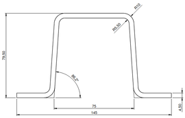
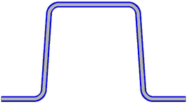
This section is devoted to the numerical analysis of the real pultruded profile to be build under the scope of FIBRE4YARDS. The profile (shown in Figure 1) is a laminate composite material: the central layer is made of unidirectional glass fibre reinforced material, while the top and bottom layers are themselves laminates as well.
|
|
| (a) | (b) |
| Figure 1: (a) Cross-sectional dimensions (b) Gray: unidirectional material. Blue:laminate | |
The mechanical properties listed below are computed by the serial-parallel mixing theory [5]:
| [Pa] | [Pa] | [Pa] | [Pa] | [Pa] | [Pa] | ||||
| Unidirectional | 0.0466 | 0.0466 | 0.0466 | ||||||
| Laminate | 0.299 | 0.0471 | 0.0471 |
Figure 2 shows the deformational, self-equilibrated and interface modes resulting from [1]. It can be observed that although there are 8 self-equilibrated modes, the interface modes reduce to 7 (3 translation, 3 rotations and the out-of-plane warping mode). This fact is due to the periodicity imposed in the ROM, i.e. all interfaces must have the same modes (so that they fit together) and hence only the common ones are retained.

|

|
| (a) | (b) |

| |
| (c) | |
| Figure 2: (a) Subdomain deformational modes (b) Self-equilibrated modes (c) Interface modes | |
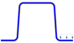
Before moving onto the condensation and regression stages, we must ensure the ROM can reproduce FE solutions. To do so, we have solved a full-scale FE simulation and compared the solution with the ROM. The simulation is a 2m long clamped beam under a uniform load of 1 MPa in the other end, as shown in Figure 3. The surface dimensions are 0.0256 0.01m
| |
| (a) | (b) |
| Figure 3: (a) 3D representation of the beam, in red the surface onto which the load is prescribed (b) Cross sectional representation of the load | |
Figure 4 presents the solution for FE and ROM. It can be seen that the results are very similar, although the ROM is a bit more flexible than the FE. This discrepancy is expected as the ROM cannot capture boundary effects, but as we move away from the edge of the beam, both solutions converge. On top of this, the training was made prescribing periodic boundary conditions on the slice, hence softer elements in ROM are expected.

|

|
| (a) | (b) |
| Figure 4: (a) Z displacement FE solution (b) Z displacement ROM solution | |
Once checked the ROM can reproduce FE simulations, we can proceed to the condensation stage. The results of the condensation must be analysed carefully. Cross terms appear due to two reasons: material orthotropy and geometrical coupling. The latter is due to the fact that the shear centre and centroid, in profiles with only one axis of symmetry, do not coincide 1 and thus coupling between torsion and bending and shear in the non-symmetric plane appears; the former is caused by the material behavior itself.
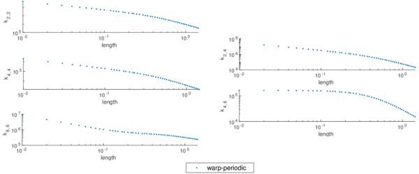
To discern the geometrical coupling, the same geometry with an isotropic material has been trained and computed. Figure 5 represents the evolution of the stiffness matrix values (obtained with the condensation procedure) as a function of the beam length. The non-zero values of terms 2,3 and 1,5 prove the geometrical coupling is non-negligible.
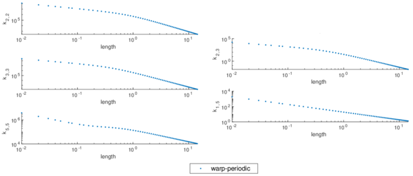
Since geometrical coupling is a property of the cross-sectional shape, we can make sure any other coupling is caused by the orthotropy of the material, as it is the case of the terms and (see Figure 6). This material orthotropy is precisely the one that cannot be captured by classical beam theories but naturally appear following [1] and the strategy presented in section 2.
|
| Figure 5: Results of the condensation for the omega profile with isotropic material. Units in IS |
|
| Figure 6: Results of the condensation for the omega profile with the properties shown in table 1. Units in IS |
(1) The ROM reference point is the geometrical centroid not the shear centre. When these two point do not coincide bending is coupled with torsion in the non-symmetry plane
3.1 Validation
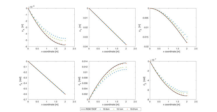
Lastly, we must check whether to process of condensation plus regression gives similar solutions than the full ROM. To so do we have computed the same case with the full ROM and the condensed model with 3 different element sizes. Figure 7 shows the displacements and rotations along the beam for the loading case studied (see Figure 3). It can be observed that, as the element size gets closer to 10cm (a point in the database), the 6 DoF solution is able to reproduce the full ROM results. In addition, no instabilities appear in any of the 3 element sizes so we can consider the methodology presented in this work is validated for orthotropic materials.
| Figure 7: Comparison of the solution with 7 DoF and 6DoF for the Omega profile |
4 Conclusions
This work presents the validation of the integration strategy proposed in Ref. [1] into standard FE code for the case of orthotropic beams. Concerning the training stage, periodic boundary conditions lead to softer elements compared to FE (for a lenght of 2m), however, this difference is expected to vanish for more slender beams. The results of the condensation plus regression show how the 6 DoF solution approach the one with 7 DoF for arbitrary element sizes. Furthermore, the elements resulting from the process are stable (for interpolations with local support) and hence, we can state that the methodology presented will provide reliable solutions when integrated in standard FE codes.
Acknowledgement
This research was supported by the European Commission under grant agreement No 101006860. We thank our colleagues from FIBRE4YARDS who provided insight and expertise that greatly assisted the research.
BIBLIOGRAPHY
[1] J.A. Hernández. (2020) "A multiscale method for periodic structures using domain decomposition and ECM-hyperreduction", Volume 368. Computer Methods in Applied Mechanics and Engineering 113-192
[2] K.C. Park and C.A. Felippa. (2000) "A variational principle for the formulation of partitioned structural systems", Volume 47. Numerical Methods in Engineering 395-418
[3] A. Giuliodori and J.A. Hernández and E. Soudah. (2023) "Multiscale modeling of prismatic heterogeneous structures based on a localized hyperreduced-order method", Volume 407. Computer Methods in Applied Mechanics and Engineering 115913
[4] T. Hughes (2012) "The Finite Element Method: Linear Static and Dynamic Finite Element Analysis". Dover Publications
[5] F.Rastellini and S. Oller and O. Salomón and E. Oñate. (2008) "Composite materials non-linear modelling for long fibre-reinforced laminates: Continuum basis, computational aspects and validations", Volume 86. Computers & Structures 9 879-896
Document information
Published on 29/04/25
Accepted on 09/10/23
Submitted on 18/05/23
Volume 08 - COMUNICACIONES MATCOMP21 (2022) Y MATCOMP23 (2023), Issue Núm. 8 - Fabricación y Aplicaciones Industriales - Materiales y Estructuras - Modelos Numéricos, 2025
DOI: https://doi.org/10.23967/r.matcomp.2025.08.12
Licence: Other
