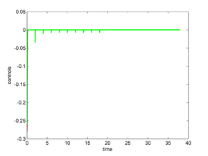
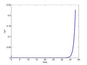
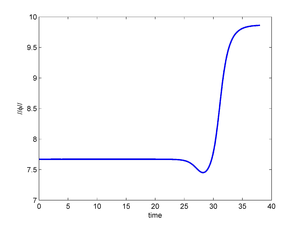
| (19 intermediate revisions by 2 users not shown) | |||
| Line 10: | Line 10: | ||
| − | Héctor Juárez Valencia | + | Héctor Juárez Valencia |
Universidad Autónoma Metropolitana, Iztapalapa | Universidad Autónoma Metropolitana, Iztapalapa | ||
| Line 23: | Line 23: | ||
==Abstract== | ==Abstract== | ||
| − | '''In this paper we consider a system of three nonlinear ordinary | + | '''In this paper we consider a system of three nonlinear ordinary differential equations that model a three Josephson Junctions Array (JJA). Our goal is to stabilize the system around an unstable equilibrium employing an optimal control approach. We first define the cost functional and calculate its differential by using perturbation analysis and variational calculus. For the computational solution of the optimality system we consider a conjugate gradient algorithm for quadratic functionals in Hilbert spaces, combined with a finite difference discretization of the involucrated differential equations.''' |
| − | ''Key word:'' Josephson Junction, Cryogenic Memory, Conjugate Gradient | + | ''Key word:'' Josephson Junction, Cryogenic Memory, Conjugate Gradient Algorithms, Stabilization, Optimal Control. |
MSC[2010] 65K10, 49M25. | MSC[2010] 65K10, 49M25. | ||
| − | == | + | ==1 Introduction== |
In this article we discuss the numerical simulation of a control approach to stabilize a Josephson Junction Array (JJA) around an unstable steady state. Our methodology relies significantly on a conjugate gradient algorithm operating in a well-chosen control space. It has been shown recently that such an array can carry out the functions of a memory cell operations (<span id='citeF-1'></span><span id='citeF-2'></span><span id='citeF-3'></span><span id='citeF-4'></span><span id='citeF-5'></span>[[#cite-1|[1,2,3,4,5]]]), consequently this array is frequently referred as a Josephson junction array memory (JJAM). | In this article we discuss the numerical simulation of a control approach to stabilize a Josephson Junction Array (JJA) around an unstable steady state. Our methodology relies significantly on a conjugate gradient algorithm operating in a well-chosen control space. It has been shown recently that such an array can carry out the functions of a memory cell operations (<span id='citeF-1'></span><span id='citeF-2'></span><span id='citeF-3'></span><span id='citeF-4'></span><span id='citeF-5'></span>[[#cite-1|[1,2,3,4,5]]]), consequently this array is frequently referred as a Josephson junction array memory (JJAM). | ||
| Line 90: | Line 90: | ||
|} | |} | ||
| − | The ''Read/Write'' operations can be performed by applying appropriate Gaussian pulses (<span id='citeF-1'></span>[[#cite-1|[1]]], <span id='citeF-4'></span>[[#cite-4|[4]]], <span id='citeF-5'></span>[[#cite-5|[5]]] ) in order to drive the system from an equilibrium configuration to another one. In <span id='citeF-9'></span>[[#cite-9|[9]]], we went beyond Gaussian pulses and investigated an optimal controllability approach in <math display="inline">L^2</math> to perform these transitions between equilibrium | + | The ''Read/Write'' operations can be performed by applying appropriate Gaussian pulses (<span id='citeF-1'></span>[[#cite-1|[1]]], <span id='citeF-4'></span>[[#cite-4|[4]]], <span id='citeF-5'></span>[[#cite-5|[5]]] ) in order to drive the system from an equilibrium configuration to another one. In <span id='citeF-9'></span>[[#cite-9|[9]]], we went beyond Gaussian pulses and investigated an optimal controllability approach in <math display="inline">L^2</math> to perform these transitions between equilibrium configurations. These approach is closely related to the methodology discussed in <span id='citeF-10'></span>[[#cite-10|[10]]] for systems modelled by partial differential equations. |
For the driving currents and coupling parameters provided in ([[#eq-3|3]]) and ([[#eq-4|4]]), the ordinary differential equation systems ([[#eq-5|5]]) (and ([[#eq-2|2]]) with <math display="inline">\dfrac{d\boldsymbol{\phi }}{dt}(0)=\boldsymbol{0 }</math>) have several steady state solutions, consisting of phase triplets. In many cases, the steady state phases are near the values <math display="inline">2\pi n_{k}</math>, for certain integers <math display="inline">n_{k}</math>, and, according to Braiman, et. al., (<span id='citeF-1'></span>[[#cite-1|[1]]]), equilibrium junction phases can be defined by their offsets <math display="inline">\sigma _k</math> from the negative cosine function's minima, as shown in the following equation | For the driving currents and coupling parameters provided in ([[#eq-3|3]]) and ([[#eq-4|4]]), the ordinary differential equation systems ([[#eq-5|5]]) (and ([[#eq-2|2]]) with <math display="inline">\dfrac{d\boldsymbol{\phi }}{dt}(0)=\boldsymbol{0 }</math>) have several steady state solutions, consisting of phase triplets. In many cases, the steady state phases are near the values <math display="inline">2\pi n_{k}</math>, for certain integers <math display="inline">n_{k}</math>, and, according to Braiman, et. al., (<span id='citeF-1'></span>[[#cite-1|[1]]]), equilibrium junction phases can be defined by their offsets <math display="inline">\sigma _k</math> from the negative cosine function's minima, as shown in the following equation | ||
| Line 132: | Line 132: | ||
|- style="border-top: 2px solid;" | |- style="border-top: 2px solid;" | ||
| colspan='1' style="text-align: left;border-left: 2px solid;border-right: 2px solid;border-left: 2px solid;border-right: 2px solid;" | <math>1</math> | | colspan='1' style="text-align: left;border-left: 2px solid;border-right: 2px solid;border-left: 2px solid;border-right: 2px solid;" | <math>1</math> | ||
| − | | colspan='1' style="text-align: left;border-left: 2px solid;border-right: 2px solid;border-left: 2px solid;border-right: 2px solid;" | <math> | + | | colspan='1' style="text-align: left;border-left: 2px solid;border-right: 2px solid;border-left: 2px solid;border-right: 2px solid;" | <math>0</math> |
| colspan='1' style="text-align: left;border-left: 2px solid;border-right: 2px solid;border-left: 2px solid;border-right: 2px solid;" | <math>0 (s)</math> | | colspan='1' style="text-align: left;border-left: 2px solid;border-right: 2px solid;border-left: 2px solid;border-right: 2px solid;" | <math>0 (s)</math> | ||
| − | | colspan='1' style="text-align: left;border-left: 2px solid;border-right: 2px solid;border-left: 2px solid;border-right: 2px solid;" | | + | | colspan='1' style="text-align: left;border-left: 2px solid;border-right: 2px solid;border-left: 2px solid;border-right: 2px solid;" | |
| − | | colspan='1' style="text-align: left;border-left: 2px solid;border-right: 2px solid;border-left: 2px solid;border-right: 2px solid;" | | + | | colspan='1' style="text-align: left;border-left: 2px solid;border-right: 2px solid;border-left: 2px solid;border-right: 2px solid;" | |
| − | | colspan='1' style="text-align: left;border-left: 2px solid;border-right: 2px solid;border-left: 2px solid;border-right: 2px solid;" | | + | | colspan='1' style="text-align: left;border-left: 2px solid;border-right: 2px solid;border-left: 2px solid;border-right: 2px solid;" | no |
| − | | style="border-left: 2px solid;border-right: 2px solid;" | | + | | style="border-left: 2px solid;border-right: 2px solid;" | stable |
| − | | style="border-left: 2px solid;border-right: 2px solid;" | | + | | style="border-left: 2px solid;border-right: 2px solid;" | equil |
| − | | style="border-left: 2px solid;border-right: 2px solid;" | | + | | style="border-left: 2px solid;border-right: 2px solid;" | |
|- style="border-top: 2px solid;" | |- style="border-top: 2px solid;" | ||
| colspan='1' style="text-align: left;border-left: 2px solid;border-right: 2px solid;border-left: 2px solid;border-right: 2px solid;" | <math>1</math> | | colspan='1' style="text-align: left;border-left: 2px solid;border-right: 2px solid;border-left: 2px solid;border-right: 2px solid;" | <math>1</math> | ||
| Line 180: | Line 180: | ||
| style="border-left: 2px solid;border-right: 2px solid;" | <math>12.2884</math> | | style="border-left: 2px solid;border-right: 2px solid;" | <math>12.2884</math> | ||
| style="border-left: 2px solid;border-right: 2px solid;" | <math>0.2092</math> | | style="border-left: 2px solid;border-right: 2px solid;" | <math>0.2092</math> | ||
| + | |- style="border-top: 2px solid;" | ||
| + | | colspan='1' style="text-align: left;border-left: 2px solid;border-right: 2px solid;border-left: 2px solid;border-right: 2px solid;" | <math>1</math> | ||
| + | | colspan='1' style="text-align: left;border-left: 2px solid;border-right: 2px solid;border-left: 2px solid;border-right: 2px solid;" | <math>0</math> | ||
| + | | colspan='1' style="text-align: left;border-left: 2px solid;border-right: 2px solid;border-left: 2px solid;border-right: 2px solid;" | <math>0 (u)</math> | ||
| + | | colspan='1' style="text-align: left;border-left: 2px solid;border-right: 2px solid;border-left: 2px solid;border-right: 2px solid;" | <math>0.0908</math> | ||
| + | | colspan='1' style="text-align: left;border-left: 2px solid;border-right: 2px solid;border-left: 2px solid;border-right: 2px solid;" | <math>0.3591</math> | ||
| + | | colspan='1' style="text-align: left;border-left: 2px solid;border-right: 2px solid;border-left: 2px solid;border-right: 2px solid;" | <math>-0.4140</math> | ||
| + | | style="border-left: 2px solid;border-right: 2px solid;" | <math>6.8539</math> | ||
| + | | style="border-left: 2px solid;border-right: 2px solid;" | <math>2.2566</math> | ||
| + | | style="border-left: 2px solid;border-right: 2px solid;" | <math>-2.6015</math> | ||
| + | |- style="border-top: 2px solid;" | ||
| + | | colspan='1' style="text-align: left;border-left: 2px solid;border-right: 2px solid;border-left: 2px solid;border-right: 2px solid;" | <math>2</math> | ||
| + | | colspan='1' style="text-align: left;border-left: 2px solid;border-right: 2px solid;border-left: 2px solid;border-right: 2px solid;" | <math>1</math> | ||
| + | | colspan='1' style="text-align: left;border-left: 2px solid;border-right: 2px solid;border-left: 2px solid;border-right: 2px solid;" | <math>0 (u)</math> | ||
| + | | colspan='1' style="text-align: left;border-left: 2px solid;border-right: 2px solid;border-left: 2px solid;border-right: 2px solid;" | <math>0.1011</math> | ||
| + | | colspan='1' style="text-align: left;border-left: 2px solid;border-right: 2px solid;border-left: 2px solid;border-right: 2px solid;" | <math>0.4539</math> | ||
| + | | colspan='1' style="text-align: left;border-left: 2px solid;border-right: 2px solid;border-left: 2px solid;border-right: 2px solid;" | <math>-0.0125</math> | ||
| + | | style="border-left: 2px solid;border-right: 2px solid;" | <math>13.2016</math> | ||
| + | | style="border-left: 2px solid;border-right: 2px solid;" | <math>9.1355</math> | ||
| + | | style="border-left: 2px solid;border-right: 2px solid;" | <math>-0.0786</math> | ||
| + | |- style="border-top: 2px solid;" | ||
| + | | colspan='1' style="text-align: left;border-left: 2px solid;border-right: 2px solid;border-left: 2px solid;border-right: 2px solid;" | <math>2</math> | ||
| + | | colspan='1' style="text-align: left;border-left: 2px solid;border-right: 2px solid;border-left: 2px solid;border-right: 2px solid;" | <math>2</math> | ||
| + | | colspan='1' style="text-align: left;border-left: 2px solid;border-right: 2px solid;border-left: 2px solid;border-right: 2px solid;" | <math>0 (u)</math> | ||
| + | | colspan='1' style="text-align: left;border-left: 2px solid;border-right: 2px solid;border-left: 2px solid;border-right: 2px solid;" | <math>0.1576</math> | ||
| + | | colspan='1' style="text-align: left;border-left: 2px solid;border-right: 2px solid;border-left: 2px solid;border-right: 2px solid;" | <math>-0.1029</math> | ||
| + | | colspan='1' style="text-align: left;border-left: 2px solid;border-right: 2px solid;border-left: 2px solid;border-right: 2px solid;" | <math>-0.5938</math> | ||
| + | | style="border-left: 2px solid;border-right: 2px solid;" | <math>13.5568</math> | ||
| + | | style="border-left: 2px solid;border-right: 2px solid;" | <math>11.9196</math> | ||
| + | | style="border-left: 2px solid;border-right: 2px solid;" | <math>-3.7436</math> | ||
|} | |} | ||
| Line 200: | Line 230: | ||
|[[Image:Draft_LOPEZ_262416069-cfigure4.png|300px|Evolution to state \{ 1,1,0(s)\} (top), \{ 2,1,0(s)\} (bottom) from an approximation to the unstable equilibrium \{ 1,0,0(u)\} (top), \{ 2,1,0(u)\} (bottom).]] | |[[Image:Draft_LOPEZ_262416069-cfigure4.png|300px|Evolution to state \{ 1,1,0(s)\} (top), \{ 2,1,0(s)\} (bottom) from an approximation to the unstable equilibrium \{ 1,0,0(u)\} (top), \{ 2,1,0(u)\} (bottom).]] | ||
|- style="text-align: center; font-size: 75%;" | |- style="text-align: center; font-size: 75%;" | ||
| − | | colspan="2" | '''Figure 2:''' Evolution to state <math>\{ 1,1,0(s)\} </math>( | + | | colspan="2" | '''Figure 2:''' Evolution to state <math>\{ 1,1,0(s)\} </math>(left), <math>\{ 2,1,0(s)\} </math>(right) from an approximation to the unstable equilibrium <math>\{ 1,0,0(u)\} </math>(left), <math>\{ 2,1,0(u)\} </math>(right). |
|} | |} | ||
| Line 213: | Line 243: | ||
The organization of this paper is as follows. In Section 2 we focus on a methodology to stabilize the JJAM system around an unstable equilibrium configuration, via a controllability approach. Section 3 is concerning the practical aspects of this methodology. In Section 4 we show the numerical results and in Section 5 we give the conclusions. | The organization of this paper is as follows. In Section 2 we focus on a methodology to stabilize the JJAM system around an unstable equilibrium configuration, via a controllability approach. Section 3 is concerning the practical aspects of this methodology. In Section 4 we show the numerical results and in Section 5 we give the conclusions. | ||
| − | == | + | ==2 Formulation of the optimal control problem for the stabilization of the JJAM and the conjugate gradient algorithm== |
| − | === | + | ===2.1 The approach=== |
As we explained in the Introduction, Figures [[#img-2|2]] and [[#img-3|3]] show the behavior of the system ([[#eq-5|5]]) when the initial conditions are approximations of the unstable equilibrium configurations <math display="inline">\{ n_{1},n_{2},n_{3}\} </math>= <math display="inline">\{ 1,0,0(u)\} </math>, <math display="inline">\{ 2,1,0(u)\} </math>, <math display="inline">\{ 2,2,0(u)\} </math>. Our goal in this subsection is to stabilize the system ([[#eq-5|5]]), around an unstable equilibrium, controlling it via one, two or three junctions i.e., we want to maintain the phase values in Figures [[#img-2|2]] and [[#img-3|3]] almost constant along time. This constant value must be the initial value on each case. The approach taken here is the following classical one, namely, | As we explained in the Introduction, Figures [[#img-2|2]] and [[#img-3|3]] show the behavior of the system ([[#eq-5|5]]) when the initial conditions are approximations of the unstable equilibrium configurations <math display="inline">\{ n_{1},n_{2},n_{3}\} </math>= <math display="inline">\{ 1,0,0(u)\} </math>, <math display="inline">\{ 2,1,0(u)\} </math>, <math display="inline">\{ 2,2,0(u)\} </math>. Our goal in this subsection is to stabilize the system ([[#eq-5|5]]), around an unstable equilibrium, controlling it via one, two or three junctions i.e., we want to maintain the phase values in Figures [[#img-2|2]] and [[#img-3|3]] almost constant along time. This constant value must be the initial value on each case. The approach taken here is the following classical one, namely, | ||
| Line 225: | Line 255: | ||
(c) Apply the above control to the nonlinear system. | (c) Apply the above control to the nonlinear system. | ||
| − | Let us consider an unstable state <math display="inline">\boldsymbol{\theta } = \{ \theta _1,\theta _2,\theta _3 \} </math> of ([[#eq-5|5]]) and a small initial variation <math display="inline">\delta \boldsymbol{\theta } </math> of <math display="inline">\boldsymbol{\theta } </math>. The perturbation <math display="inline">\delta \boldsymbol{\phi } </math> of the steady-state <math display="inline">\theta </math> in <math display="inline">(0,T)</math> satisfies approximately the following linear model | + | Let us consider an unstable state <math display="inline">\boldsymbol{\theta } = \{ \theta _1,\theta _2,\theta _3 \} </math> of ([[#eq-5|5]]) and a small initial variation <math display="inline">\delta \boldsymbol{\theta } </math> of <math display="inline">\boldsymbol{\theta } </math>. The perturbation <math display="inline">\delta \boldsymbol{\phi } </math> of the steady-state <math display="inline">\boldsymbol{\theta } </math> in <math display="inline">(0,T)</math> satisfies approximately the following linear model |
<span id="eq-7"></span> | <span id="eq-7"></span> | ||
| Line 277: | Line 307: | ||
|} | |} | ||
| − | === | + | ===2.2 The Linear Control Problem=== |
Using the notation <math display="inline">\mathbf{y}</math> <math display="inline">=</math> <math display="inline">\delta \boldsymbol{\phi } </math>, we shall (try to) stabilize the controlled variant of system ([[#eq-7|7]]) (the three junctions are used to control): | Using the notation <math display="inline">\mathbf{y}</math> <math display="inline">=</math> <math display="inline">\delta \boldsymbol{\phi } </math>, we shall (try to) stabilize the controlled variant of system ([[#eq-7|7]]) (the three junctions are used to control): | ||
| Line 320: | Line 350: | ||
and <math display="inline">|| \mathbf{y}|| ^{2}=\left\vert y_{1}\right\vert ^{2}+\left\vert y_{2}\right\vert ^{2}+\left\vert y_{3}\right\vert ^{2}</math>. | and <math display="inline">|| \mathbf{y}|| ^{2}=\left\vert y_{1}\right\vert ^{2}+\left\vert y_{2}\right\vert ^{2}+\left\vert y_{3}\right\vert ^{2}</math>. | ||
| − | === | + | ===2.3 Optimality Conditions and Conjugate Gradient Solution for Problem ([[#eq-10|10]])=== |
| − | ==== | + | ====2.3.1 Generalities and Synopsis==== |
Let us denote by <math display="inline">DJ(\mathbf{v})</math> the differential of <math display="inline">J</math> at <math display="inline">\mathbf{v}\in \mathcal{U}=L^{2}(0,T;3)=(L^{2}(0,T))^{3}</math>. Since <math display="inline">\mathcal{U}</math> is a Hilbert Space for the scalar product defined by | Let us denote by <math display="inline">DJ(\mathbf{v})</math> the differential of <math display="inline">J</math> at <math display="inline">\mathbf{v}\in \mathcal{U}=L^{2}(0,T;3)=(L^{2}(0,T))^{3}</math>. Since <math display="inline">\mathcal{U}</math> is a Hilbert Space for the scalar product defined by | ||
| Line 354: | Line 384: | ||
{| style="text-align: left; margin:auto;width: 100%;" | {| style="text-align: left; margin:auto;width: 100%;" | ||
|- | |- | ||
| − | | style="text-align: center;" | <math>DJ(\mathbf{u})=\mathbf{0 | + | | style="text-align: center;" | <math>DJ(\mathbf{u})=\mathbf{0}. </math> |
|} | |} | ||
| style="width: 5px;text-align: right;white-space: nowrap;" | (12) | | style="width: 5px;text-align: right;white-space: nowrap;" | (12) | ||
| Line 370: | Line 400: | ||
|} | |} | ||
| − | and from the properties (need to be shown) of the operator <math display="inline">\mathbf{v}\rightarrow DJ(\mathbf{v})-DJ(\mathbf{0})</math>, problem <math display="inline">DJ(\mathbf{u})=0</math> could be solved by a (quadratic case)-conjugate gradient algorithm operating in the space <math display="inline">\mathcal{U}</math>. The practical implementation of the above algorithm would requires the explicit knowledge of <math display="inline">DJ(\mathbf{v})</math>. | + | and from the properties (need to be shown) of the operator <math display="inline">\mathbf{v}\rightarrow DJ(\mathbf{v})-DJ(\mathbf{0})</math>, problem <math display="inline">DJ(\mathbf{u})=\mathbf{0}</math> could be solved by a (quadratic case)-conjugate gradient algorithm operating in the space <math display="inline">\mathcal{U}</math>. The practical implementation of the above algorithm would requires the explicit knowledge of <math display="inline">DJ(\mathbf{v})</math>. |
| − | ==== | + | ====2.3.2 <span id='lb-3.3.2'></span>Computing DJ(v)==== |
We compute the differential <math display="inline">DJ(\mathbf{v})</math> of the cost function <math display="inline">J</math> at <math display="inline">\mathbf{v}</math> assumming that <math display="inline">\mathcal{U}=L^{2}(0,T;3)</math>. To achieve that goal we will use a perturbation analysis. Let us consider thus a perturbation <math display="inline">\delta \mathbf{v}</math> of the control variable <math display="inline">\mathbf{v}</math>. We have then, | We compute the differential <math display="inline">DJ(\mathbf{v})</math> of the cost function <math display="inline">J</math> at <math display="inline">\mathbf{v}</math> assumming that <math display="inline">\mathcal{U}=L^{2}(0,T;3)</math>. To achieve that goal we will use a perturbation analysis. Let us consider thus a perturbation <math display="inline">\delta \mathbf{v}</math> of the control variable <math display="inline">\mathbf{v}</math>. We have then, | ||
| Line 428: | Line 458: | ||
|} | |} | ||
| − | We introduce now a vector-valued function <math display="inline">\mathbf{p}=\{ p_{1},p_{2},p_{3}\} </math> that we assume | + | We introduce now a vector-valued function <math display="inline">\mathbf{p}=\{ p_{1},p_{2},p_{3}\} </math> that we assume differentiable over <math display="inline">(0,T)</math>; multiplying by <math display="inline">\mathbf{p}</math> both sides of the differential equation in ([[#eq-15|15]]), and integrating over <math display="inline">(0,T)</math> we obtain, after integrating by parts, and taking into account the symmetry of the matrices <math display="inline">\Gamma </math> and <math display="inline">K</math>, the following equation |
<span id="eq-16"></span> | <span id="eq-16"></span> | ||
| Line 492: | Line 522: | ||
|} | |} | ||
| − | '''Remark | + | '''Remark 1'''. So far, we have been assuming that a control <math display="inline">v_{i}</math> is acting on the <math display="inline">i</math>-th junction. The method we used to compute <math display="inline">DJ</math> would still apply if one considers controlling the transition from <math display="inline">\mathbf{y}(0)=\delta \boldsymbol{\phi } (0)=\delta \boldsymbol{\theta } </math> to <math display="inline">\mathbf{y}(T)=\delta \boldsymbol{\phi } (T)=\mathbf{0}</math> using only one or only two controls. The same apply for the results in the next sections |
| − | ==== | + | ====2.3.3 Optimality conditions for problem ([[#eq-10|10]])==== |
| − | Let <math display="inline">\mathbf{u}</math> be the solution of problem ([[#eq-10|10]]) and let us denote by <math display="inline">\mathbf{y}</math> (respectively, <math display="inline">\mathbf{p}</math>) the corresponding solution of the state system ([[#eq-9|9]]) (respectively, of the adjoint system ([[#eq-17|17]])). It follows from Subsubsection | + | Let <math display="inline">\mathbf{u}</math> be the solution of problem ([[#eq-10|10]]) and let us denote by <math display="inline">\mathbf{y}</math> (respectively, <math display="inline">\mathbf{p}</math>) the corresponding solution of the state system ([[#eq-9|9]]) (respectively, of the adjoint system ([[#eq-17|17]])). It follows from Subsubsection 3.3.2 that <math display="inline">DJ(\mathbf{u})=\mathbf{0}</math> is equivalent to the following (optimality) system: |
<span id="eq-21"></span> | <span id="eq-21"></span> | ||
| Line 527: | Line 557: | ||
Conversely, it can be shown (see, e.g., <span id='citeF-11'></span>[[#cite-11|[11]]]) that the system ([[#eq-21|21]])–([[#eq-25|25]]) characterizes <math display="inline">\mathbf{u}</math> as the solution (necessarily unique here) of the control problem ([[#eq-10|10]]). The optimality conditions ([[#eq-21|21]])–([[#eq-25|25]]) will play a crucial role concerning the iterative solution of the control problem ([[#eq-10|10]]). | Conversely, it can be shown (see, e.g., <span id='citeF-11'></span>[[#cite-11|[11]]]) that the system ([[#eq-21|21]])–([[#eq-25|25]]) characterizes <math display="inline">\mathbf{u}</math> as the solution (necessarily unique here) of the control problem ([[#eq-10|10]]). The optimality conditions ([[#eq-21|21]])–([[#eq-25|25]]) will play a crucial role concerning the iterative solution of the control problem ([[#eq-10|10]]). | ||
| − | ==== | + | ====2.3.4 Functional equations satisfied by the optimal control==== |
Our goal here is to show that the optimality condition <math display="inline">DJ(\mathbf{u})=\mathbf{0}</math> can also be written as | Our goal here is to show that the optimality condition <math display="inline">DJ(\mathbf{u})=\mathbf{0}</math> can also be written as | ||
| Line 537: | Line 567: | ||
{| style="text-align: left; margin:auto;width: 100%;" | {| style="text-align: left; margin:auto;width: 100%;" | ||
|- | |- | ||
| − | | style="text-align: center;" | <math>\mathbf{Au}=\ | + | | style="text-align: center;" | <math>\mathbf{Au}=\boldsymbol{\beta }, </math> |
|} | |} | ||
| style="width: 5px;text-align: right;white-space: nowrap;" | (26) | | style="width: 5px;text-align: right;white-space: nowrap;" | (26) | ||
|} | |} | ||
| − | where the linear operator <math display="inline">\mathbf{A}</math> is a strongly elliptic and symmetric isomorphism from <math display="inline">\mathcal{U}</math> into itself (an automorphism of <math display="inline">\mathcal{U)}</math> and where <math display="inline">\ | + | where the linear operator <math display="inline">\mathbf{A}</math> is a strongly elliptic and symmetric isomorphism from <math display="inline">\mathcal{U}</math> into itself (an automorphism of <math display="inline">\mathcal{U)}</math> and where <math display="inline">\boldsymbol{\beta }\in \mathcal{U}</math>. A candidate for <math display="inline">\mathbf{A}</math> is the linear operator from <math display="inline">\mathcal{U}</math> into itself defined by |
{| class="formulaSCP" style="width: 100%; text-align: left;" | {| class="formulaSCP" style="width: 100%; text-align: left;" | ||
| Line 613: | Line 643: | ||
{| style="text-align: left; margin:auto;width: 100%;" | {| style="text-align: left; margin:auto;width: 100%;" | ||
|- | |- | ||
| − | | style="text-align: center;" | <math>\int \limits _{0}^{T}\mathbf{v}^{2}\cdot \mathbf{p}^{1}dt | + | | style="text-align: center;" | <math>\int \limits _{0}^{T}\mathbf{v}^{2}\cdot \mathbf{p}^{1}dt=k_{2}\mathbf{y}^{1}(T)\mathbf{\cdot y}^{2}(T)+\int \limits _{0}^{T}k_{1}\mathbf{y}^{1}\cdot \mathbf{y}^{2}dt. </math> |
|} | |} | ||
| style="width: 5px;text-align: right;white-space: nowrap;" | (29) | | style="width: 5px;text-align: right;white-space: nowrap;" | (29) | ||
| Line 642: | Line 672: | ||
|} | |} | ||
| − | which implies the strong ellipticity of <math display="inline">\mathbf{A}</math> over <math display="inline">\mathcal{U}</math>. The linear operator <math display="inline">\mathbf{A}</math>, being continuous and strongly elliptic over <math display="inline">\mathcal{U}</math>, is an automorphism of <math display="inline">\mathcal{U}</math>. To identify the right hand side <math display="inline">\ | + | which implies the strong ellipticity of <math display="inline">\mathbf{A}</math> over <math display="inline">\mathcal{U}</math>. The linear operator <math display="inline">\mathbf{A}</math>, being continuous and strongly elliptic over <math display="inline">\mathcal{U}</math>, is an automorphism of <math display="inline">\mathcal{U}</math>. To identify the right hand side <math display="inline">\boldsymbol{\beta }</math> of equation ([[#eq-26|26]]), we introduce <math display="inline">\mathbf{Y}_{0}</math> and <math display="inline">\mathbf{P}_{0}</math> defined as the solutions of |
<span id="eq-31"></span> | <span id="eq-31"></span> | ||
| Line 718: | Line 748: | ||
|} | |} | ||
| − | the right hand side of ([[#eq-35|35]]) is the vector <math display="inline">\ | + | the right hand side of ([[#eq-35|35]]) is the vector <math display="inline">\boldsymbol{\beta }</math> that we were looking for. |
From the properties of <math display="inline">\mathbf{A}</math>, problem ([[#eq-35|35]]) can be solved by a conjugate gradient algorithm operating in the Hilbert space <math display="inline">\mathcal{U} </math>. This algorithm will be described in the following subsubsection. | From the properties of <math display="inline">\mathbf{A}</math>, problem ([[#eq-35|35]]) can be solved by a conjugate gradient algorithm operating in the Hilbert space <math display="inline">\mathcal{U} </math>. This algorithm will be described in the following subsubsection. | ||
| − | ==== | + | ====2.3.5 Conjugate gradient solution of the control problem ([[#eq-10|10]])==== |
Problem ([[#eq-35|35]]) can be written in variational form as | Problem ([[#eq-35|35]]) can be written in variational form as | ||
| Line 804: | Line 834: | ||
|} | |} | ||
| − | * '''Step 3'''. For <math display="inline">q\geq 0</math>, <math display="inline">u^{q}</math>, <math display="inline">g^{q}</math> and <math display="inline">w^{q}</math> being known, compute <math display="inline">u^{q+1}</math> , <math display="inline">g^{q+1}</math> and <math display="inline">w^{q+1}</math> as follows: | + | * '''Step 3'''. For <math display="inline">q\geq 0</math>, <math display="inline">u^{q}</math>, <math display="inline">g^{q}</math> and <math display="inline">w^{q}</math> being known, compute <math display="inline">u^{q+1}</math> , <math display="inline">g^{q+1}</math> and <math display="inline">w^{q+1}</math> as follows: |
<span id="eq-40"></span> | <span id="eq-40"></span> | ||
| Line 1,123: | Line 1,153: | ||
The practical implementation of algorithm ([[#eq-45|45]])-([[#eq-57|57]]), via a finite difference discretization of problem ([[#eq-10|10]]), will be discussed in the following section. | The practical implementation of algorithm ([[#eq-45|45]])-([[#eq-57|57]]), via a finite difference discretization of problem ([[#eq-10|10]]), will be discussed in the following section. | ||
| − | == | + | ==3 Discrete formulation of the optimal control problem== |
| − | === | + | ===3.1 <span id='lb-4.1'></span>Finite difference approximation of problem ([[#eq-10|10]])=== |
We approximate ([[#eq-10|10]]) when <math display="inline">\mathcal{U}=(L^{2}(0,T))^{3}</math> by | We approximate ([[#eq-10|10]]) when <math display="inline">\mathcal{U}=(L^{2}(0,T))^{3}</math> by | ||
| Line 1,198: | Line 1,228: | ||
The matrix <math display="inline">\Gamma +\Delta t(K+C)</math> being a <math display="inline">3\times 3</math> matrix symmetric and positive definite, solving ([[#eq-63|63]]) is easy. | The matrix <math display="inline">\Gamma +\Delta t(K+C)</math> being a <math display="inline">3\times 3</math> matrix symmetric and positive definite, solving ([[#eq-63|63]]) is easy. | ||
| − | === | + | ===3.2 Optimality Conditions and conjugate gradient solution of ([[#eq-60|60]])=== |
| − | ==== | + | ====3.2.1 <span id='lb-4.2.1'></span>Computing DJ<sup>∆t</sup>(v)==== |
Assuming that one wants to use the conjugate gradient algorithm ([[#eq-38|38]])-([[#eq-44|44]]) to solve the discrete problem ([[#eq-60|60]]), we compute first <math display="inline">DJ^{\Delta t}(\mathbf{v})</math>. On <math display="inline">\mathcal{U}^{\Delta t}=(\mathbb{R} ^{3})^{N}</math> we will use the following inner-product | Assuming that one wants to use the conjugate gradient algorithm ([[#eq-38|38]])-([[#eq-44|44]]) to solve the discrete problem ([[#eq-60|60]]), we compute first <math display="inline">DJ^{\Delta t}(\mathbf{v})</math>. On <math display="inline">\mathcal{U}^{\Delta t}=(\mathbb{R} ^{3})^{N}</math> we will use the following inner-product | ||
| Line 1,343: | Line 1,373: | ||
|} | |} | ||
| − | ==== | + | ====3.2.2 Optimality conditions for ([[#eq-60|60]])==== |
The optimality conditions for the discrete problem ([[#eq-60|60]]) are | The optimality conditions for the discrete problem ([[#eq-60|60]]) are | ||
| Line 1,369: | Line 1,399: | ||
| style="width: 5px;text-align: right;white-space: nowrap;" | (77) | | style="width: 5px;text-align: right;white-space: nowrap;" | (77) | ||
|- | |- | ||
| − | | style="text-align: center;" | <math> \Gamma \frac{\mathbf{p}^{n}-\mathbf{p}^{n+1}}{\Delta t}+(K+C)\mathbf{p}^{n} =k_{1}\mathbf{y}^{n}\hbox{ | + | | style="text-align: center;" | <math> \Gamma \frac{\mathbf{p}^{n}-\mathbf{p}^{n+1}}{\Delta t}+(K+C)\mathbf{p}^{n} =k_{1}\mathbf{y}^{n}\hbox{ , }n=N,...,1. </math> |
| style="width: 5px;text-align: right;white-space: nowrap;" | (78) | | style="width: 5px;text-align: right;white-space: nowrap;" | (78) | ||
|} | |} | ||
|} | |} | ||
| − | ==== | + | ====3.2.3 Functional equation for the discrete control solution of ([[#eq-60|60]])==== |
| − | Following the sketch for the continuous case we can show that the discrete version <math display="inline">\mathbf{A}^{\Delta t}</math> of operator <math display="inline">\mathbf{A}</math> and the discrete version <math display="inline">\ | + | Following the sketch for the continuous case we can show that the discrete version <math display="inline">\mathbf{A}^{\Delta t}</math> of operator <math display="inline">\mathbf{A}</math> and the discrete version <math display="inline">\boldsymbol{\beta }^{\Delta t}</math> of <math display="inline">\boldsymbol{\beta }</math> satisfies the equation |
<span id="eq-79"></span> | <span id="eq-79"></span> | ||
| Line 1,384: | Line 1,414: | ||
{| style="text-align: left; margin:auto;width: 100%;" | {| style="text-align: left; margin:auto;width: 100%;" | ||
|- | |- | ||
| − | | style="text-align: center;" | <math>\mathbf{A}^{\Delta t}\mathbf{u}^{\Delta t}=\ | + | | style="text-align: center;" | <math>\mathbf{A}^{\Delta t}\mathbf{u}^{\Delta t}=\boldsymbol{\beta }^{\Delta t}, </math> |
|} | |} | ||
| style="width: 5px;text-align: right;white-space: nowrap;" | (79) | | style="width: 5px;text-align: right;white-space: nowrap;" | (79) | ||
| Line 1,391: | Line 1,421: | ||
where <math display="inline">\mathbf{u}^{\Delta t}</math> is the discrete control satisfying the optimality condition ([[#eq-74|74]]). Operator <math display="inline">\mathbf{A}^{\Delta t}</math> enjoys the same properties than the continuous version: symmetric, strongly elliptic and continuous, allowing us to use a conjugate gradient like ([[#eq-38|38]])-([[#eq-44|44]]) to solve ([[#eq-79|79]]). | where <math display="inline">\mathbf{u}^{\Delta t}</math> is the discrete control satisfying the optimality condition ([[#eq-74|74]]). Operator <math display="inline">\mathbf{A}^{\Delta t}</math> enjoys the same properties than the continuous version: symmetric, strongly elliptic and continuous, allowing us to use a conjugate gradient like ([[#eq-38|38]])-([[#eq-44|44]]) to solve ([[#eq-79|79]]). | ||
| − | ==== | + | ====3.2.4 Conjugate gradient solution of the discrete control problem ([[#eq-60|60]])==== |
| − | Using <math display="inline">\mathbf{y}_{q}^{n}=\{ | + | Using <math display="inline">\mathbf{y}_{q}^{n}=\{ y_{iq}^{n}\} _{i=1}^{3}</math> to denote the discrete value of the vector-valued function <math display="inline">\mathbf{y}</math> at time <math display="inline">n\Delta t</math> and iteration <math display="inline">q</math>; similarly, <math display="inline">\mathbf{u}_{q}^{n}</math> will denote the discrete value of the control <math display="inline">\mathbf{u}</math> at time <math display="inline">n\Delta t</math> and iteration <math display="inline">q</math>, the conjugate gradient algorithm ([[#eq-38|38]])-([[#eq-44|44]]) to solve the finite dimensional problem ([[#eq-60|60]]) reads as follow: |
* Suppose | * Suppose | ||
| Line 1,410: | Line 1,440: | ||
|} | |} | ||
| − | * Compute <math display="inline">\{ \mathbf{y}_{0}^{n}\} _{n=0}^{N}=\{ \{ | + | * Compute <math display="inline">\{ \mathbf{y}_{0}^{n}\} _{n=0}^{N}=\{ \{ y_{i0}^{n}\} _{i=1}^{3}\} _{n=0}^{N}</math> and <math display="inline">\{ \mathbf{p}_{0}^{n}\} _{n=1}^{N+1}=\{ \{ p_{i0}^{n}\} _{i=1}^{3}\} _{n=1}^{N+1}</math> via the solution of |
<span id="eq-81"></span> | <span id="eq-81"></span> | ||
| Line 1,635: | Line 1,665: | ||
|} | |} | ||
| − | == | + | ==4 Numerical Results== |
In previous sections we have described a methodology and the respective practical algorithms to use a control on each joint in order to stabilize the linear JJAM perturbation system around an unstable equilibrium. It is easy to simplify the procedure and algorithm to the case when we want to control via only (any combina-tion of) two junctions or via only one junction. However, since (according to the experiments) it is necessary to control via at least two junctions in order to stabilize the system around an unstable equilibrium, we show only the results when two and three junctions are used to control the system model. For the calculations we used <math display="inline">tol^2 = 10^{-16}</math> for the stopping criteria in conjugate gradient algorithm, and <math display="inline">\Delta t = 10^{-2}</math> for solving the differential systems. In the next two subsections we use as <math display="inline">\theta </math> the equilibrium given by <math display="inline">\{ n_{1},n_{2},n_{3}\} =\{ 1,0,0(u)\} </math> and <math display="inline">\delta \boldsymbol{\theta }=[1e-2,1e-2,1e-2]</math>; the time interval under consideration being <math display="inline">[0,2]</math>. Finally we apply iteratively this control process to stabilize in the longer interval <math display="inline">[0,T]</math> using 10 subintervals of length 2. | In previous sections we have described a methodology and the respective practical algorithms to use a control on each joint in order to stabilize the linear JJAM perturbation system around an unstable equilibrium. It is easy to simplify the procedure and algorithm to the case when we want to control via only (any combina-tion of) two junctions or via only one junction. However, since (according to the experiments) it is necessary to control via at least two junctions in order to stabilize the system around an unstable equilibrium, we show only the results when two and three junctions are used to control the system model. For the calculations we used <math display="inline">tol^2 = 10^{-16}</math> for the stopping criteria in conjugate gradient algorithm, and <math display="inline">\Delta t = 10^{-2}</math> for solving the differential systems. In the next two subsections we use as <math display="inline">\theta </math> the equilibrium given by <math display="inline">\{ n_{1},n_{2},n_{3}\} =\{ 1,0,0(u)\} </math> and <math display="inline">\delta \boldsymbol{\theta }=[1e-2,1e-2,1e-2]</math>; the time interval under consideration being <math display="inline">[0,2]</math>. Finally we apply iteratively this control process to stabilize in the longer interval <math display="inline">[0,T]</math> using 10 subintervals of length 2. | ||
| − | === | + | ===4.1 Controlling via two junctions=== |
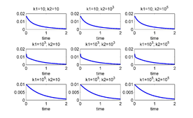
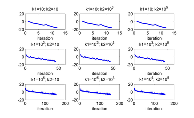
When controlling via two junctions only the case when using junctions 2 and 3 is a successful one (for all values of <math display="inline">k_1</math> and <math display="inline">k_2</math>). In Figures [[#img-7|7]] and [[#img-8|8]] are shown the respective results. | When controlling via two junctions only the case when using junctions 2 and 3 is a successful one (for all values of <math display="inline">k_1</math> and <math display="inline">k_2</math>). In Figures [[#img-7|7]] and [[#img-8|8]] are shown the respective results. | ||
| Line 1,649: | Line 1,679: | ||
|[[Image:Draft_LOPEZ_262416069-Ufigure7J23L16.png|276px|u<sup>∆t</sup> (top) and \| y<sup>∆t</sup>(⋅)\| (bottom) for several values of k₁ and k₂. The unstable equilibrium θ is given by \{ n₁,n₂,n₃\} =\{ 1,0,0(u)\} . The junctions used to control are 2 and 3.]] | |[[Image:Draft_LOPEZ_262416069-Ufigure7J23L16.png|276px|u<sup>∆t</sup> (top) and \| y<sup>∆t</sup>(⋅)\| (bottom) for several values of k₁ and k₂. The unstable equilibrium θ is given by \{ n₁,n₂,n₃\} =\{ 1,0,0(u)\} . The junctions used to control are 2 and 3.]] | ||
|- style="text-align: center; font-size: 75%;" | |- style="text-align: center; font-size: 75%;" | ||
| − | | colspan="2" | '''Figure 7:''' <math>\mathbf{u}^{\Delta t}</math> ( | + | | colspan="2" | '''Figure 7:''' <math>\mathbf{u}^{\Delta t}</math> (left) and <math>\| \mathbf{y}^{\Delta t}(\cdot )\| </math> (right) for several values of <math>k_1</math> and <math>k_2</math>. The unstable equilibrium <math>\boldsymbol{\theta }</math> is given by <math>\{ n_{1},n_{2},n_{3}\} =\{ 1,0,0(u)\} </math>. The junctions used to control are 2 and 3. |
|} | |} | ||
| Line 1,657: | Line 1,687: | ||
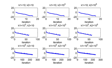
|[[Image:Draft_LOPEZ_262416069-Ufigure9J23L16.png|384px|ln\| g<sub>q</sub><sup>∆t</sup>\| for several values of k₁ and k₂. The unstable equilibrium θ is given by \{ n₁,n₂,n₃\} =\{ 1,0,0(u)\} . The junctions used to control are 2 and 3.]] | |[[Image:Draft_LOPEZ_262416069-Ufigure9J23L16.png|384px|ln\| g<sub>q</sub><sup>∆t</sup>\| for several values of k₁ and k₂. The unstable equilibrium θ is given by \{ n₁,n₂,n₃\} =\{ 1,0,0(u)\} . The junctions used to control are 2 and 3.]] | ||
|- style="text-align: center; font-size: 75%;" | |- style="text-align: center; font-size: 75%;" | ||
| − | | colspan="1" | '''Figure 8:''' <math> | + | | colspan="1" | '''Figure 8:''' <math>Ln\| \mathbf{g}_q^{\Delta t}\| </math> for several values of <math>k_1</math> and <math>k_2</math>. The unstable equilibrium <math>\boldsymbol{\theta }</math> is given by <math>\{ n_{1},n_{2},n_{3}\} =\{ 1,0,0(u)\} </math>. The junctions used to control are 2 and 3. |
|} | |} | ||
| − | === | + | ===4.2 Controlling via three junctions=== |
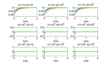
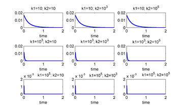
Figures [[#img-9|9]] and [[#img-10|10]] show the results when the three junctions are used to control. As we can see, for all values of the penalty parameters, the linear system is controlled. | Figures [[#img-9|9]] and [[#img-10|10]] show the results when the three junctions are used to control. As we can see, for all values of the penalty parameters, the linear system is controlled. | ||
| Line 1,670: | Line 1,700: | ||
|[[Image:Draft_LOPEZ_262416069-Ufigure10J123L16.png|360px|u<sup>∆t</sup> (top) and \| y<sup>∆t</sup>(⋅)\| (bottom) for several values of k₁ and k₂. The unstable equilibrium θ is given by \{ n₁,n₂,n₃\} =\{ 1,0,0(u)\} . The junctions used to control are 1, 2 and 3.]] | |[[Image:Draft_LOPEZ_262416069-Ufigure10J123L16.png|360px|u<sup>∆t</sup> (top) and \| y<sup>∆t</sup>(⋅)\| (bottom) for several values of k₁ and k₂. The unstable equilibrium θ is given by \{ n₁,n₂,n₃\} =\{ 1,0,0(u)\} . The junctions used to control are 1, 2 and 3.]] | ||
|- style="text-align: center; font-size: 75%;" | |- style="text-align: center; font-size: 75%;" | ||
| − | | colspan="2" | '''Figure 9:''' <math>\mathbf{u}^{\Delta t}</math> ( | + | | colspan="2" | '''Figure 9:''' <math>\mathbf{u}^{\Delta t}</math> (left) and <math>\| \mathbf{y}^{\Delta t}(\cdot )\| </math> (right) for several values of <math>k_1</math> and <math>k_2</math>. The unstable equilibrium <math>\boldsymbol{\theta }</math> is given by <math>\{ n_{1},n_{2},n_{3}\} =\{ 1,0,0(u)\} </math>. The junctions used to control are 1, 2 and 3. |
|} | |} | ||
| Line 1,678: | Line 1,708: | ||
|[[Image:Draft_LOPEZ_262416069-Ufigure12J123L16.png|384px|ln\| g<sub>q</sub><sup>∆t</sup>\| for several values of k₁ and k₂. The unstable equilibrium θ is given by \{ n₁,n₂,n₃\} =\{ 1,0,0(u)\} . The junctions used to control are 1, 2 and 3.]] | |[[Image:Draft_LOPEZ_262416069-Ufigure12J123L16.png|384px|ln\| g<sub>q</sub><sup>∆t</sup>\| for several values of k₁ and k₂. The unstable equilibrium θ is given by \{ n₁,n₂,n₃\} =\{ 1,0,0(u)\} . The junctions used to control are 1, 2 and 3.]] | ||
|- style="text-align: center; font-size: 75%;" | |- style="text-align: center; font-size: 75%;" | ||
| − | | colspan="1" | '''Figure 10:''' <math> | + | | colspan="1" | '''Figure 10:''' <math>Ln\| \mathbf{g}_q^{\Delta t}\| </math> for several values of <math>k_1</math> and <math>k_2</math>. The unstable equilibrium <math>\boldsymbol{\theta }</math> is given by <math>\{ n_{1},n_{2},n_{3}\} =\{ 1,0,0(u)\} </math>. The junctions used to control are 1, 2 and 3. |
|} | |} | ||
| Line 1,689: | Line 1,719: | ||
|[[Image:Draft_LOPEZ_262416069-Ufigure17t12L16.png|240px|Optimal controls for the linear system (top), and Euclidean norm of the controlled solution ϕ<sup>∆t</sup> of the nonlinear system (bottom).]] | |[[Image:Draft_LOPEZ_262416069-Ufigure17t12L16.png|240px|Optimal controls for the linear system (top), and Euclidean norm of the controlled solution ϕ<sup>∆t</sup> of the nonlinear system (bottom).]] | ||
|- style="text-align: center; font-size: 75%;" | |- style="text-align: center; font-size: 75%;" | ||
| − | | colspan="2" | '''Figure 11:''' Optimal controls | + | | colspan="2" | '''Figure 11:''' Optimal controls (left), and Euclidean norm of the controlled solution <math>\boldsymbol{\phi }^{\Delta t}</math> of the nonlinear system (right). |
|} | |} | ||
| Line 1,700: | Line 1,730: | ||
|[[Image:Draft_LOPEZ_262416069-Ufigure14J123L16.png|360px|Extended controlled solution y<sub>i</sub><sup>∆t</sup> of the linear perturbation model (top), and extended controlled solution ϕ<sub>i</sub><sup>∆t</sup> of the nonlinear system (bottom). After t=2 the controls are extended as cero.]] | |[[Image:Draft_LOPEZ_262416069-Ufigure14J123L16.png|360px|Extended controlled solution y<sub>i</sub><sup>∆t</sup> of the linear perturbation model (top), and extended controlled solution ϕ<sub>i</sub><sup>∆t</sup> of the nonlinear system (bottom). After t=2 the controls are extended as cero.]] | ||
|- style="text-align: center; font-size: 75%;" | |- style="text-align: center; font-size: 75%;" | ||
| − | | colspan="2" | '''Figure 12:''' Extended controlled solution <math>y_i^{\Delta t}</math> of the linear perturbation model ( | + | | colspan="2" | '''Figure 12:''' Extended controlled solution <math>y_i^{\Delta t}</math> of the linear perturbation model (left), and extended controlled solution <math>\phi _i^{\Delta t}</math> of the nonlinear system (right). After <math>t=2</math> the controls are extended as cero. |
|} | |} | ||
| − | === | + | ===4.3 Controlling via three junctions in the interval [0,20]=== |
To control during the whole time interval <math display="inline">(0,20)</math> we have divided the time interval into subintervals of smaller length <math display="inline">\Delta T = T/Q=2</math>, and we denote <math display="inline">q\Delta T</math> by <math display="inline">T_q</math> for <math display="inline">q = 1, . . .,Q</math>; we proceed then as follows: | To control during the whole time interval <math display="inline">(0,20)</math> we have divided the time interval into subintervals of smaller length <math display="inline">\Delta T = T/Q=2</math>, and we denote <math display="inline">q\Delta T</math> by <math display="inline">T_q</math> for <math display="inline">q = 1, . . .,Q</math>; we proceed then as follows: | ||
| Line 1,711: | Line 1,741: | ||
* We do <math display="inline">q = q + 1</math> and we repeat the process. | * We do <math display="inline">q = q + 1</math> and we repeat the process. | ||
| − | The above time partitioning method has been applied with <math display="inline">\boldsymbol{\phi }_0=\boldsymbol{\theta }+\delta \boldsymbol{\theta }</math> and <math display="inline">\delta \boldsymbol{\theta }=[1e-2,1e-2,1e-2]</math>, the time interval under consideration being <math display="inline">[0,20]</math>; we have used <math display="inline">\Delta T = 2.0</math>. After <math display="inline">t = 20</math>, we have taken <math display="inline">\mathbf{v = 0}</math> in ([[#eq-9|9]]) and in ([[#eq-5|5]]) to observe the evolution of the suddenly uncontrolled linear and nonlinear systems. The results are reported in Figure [[#img-13|13]]. We observe that the system is practically stabilized for <math display="inline">1 \leq t \leq 20</math>, but if one stops controlling, the small residual perturbations of the system at <math display="inline">t = 20</math>, are sufficient to destabilize the linear and nonlinear systems and induces the nonlinear one to transition to a stable equilibrium in finite time. | + | The above time partitioning method has been applied with <math display="inline">\boldsymbol{\phi }_0=\boldsymbol{\theta }+\delta \boldsymbol{\theta }</math> and <math display="inline">\delta \boldsymbol{\theta }=[1e-2,1e-2,1e-2]</math>, the time interval under consideration being <math display="inline">[0,20]</math>; we have used <math display="inline">\Delta T = 2.0</math>. After <math display="inline">t = 20</math>, we have taken <math display="inline">\mathbf{v} = \mathbf{0}</math> in ([[#eq-9|9]]) and in ([[#eq-5|5]]) to observe the evolution of the suddenly uncontrolled linear and nonlinear systems. The results are reported in Figure [[#img-13|13]]. We observe that the system is practically stabilized for <math display="inline">1 \leq t \leq 20</math>, but if one stops controlling, the small residual perturbations of the system at <math display="inline">t = 20</math>, are sufficient to destabilize the linear and nonlinear systems and induces the nonlinear one to transition to a stable equilibrium in finite time. |
<div id='img-13'></div> | <div id='img-13'></div> | ||
| Line 1,721: | Line 1,751: | ||
| colspan="2"|[[Image:Draft_LOPEZ_262416069-Ufigure20t28L16.png|300px|Controls calculated each two seconds (top); Euclidean norm of the controlled solution y<sup>∆t</sup> using the controls in the top (middle); Euclidean norm of the controlled solution ϕ<sup>∆t</sup> using the controls in the top (bottom).]] | | colspan="2"|[[Image:Draft_LOPEZ_262416069-Ufigure20t28L16.png|300px|Controls calculated each two seconds (top); Euclidean norm of the controlled solution y<sup>∆t</sup> using the controls in the top (middle); Euclidean norm of the controlled solution ϕ<sup>∆t</sup> using the controls in the top (bottom).]] | ||
|- style="text-align: center; font-size: 75%;" | |- style="text-align: center; font-size: 75%;" | ||
| − | | colspan="2" | '''Figure 13:''' Controls calculated each two seconds (top); Euclidean norm of the controlled solution <math>\mathbf{y}^{\Delta t}</math> using the controls in the top ( | + | | colspan="2" | '''Figure 13:''' Controls calculated each two seconds (top-left); Euclidean norm of the controlled solution <math>\mathbf{y}^{\Delta t}</math> using the controls in the top (top-right); Euclidean norm of the controlled solution <math>\boldsymbol{\phi }^{\Delta t}</math> using the controls in the top-left (bottom). |
|} | |} | ||
| − | == | + | ==5 Conclusions== |
We have stabilized the phases of a JJAM model, around an unstable equilibrium by using the classical approach: linearize the state model around the unstable equilibrium; control the linear model in order to stabilize it around the unstable equilibrium; apply the linear control to the nonlinear model and hope this control will also stabilize it. Since the time interval is large (<math display="inline">t\in [0, 30]</math>) in certain applications, and could be that the linear control do not stabilize the nonlinear model, we subdivi-ded the original interval into subintervals and calculate iteratively the linear control on each subinterval, obtaining a piecewise control that stabilize not only the linear model but also the nonlinear one. For an efficient calculation of the control we formulated an operational linear equation satisfied by the control. The associated operator is self-adjoint and elliptic, so a conjugate gradient algorithm for quadratic functional was used. | We have stabilized the phases of a JJAM model, around an unstable equilibrium by using the classical approach: linearize the state model around the unstable equilibrium; control the linear model in order to stabilize it around the unstable equilibrium; apply the linear control to the nonlinear model and hope this control will also stabilize it. Since the time interval is large (<math display="inline">t\in [0, 30]</math>) in certain applications, and could be that the linear control do not stabilize the nonlinear model, we subdivi-ded the original interval into subintervals and calculate iteratively the linear control on each subinterval, obtaining a piecewise control that stabilize not only the linear model but also the nonlinear one. For an efficient calculation of the control we formulated an operational linear equation satisfied by the control. The associated operator is self-adjoint and elliptic, so a conjugate gradient algorithm for quadratic functional was used. | ||
Latest revision as of 00:54, 24 December 2022
Abstract
In this paper we consider a system of three nonlinear ordinary differential equations that model a three Josephson Junctions Array (JJA). Our goal is to stabilize the system around an unstable equilibrium employing an optimal control approach. We first define the cost functional and calculate its differential by using perturbation analysis and variational calculus. For the computational solution of the optimality system we consider a conjugate gradient algorithm for quadratic functionals in Hilbert spaces, combined with a finite difference discretization of the involucrated differential equations.
Key word: Josephson Junction, Cryogenic Memory, Conjugate Gradient Algorithms, Stabilization, Optimal Control.
MSC[2010] 65K10, 49M25.
1 Introduction
In this article we discuss the numerical simulation of a control approach to stabilize a Josephson Junction Array (JJA) around an unstable steady state. Our methodology relies significantly on a conjugate gradient algorithm operating in a well-chosen control space. It has been shown recently that such an array can carry out the functions of a memory cell operations ([1,2,3,4,5]), consequently this array is frequently referred as a Josephson junction array memory (JJAM).
A Josephson junction is a quantum interference device that consists of two super-conductors coupled by a weak link that may be, for example, an insulator or a ferromagnetic material. A Josephson junction can carry current without resistance (this current is called supercurrent) and such a device is an example of a macroscopic quantum phenomenon. In 1962, B.D. Josephson proposed the equations governing the dynamics of the Josephson junction effect, namely:
|
|
(1) |
where , being the Planck constant, is the electric charge of the electron, and are the voltage and current across the junction, respectively, is the phase difference across the junction, and, finally, the constant is the critical current across the junction. The Josephson junction technology offers numerous applications and could potentially provide sound alternatives for computer memory devices. In a 2005 US National Security Agency (NSA) report it has been alluded that, as transistors were rapidly approaching their physical limits, their most likely successors would be cryogenic devices based on Josephson junctions [6]. Indeed, (cf. [7]), ``Single flux quantum (SFQ) circuits produce small current pulses that travel at about the speed of light. Superconducting passive transmission lines (PTL) are also able to transmit the pulses with extremely low losses". These are currently the fastest switching digital circuits, since (cf. [8]) ``Josephson junctions, the superconducting switching devices, switch quickly ( ps), dissipate very little energy per switch (), and communicate information via current pulses that propagate over superconducting transmission lines nearly without loss". Recently it was suggested that a small array consisting of inductively coupled Josephson junctions possesses all the basic functions (WRITE, READ, RESET) of a memory cell ([1], [3] and the references therein). In the two above articles, stable zero-voltage states were identified and basic memory cell operations based on the transitions between the equilibrium states were identified.
The equations modeling the dynamics of the inductively coupled Josephson junction array can be written in the following dimensionless form ( corresponds to )
|
|
(2) |
where , being a direct current and an additional energy as a current pulse. Plausible values for the various quantities in the model are:
|
For those regimes where the second order derivatives can be neglected (meaning the junctions are (relatively) highly dissipative), (2) reduces to
|
|
(5) |
The Read/Write operations can be performed by applying appropriate Gaussian pulses ([1], [4], [5] ) in order to drive the system from an equilibrium configuration to another one. In [9], we went beyond Gaussian pulses and investigated an optimal controllability approach in to perform these transitions between equilibrium configurations. These approach is closely related to the methodology discussed in [10] for systems modelled by partial differential equations.
For the driving currents and coupling parameters provided in (3) and (4), the ordinary differential equation systems (5) (and (2) with ) have several steady state solutions, consisting of phase triplets. In many cases, the steady state phases are near the values , for certain integers , and, according to Braiman, et. al., ([1]), equilibrium junction phases can be defined by their offsets from the negative cosine function's minima, as shown in the following equation
|
|
(6) |
Following Braiman et al., ([1]), Table 1 includes all the possible triplets of stable steady state offsets, where . For the steady states, we assumed, without loss of generality, that , since all the phases can be shifted by the same multiple of . Also we include in Table 1 three unstable steady states, namely: . Here the description of some unstable equilibria is artificial (in the sense that the terms are not small and its only purpose is to be consistent with the description of stable states).
| no | stable | equil | ||||||
| no | stable | equil | ||||||
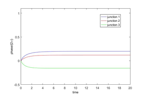
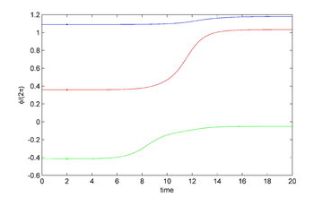
For the set of dc currents and coupling parameters defined by (3) and (4), no stable steady state exists when the first junction phase is about (respectively ) greater than both of the other two junction phases (see row where (respectively )). Following Braiman, et. al., [1], for memory cell demonstration it is sufficient to manipulate the system within the particular sets of states, namely states and . The circuit of three coupled Rapid Single Joint (RSJ) unit circuits associated with model (5) can operate as a memory cell if a set of operators can transition the system to clearly defined states and can output a signal that discriminates memory states. The value as presented in equation (6), will describe the location of the junction phase. When all three junction phases are in the same sinusoidal potential well, the system will be considered in the `0' state, When the phases of the first and second junctions are shifted to the next potential well (about greater), the cell will be in the `1' state, . These two states correspond to the first and third rows of Table 1. Figure 1 shows the phases of the junctions when the systems starts from zero initial conditions. The junctions settle into the steady state `0' where all phases are close to the same multiple of . For convenience, in several of the following figures the phases are normalized by and in all the graphs that include different colors, color blue, red and green is associated with junction 1, 2 and 3, respectively.
|
| Figure 1: Time series of the phases scaled by , with zero initial conditions. |
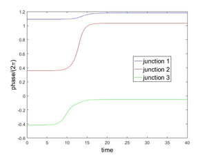
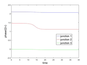
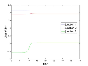
In this work we investigate a controllability approach in order to stabilize the phase junctions of (5) around an unstable equilibrium. Figures 2 and 3 show the behavior of the system when the initial conditions are approximations of the unstable equilibrium =, , .
|
|
| Figure 2: Evolution to state (left), (right) from an approximation to the unstable equilibrium (left), (right). | |
|
| Figure 3: Evolution to from an approximation to the unstable equilibrium . |
The organization of this paper is as follows. In Section 2 we focus on a methodology to stabilize the JJAM system around an unstable equilibrium configuration, via a controllability approach. Section 3 is concerning the practical aspects of this methodology. In Section 4 we show the numerical results and in Section 5 we give the conclusions.
2 Formulation of the optimal control problem for the stabilization of the JJAM and the conjugate gradient algorithm
2.1 The approach
As we explained in the Introduction, Figures 2 and 3 show the behavior of the system (5) when the initial conditions are approximations of the unstable equilibrium configurations = , , . Our goal in this subsection is to stabilize the system (5), around an unstable equilibrium, controlling it via one, two or three junctions i.e., we want to maintain the phase values in Figures 2 and 3 almost constant along time. This constant value must be the initial value on each case. The approach taken here is the following classical one, namely,
(a) Linearize the model (5) in the neighborhood of an (unstable) equilibrium of the system.
(b) Compute an optimal control for the linearized model.
(c) Apply the above control to the nonlinear system.
Let us consider an unstable state of (5) and a small initial variation of . The perturbation of the steady-state in satisfies approximately the following linear model
|
|
(7) |
At least one of the eigenvalues of the jacobian of system (7) is positive. This means that the system can develop blow up phenomena (in infinite time). Figures 4, 5 and 6 show the solution of (7) for the three unstable equilibriums given by in Table 1, respectively. The used value for the initial perturbation was .
![Solution y=δϕ of (7) for the unstable equilibrium given by \{ n₁,n₂,n₃\} =\{ 1,0,0(u)\} and δθ=[ 1e-2, 1e-2, 1e-2].](/wd/images/thumb/8/81/Draft_LOPEZ_262416069-Ufigure1.png/280px-Draft_LOPEZ_262416069-Ufigure1.png)
|
| Figure 4: Solution of (7) for the unstable equilibrium given by and . |
![Solution y=δϕ of (7) for the unstable equilibrium given by \{ n₁,n₂,n₃\} =\{ 2,1,0(u)\} and δθ=[ 1e-2, 1e-2, 1e-2].](/wd/images/thumb/b/be/Draft_LOPEZ_262416069-Ufigure2.png/280px-Draft_LOPEZ_262416069-Ufigure2.png)
|
| Figure 5: Solution of (7) for the unstable equilibrium given by and . |
![Solution y=δϕ of (7) for the unstable equilibrium given by \{ n₁,n₂,n₃\} =\{ 2,2,0(u)\} and δθ=[ 1e-2, 1e-2, 1e-2].](/wd/images/thumb/7/78/Draft_LOPEZ_262416069-Ufigure3.png/280px-Draft_LOPEZ_262416069-Ufigure3.png)
|
| Figure 6: Solution of (7) for the unstable equilibrium given by and . |
It is clear that the model (7) is no longer valid if becomes too large but the idea behind considering the linearized model (7) is to use it to compute a control action preventing from becoming too large (and possibly driving to zero) and hope that the computed control will also stabilize the original nonlinear system (5) with initial condition
|
|
(8) |
2.2 The Linear Control Problem
Using the notation , we shall (try to) stabilize the controlled variant of system (7) (the three junctions are used to control):
|
|
(9) |
via the following control formulation:
|
|
(10) |
where
|
|
(11) |
and .
2.3 Optimality Conditions and Conjugate Gradient Solution for Problem (10)
2.3.1 Generalities and Synopsis
Let us denote by the differential of at . Since is a Hilbert Space for the scalar product defined by
|
|
the action of on can also be written as
|
|
with . If is the solution of problem (10), it is characterized [from convexity arguments (see, e.g., [11])] by
|
|
(12) |
Since the cost function is quadratic and since the state model (7) is linear, is in fact an affine function of , implying in turn from (12) that is the solution of a linear equation in the control space . In abstract form, equation (12) can be written as
|
|
and from the properties (need to be shown) of the operator , problem could be solved by a (quadratic case)-conjugate gradient algorithm operating in the space . The practical implementation of the above algorithm would requires the explicit knowledge of .
2.3.2 Computing DJ(v)
We compute the differential of the cost function at assumming that . To achieve that goal we will use a perturbation analysis. Let us consider thus a perturbation of the control variable . We have then,
|
|
(13) |
where in (13):
(i) We denote by ab the dot product of two vectors a and b.
(ii) The function is the solution of the following initial value problem, obtained by perturbation of (9):
|
|
(14) |
where , In matrix-vector form (14) reads as follows:
|
|
(15) |
where and are diagonal matrices with coefficients and , , respectively, and
|
|
We introduce now a vector-valued function that we assume differentiable over ; multiplying by both sides of the differential equation in (15), and integrating over we obtain, after integrating by parts, and taking into account the symmetry of the matrices and , the following equation
|
|
(16) |
Now suppose that the vector-valued function is solution of the following (adjoint system):
|
|
(17) |
It follows from (16), (17) that
|
|
(18) |
Combining (13) and (18) we obtain that
|
|
(19) |
which implies in turn that
|
|
(20) |
Remark 1. So far, we have been assuming that a control is acting on the -th junction. The method we used to compute would still apply if one considers controlling the transition from to using only one or only two controls. The same apply for the results in the next sections
2.3.3 Optimality conditions for problem (10)
Let be the solution of problem (10) and let us denote by (respectively, ) the corresponding solution of the state system (9) (respectively, of the adjoint system (17)). It follows from Subsubsection 3.3.2 that is equivalent to the following (optimality) system:
|
Conversely, it can be shown (see, e.g., [11]) that the system (21)–(25) characterizes as the solution (necessarily unique here) of the control problem (10). The optimality conditions (21)–(25) will play a crucial role concerning the iterative solution of the control problem (10).
2.3.4 Functional equations satisfied by the optimal control
Our goal here is to show that the optimality condition can also be written as
|
|
(26) |
where the linear operator is a strongly elliptic and symmetric isomorphism from into itself (an automorphism of and where . A candidate for is the linear operator from into itself defined by
|
|
where is obtained from via the successive solution of the following two problems:
|
|
(27) |
which is forward in time, and the adjoint system (17) in which is backward in time. To see that operator is a symmetric and strongly elliptic isomorphism from into itself consider , belonging to and define , by
|
|
we have then
|
|
(28) |
On the other hand, we have, starting with the differential equation in (27) and using integration by parts, that
|
|
This implies that
|
|
(29) |
Combining (28) with (29) we obtain
|
|
(30) |
Relation (30) imply the symmetry of ; we also have
|
|
which implies the strong ellipticity of over . The linear operator , being continuous and strongly elliptic over , is an automorphism of . To identify the right hand side of equation (26), we introduce and defined as the solutions of
|
|
(31) |
and
|
|
(32) |
Suppose now that and satisfies the optimality conditions. Define
|
|
Subtracting (31) and (32) from (27) and (17) we obtain
|
|
(33) |
and
|
|
(34) |
From the definition of operator it follows that
|
|
(35) |
the right hand side of (35) is the vector that we were looking for.
From the properties of , problem (35) can be solved by a conjugate gradient algorithm operating in the Hilbert space . This algorithm will be described in the following subsubsection.
2.3.5 Conjugate gradient solution of the control problem (10)
Problem (35) can be written in variational form as
|
|
(36) |
From the symmetry and -ellipticity of the bilinear form
|
|
the variational problem (36) is a particular case of the following class of linear variational problems:
|
|
(37) |
where
(i) is a real Hilbert space for the scalar product and the correspondent norm
(ii) : is bilinear, continuous, symmetric and -elliptic, i.e., such that ;
(iii) : is linear and continuous.
If the above properties hold, then problem (37) has a unique solution (see [10]); in fact, the symmetry of is not necessary in order to have a unique solution to problem (37); however, the symmetry of , combined with the other properties, allows problem (37) to be solved by the following conjugate gradient algorithm:
- Step 1. is given.
- Step 2. Solve
|
|
(38) |
and set
|
|
(39) |
- Step 3. For , , and being known, compute , and as follows:
|
|
(40) |
and take
|
|
(41) |
Solve
|
|
(42) |
and compute
|
|
(43) |
|
|
(44) |
- Step 4. Do n=n+1 and go to (40).
Let us recall that is a Hilbert space for the inner-product and the associated norm , implying that problem (10)-(36) can be solved applying the conjugate gradient algorithm (38)-(44). The above algorithm takes the following form:
- Suppose
|
|
(45) |
- Solve
|
|
(46) |
and then
|
|
(47) |
- Set
|
|
(48) |
- If take ; otherwise, set
|
|
(49) |
For , , and being known, we compute and if necessary, as follows:
- Solve
|
|
(50) |
and then
|
|
(51) |
Set
|
|
(52) |
and
|
|
(53) |
- Set
|
|
(54) |
- Set
|
|
(55) |
- If take ; otherwise, compute
|
|
(56) |
and set
|
|
(57) |
- Do and return to (50) .
- End of algorithm.
The state variable can be actualized simultaneously with the control since for all we have
|
|
(58) |
so,
|
|
(59) |
which, by definition of implies that
|
|
The practical implementation of algorithm (45)-(57), via a finite difference discretization of problem (10), will be discussed in the following section.
3 Discrete formulation of the optimal control problem
3.1 Finite difference approximation of problem (10)
We approximate (10) when by
|
|
(60) |
where:
- with a "large" positive integer.
The cost functional is defined by
|
|
with and obtained from and via the following discrete variant of (9):
|
|
(61) |
and for
|
|
(62) |
To compute we have thus to solve a linear system of the following type:
|
|
(63) |
The matrix being a matrix symmetric and positive definite, solving (63) is easy.
3.2 Optimality Conditions and conjugate gradient solution of (60)
3.2.1 Computing DJ∆t(v)
Assuming that one wants to use the conjugate gradient algorithm (38)-(44) to solve the discrete problem (60), we compute first . On we will use the following inner-product
|
|
We have
|
|
(64) |
with obtained by perturbation of (61), (62), that is
|
|
(65) |
and for
|
|
(66) |
Let us introduce Taking the dot product of with each side of equation (66), we obtain after summation and multiplication by
|
|
(67) |
Applying a discrete integration by parts to relation (67), and considering that we obtain:
|
|
(68) |
or equivalently
|
|
(69) |
Suppose that verifies the following discrete adjoint system:
|
|
(70) |
and for
|
|
(71) |
It follows from (64), (69)-(71) that
|
|
(72) |
that is
|
|
(73) |
3.2.2 Optimality conditions for (60)
The optimality conditions for the discrete problem (60) are
|
3.2.3 Functional equation for the discrete control solution of (60)
Following the sketch for the continuous case we can show that the discrete version of operator and the discrete version of satisfies the equation
|
|
(79) |
where is the discrete control satisfying the optimality condition (74). Operator enjoys the same properties than the continuous version: symmetric, strongly elliptic and continuous, allowing us to use a conjugate gradient like (38)-(44) to solve (79).
3.2.4 Conjugate gradient solution of the discrete control problem (60)
Using to denote the discrete value of the vector-valued function at time and iteration ; similarly, will denote the discrete value of the control at time and iteration , the conjugate gradient algorithm (38)-(44) to solve the finite dimensional problem (60) reads as follow:
- Suppose
|
|
(80) |
- Compute and via the solution of
|
|
(81) |
and then
|
|
(82) |
- Set
|
|
(83) |
- If
|
|
take ; otherwise, set
|
|
(84) |
For , , and being known, the last two different from , we compute , and, if necessary as follows:
- Solve
|
|
(85) |
and then
|
|
(86) |
Set
|
|
(87) |
and
|
|
(88) |
- Compute
|
|
(89) |
and
|
|
(90) |
- If
|
|
take ; otherwise, compute
|
|
(91) |
and set
|
|
(92) |
- Do and return to (85) .
- End of algorithm
Similar to the continuous case, we can deduce that if then
|
|
4 Numerical Results
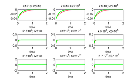
In previous sections we have described a methodology and the respective practical algorithms to use a control on each joint in order to stabilize the linear JJAM perturbation system around an unstable equilibrium. It is easy to simplify the procedure and algorithm to the case when we want to control via only (any combina-tion of) two junctions or via only one junction. However, since (according to the experiments) it is necessary to control via at least two junctions in order to stabilize the system around an unstable equilibrium, we show only the results when two and three junctions are used to control the system model. For the calculations we used for the stopping criteria in conjugate gradient algorithm, and for solving the differential systems. In the next two subsections we use as the equilibrium given by and ; the time interval under consideration being . Finally we apply iteratively this control process to stabilize in the longer interval using 10 subintervals of length 2.
4.1 Controlling via two junctions
When controlling via two junctions only the case when using junctions 2 and 3 is a successful one (for all values of and ). In Figures 7 and 8 are shown the respective results.
|
|
| Figure 7: (left) and (right) for several values of and . The unstable equilibrium is given by . The junctions used to control are 2 and 3. | |
|
| Figure 8: for several values of and . The unstable equilibrium is given by . The junctions used to control are 2 and 3. |
4.2 Controlling via three junctions
Figures 9 and 10 show the results when the three junctions are used to control. As we can see, for all values of the penalty parameters, the linear system is controlled.
|
|
| Figure 9: (left) and (right) for several values of and . The unstable equilibrium is given by . The junctions used to control are 1, 2 and 3. | |
|
| Figure 10: for several values of and . The unstable equilibrium is given by . The junctions used to control are 1, 2 and 3. |
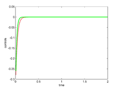
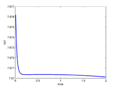
For the particular values and of the penalty parameters we show in Figure 11 the controls and the norm of the solution of the nonlinear system (the behavior of the solution of the linear system is shown in Figure 9)
|
|
| Figure 11: Optimal controls (left), and Euclidean norm of the controlled solution of the nonlinear system (right). | |
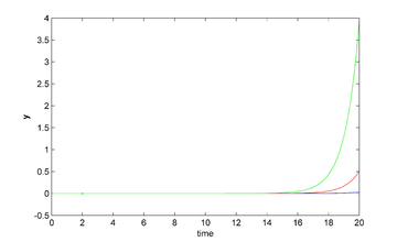
In Figure 12 we show the solution for the linear and nonlinear model, using controls in Figure 11 (we continue from to with no control).
|
|
| Figure 12: Extended controlled solution of the linear perturbation model (left), and extended controlled solution of the nonlinear system (right). After the controls are extended as cero. | |
4.3 Controlling via three junctions in the interval [0,20]
To control during the whole time interval we have divided the time interval into subintervals of smaller length , and we denote by for ; we proceed then as follows:
- For , we denote by the difference , and we solve the associated linear control problem (9)-(11) in ; let us denote by the corresponding control. This control is injected in (5) with initial condition (8) and , and we denote by the difference .
- For , we denote by the difference ; we solve the associated linear control problem (9)-(11) in , with replaced by , and we denote by the corresponding optimal control. The control is injected in (5) with initial condition (8) and , and we denote by the difference .
- We do and we repeat the process.
The above time partitioning method has been applied with and , the time interval under consideration being ; we have used . After , we have taken in (9) and in (5) to observe the evolution of the suddenly uncontrolled linear and nonlinear systems. The results are reported in Figure 13. We observe that the system is practically stabilized for , but if one stops controlling, the small residual perturbations of the system at , are sufficient to destabilize the linear and nonlinear systems and induces the nonlinear one to transition to a stable equilibrium in finite time.
5 Conclusions
We have stabilized the phases of a JJAM model, around an unstable equilibrium by using the classical approach: linearize the state model around the unstable equilibrium; control the linear model in order to stabilize it around the unstable equilibrium; apply the linear control to the nonlinear model and hope this control will also stabilize it. Since the time interval is large () in certain applications, and could be that the linear control do not stabilize the nonlinear model, we subdivi-ded the original interval into subintervals and calculate iteratively the linear control on each subinterval, obtaining a piecewise control that stabilize not only the linear model but also the nonlinear one. For an efficient calculation of the control we formulated an operational linear equation satisfied by the control. The associated operator is self-adjoint and elliptic, so a conjugate gradient algorithm for quadratic functional was used.
BIBLIOGRAPHY
[1] Y. Braiman, B. Neschke, N. Nair, N. Ima, and R. Glowinski. (2016) Memory States in Small Arrays of Josephson Junctions, PHYSICAL REVIEW E (94), 052223: 1-13.
[2] Y. Braiman and N. Nair and J. Rezac and N. Imam. (2016) Memory Cell Operation Based on Small Josephson Junction Arrays, Superconductor Science and Technology (129), 124003: 1-15.
[3] J.D. Rezac and N. Imam and Y. Braiman. (2017) Parameter optimization for transitions between memory states in small arrays of Josephson junctions, PHYSICA A (474), 267-281.
[4] Harvey, Roland and Qu, Zhihua. (2018) Control of Cryogenic Memory State Transitions in a Josephson Junction Array, 2018 Annual American Control Conference (ACC), 5671-5676.
[5] N. Nair and Y. Braiman. (2018) A Ternary Memory Cell Using Small Josephson Junction Arrays, Superconductor Science and Technology (31).
[6] F. Bedard and N. Welker and G. R. Cotter and M. A. Escavage and J. T. Pinkston. (2005) Superconducting Technology Assessment, National Security Agency, Office of Corporate Assessment, url = https://www.nitrd.gov/pubs/nsa/sta.pdf.
[7] F. A. Holmes and L. Ripple and M. A. Manheimer. (2013) Energy-Efficient Superconducting Computing-Power Budgets and Requirements, IEEE Transactions on Applied Superconductivity , 23 (3).
[8] IARPA. (2013) Broad Agency Announcement: IARPA-BAA-13-05, Cryogenic Computing Complexity (C3) Program, IARPA.
[9] Roland Glowinski and Jorge López and Héctor Juárez and Yehuda Braiman. (2020) On the controllability of transitions between equilibrium states in small inductively coupled arrays of Josephson junctions: A computational approach, Journal of Computational Physics (403), 109023, doi = https://doi.org/10.1016/j.jcp.2019.109023, url = http://www.sciencedirect.com/science/article/pii/S0021999119307296.
[10] R. Glowinski and J.L. Lions and J. W. He. (2008) Exact and Approximate Controllability for Distributed Parameter Systems, Cambridge University Press, Cambridge, UK.
[11] J. L. Lions. (1971) Optimal Control of Systems Governed by Partial Differential Equations, Springer Verlag, New York.
Document information
Published on 16/11/22
Submitted on 09/09/22
Licence: CC BY-NC-SA license
Share this document
Keywords
claim authorship
Are you one of the authors of this document?
