(Created page with "== Abstract == In the last decades, the improvements in terms of computational power provides the capability to analyze with more detail the materials behavior. On one hand,...") |
|||
| (3 intermediate revisions by 2 users not shown) | |||
| Line 1: | Line 1: | ||
| − | == | + | ==1 Introduction== |
| − | + | Nowadays, numerous materials used in engineering industrial field, as well as in biological and biomedical area, are characterized by two or more constituents, also called phases. | |
| − | + | ||
| − | + | ||
| − | == Full | + | Carbon fiber composites, polycrystalline structures, concrete, bone or wood are only some examples of components where the constituents could be distinguished at certain length scale. These materials are called inhomogeneous. The length scale as well as the type of constituents are only some example of possible criterion to classify them. Indeed, microstructure take an important role during the analysis of the material because of the topology and the properties of each phase that determines its behavior. |
| − | < | + | |
| + | It is also possible to say that defining a microscale structure means to study the behavior of each phase in order to determine the overall behavior of the global structure in terms of physical properties such as mechanical, thermal, electrical, etc. | ||
| + | |||
| + | Geometry, structure, properties and behavior of the inhomogeneous materials could be separated in two different fields depending on its length scale. On one hand, the microscale (or fine-scale) corresponds to the microstructure where each phase is distinguishable. On the other hand, the macroscale (or coarse-scale) is the largest scale (and length) of the model, in contrast to the microscale that represents the lowest scale. | ||
| + | |||
| + | The most important assumption that has to be made when studying the micromechanical models is the scale separation between micro and macro structures. That assumption allows to separate the contribution of the microscale, defined as fluctuation part, from the macroscale ones, the constant part. | ||
| + | |||
| + | As it is explained in Bohm [1] these two contributions can be distinguished as fast and slow variables, where the fast variables, microscale fluctuations, can influence the behavior of the macroscale only through their volume average. Instead, the slow variables, the macroscale contribution, are not significant at the microscale level and can be considered as locally constant. | ||
| + | |||
| + | Otero et al. [2] and Petracca et al. [3], also provides an efficient multiscale strategy that, in case of first-order homogenization (FE2), ensures the macro and micro mesh independence taking into account the conservation of the energy dissipation of through the scales. | ||
| + | |||
| + | ==2 Multiscale Methods== | ||
| + | |||
| + | One of the most popular multiscale methods is the first-order homogenization. In this procedure, the strain obtained when analyzing the macroscopic structure is used to define the boundary conditions, applied on a Representative Volume Element RVE, to solve the Boundary Value Problem (BVP) at the microscale. | ||
| + | |||
| + | The basic principles of homogenization method were provided by Suquet [4] to obtain the constitutive equation for the homogenized properties of a heterogeneous material. The unit cell is defined as a microscopic subregion that is representative of the entire microstructure in an average sense. The RVE is employed to obtain the effective properties for the homogenized material because it is assumed that it must contain a sufficient number of heterogeneities [5] [6]. | ||
| + | |||
| + | The solution of the problem at the microscale, under such conditions, acts as an equivalent constitutive law for the macroscale, and it provides material stiffness and stresses as the volume average of the microscopic ones. This equivalent constitutive law is used in all the integration points of the macroscopic model to obtain the global response of the structure. When dealing with nonlinear microstructures, it will lead to an iterative procedure in which the RVE must be solved for different boundary conditions until both scales reach equilibrium, ensuring consistency between the micro- and macroscale solutions. | ||
| + | |||
| + | The first-order homogenization technique developed assumes a scale separation between the macro and the microscale, that is, the characteristic length of the microscale should be much smaller than the length of the macroscale elements, L: l<<L [7]. | ||
| + | |||
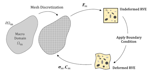
| + | The main steps of the classical FE2 technique can be resumed in the figure below. On each integration point of the discretized macroscale domain, the macroscopic strain tensor provides the input variables for the microscale domain. Then, the solution of the microscopic behavior of the RVE provides the macroscopic output and properties of the equivalent homogeneous medium. | ||
| + | |||
| + | <div class="center" style="width: auto; margin-left: auto; margin-right: auto;"> | ||
| + | [[Image:Zaghi_et_al_2021a-image5.png|486px]] </div> | ||
| + | |||
| + | <div class="center" style="width: auto; margin-left: auto; margin-right: auto;"> | ||
| + | <span style="text-align: center; font-size: 75%;">'''Figure 1.''' Representative homogenization scheme.</span></div> | ||
| + | |||
| + | In this paper, for the sake of simplicity, the procedure assumes small displacements and a quasi-static behavior in both macro and micro scales. However, the methodology proposed can be extended to other cases. | ||
| + | |||
| + | ==3 Discrete Multiscale Threshold Surface (DMTS) and Discrete Multiscale Constitutive Model (DMCM)== | ||
| + | |||
| + | The purpose of this paper is to provide two multiscale optimization techniques, directly derived from the classical first order multiscale theory. Considering these two methods, the main hypothesis is to construct a stress-strain state collector based on multiple RVE simulations able to describe the microscale behavior. Using an Equivalent Damage Parameter ( <math display="inline">{d}_{eq}</math>), index of the difference between the real and the elastic stress, the Discrete Multiscale Threshold Surface (DMTS) will identify with a finite number of points within the strain space the initiation of the non-linearity of the RVE. The DMTS is intended to reduce the computational cost of FE2, by identifying, during the analysis, where the RVE generation is needed and where the homogenized elastic properties are sufficient to obtain the macroscale response. As an extension of the DMTS, the Discrete Multiscale Constitutive Model (DMCM) aims to describe the complete behavior of the microstructure identifying multiple threshold surfaces related to increasing levels of <math display="inline">{d}_{eq}</math> decoupling the analysis from the FE2 methods. | ||
| + | |||
| + | Below, the authors will describe in detail all the aspects of both methods, providing examples and algorithms used for the numerical implementation. | ||
| + | |||
| + | ==='''3.1''' Strain database definition=== | ||
| + | |||
| + | In general, due to the complexity of the RVE, we cannot know a-priori the real stress behavior of the microscale. To overcome this problem, we will study the strain space doing a preliminary analysis of the RVE for different loading cases storing the stress response of the structure. These strains, defined as ''strain histories'', are in the multidimensional spaces <math display="inline">({\epsilon }_{xx},{\epsilon }_{yy},{\gamma }_{xy})</math> for 2D or <math display="inline">({\epsilon }_{xx},{\epsilon }_{yy},{\epsilon }_{zz},{\gamma }_{xy},{\gamma }_{yz},{\gamma }_{xz})</math> for 3D mechanical problems. | ||
| + | |||
| + | To make accessible this information during the analysis we will store the strain histories in a Homogenized Strain Database. In this chapter, for simplicity, we will only describe the 2D case, but it is perfectly extendable to 3D. | ||
| + | |||
| + | To obtain a complete definition of the microscale behavior we will impose as strain histories the value of evenly spaced point projected on the sphere of unitary radius centered in the origin of the axes <math display="inline">({\epsilon }_{xx},{\epsilon }_{yy},{\gamma }_{xy})</math>. We can uniquely define these points in 3D spherical coordinates system as the combination of three parameters ( <math display="inline">\theta ,\varphi ,\lambda</math> ), as we can see in the Figure 2, where the angles <math display="inline">\theta</math> and <math display="inline">\varphi</math> represents the direction of the strain loads that we applied to the microscale and <math display="inline">\lambda</math> is the unitary strain intensity. | ||
| + | |||
| + | Then we can obtain the components of the strain vector in cartesian coordinates as: | ||
| + | |||
| + | {| class="formulaSCP" style="width: 100%; text-align: center;" | ||
| + | |- | ||
| + | | | ||
| + | {| style="text-align: center; margin:auto;" | ||
| + | |- | ||
| + | | <math display="inline">\left\{ \begin{matrix}{\epsilon }_{xx}^{}=\lambda \cdot cos(\theta )\quad \\{\epsilon }_{yy}^{}=\lambda \cdot sin(\theta )\cdot cos(\varphi )\\{\gamma }_{xy}^{}=\lambda \cdot sin(\theta )\cdot sin(\varphi )\end{matrix}\right.</math> | ||
| + | |} | ||
| + | | style="width: 5px;text-align: right;white-space: nowrap;" | (1) | ||
| + | |} | ||
| + | |||
| + | {| class="formulaSCP" style="width: 100%; text-align: center;" | ||
| + | |- | ||
| + | | | ||
| + | {| style="text-align: center; margin:auto;" | ||
| + | |- | ||
| + | | <math display="inline">\lambda =\left\| \epsilon \right\| =\sqrt{{\epsilon }_{xx}^{2}+{\epsilon }_{yy}^{2}+{\gamma }_{xy}^{2}}</math> | ||
| + | |} | ||
| + | | style="width: 5px;text-align: right;white-space: nowrap;" | (2) | ||
| + | |} | ||
| + | |||
| + | |||
| + | From Eq. 1 we can observe that the strain is periodic with sin and cos functions of <math display="inline">\theta</math> and <math display="inline">\varphi</math> and these two angles can be varying between <math display="inline">[-</math><math>\pi ,\pi ]</math>. The subdivision of this interval determines the number of analyses to preform and the precision of the discretization. | ||
| + | |||
| + | <div class="center" style="width: auto; margin-left: auto; margin-right: auto;"> | ||
| + | [[Image:Zaghi_et_al_2021a-image6.png|522px]] </div> | ||
| + | |||
| + | <div class="center" style="width: auto; margin-left: auto; margin-right: auto;"> | ||
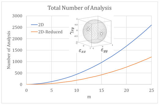
| + | <span style="text-align: center; font-size: 75%;">'''Figure 2.''' Total number of analysis for 2D and 2D Reduced case and 3D Strain Space.</span></div> | ||
| + | |||
| + | Introducing the parameter <math display="inline">\, m\in \, \left[ 1,inf\right[</math> as subdivision of the interval <math display="inline">[0,\pi ]</math> we can uniquely define the strain direction with a pair of integer parameter <math display="inline">\in [-</math><math>m,m]</math>, that we will call ''tag''. With this method, each point was equally spaced from the other and the angles <math display="inline">\theta</math> and <math display="inline">\varphi</math> varying between <math display="inline">[\frac{-\pi }{m},\frac{\pi }{m}]</math>. In that way, we can observe that the total amount of analysis is <math display="inline">{\left( 2\cdot m+1\right) }^{2}</math>. Considering the superposition of the same resulting strain direction the amount of strain histories will be reduced to ( <math display="inline">2\cdot m</math>)( <math display="inline">m-</math><math>1</math>)+2. Despite this reduction, we will remark that using a high value of'' m'' implies an exponential increasing of the analysis, see Figure 2 above. | ||
| + | |||
| + | Once the strain loading directions are computed, we apply them to the RVE doing a classical First Order Multiscale Analysis [8]. During the analysis all the degrees of freedom are fixed and for each <math display="inline">n</math> time step we will solve the microscale problem, evaluating the homogenized stress and constitutive tensor. With this information we can determine the corresponding value of equivalent damage at each time step. | ||
| + | |||
| + | ==='''3.2''' Equivalent damage definition === | ||
| + | |||
| + | During a classical full multiscale analysis, the RVE is solved at each time step even if the linear elastic limit of the material is not achieved. In terms of optimization, it represents wasted time consumption. In this paper, we will introduce a key parameter, called equivalent damage, that provide this limit as the relation between the homogenized stress and the corresponding elastic one. This parameter is defined as: | ||
| + | |||
| + | {| class="formulaSCP" style="width: 100%; text-align: center;" | ||
| + | |- | ||
| + | | | ||
| + | {| style="text-align: center; margin:auto;" | ||
| + | |- | ||
| + | | <math display="inline">{d}_{eq}=\frac{\parallel {\sigma }_{el}-{\sigma }_{real}\parallel }{\parallel {\sigma }_{el}\parallel },{d}_{eq}\in [0,1]</math> | ||
| + | |} | ||
| + | | style="width: 5px;text-align: right;white-space: nowrap;" | (3) | ||
| + | |} | ||
| + | |||
| + | |||
| + | where <math display="inline">{\sigma }_{real}</math> is the homogenized stress, <math display="inline">{\sigma }_{el}=</math><math>{C}_{el}^{H}:\epsilon</math> is the elastic stress and <math display="inline">{C}_{el}^{H}</math> is the Homogenized Constitutive Elastic Tensor. | ||
| + | |||
| + | The discretization of the RVE response with a unique parameter is needed for the interpolation of the DB information. In this way, we can obtain the stress flux surface at certain equivalent damage level and reconstruct the RVE behavior for any strain direction interpolating the stored homogenized stress data. | ||
| + | |||
| + | ==='''3.3''' Discrete Multiscale Threshold Surface=== | ||
| + | |||
| + | Fixing the <math display="inline">{d}_{eq}</math> equal to 0.1, that the author defined as the linear elastic threshold of the microstructure, the Discrete Multiscale Threshold Surface is represented by the corresponding stress at each tag studied. | ||
| + | |||
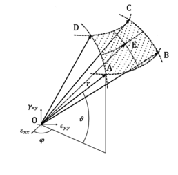
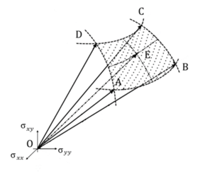
| + | In Figure 3 and 4 we report a 3D visualization of a portion of the DMTS and the algorithm of the proposed method, where the point E represents the intersection of the direction of the stress and strain with the elastic limit surface. The points A, B, C, D correspond to the nearest tag surrounding this direction used to interpolate the results. | ||
| + | |||
| + | ==='''3.4''' Discrete Multiscale Constitutive Model=== | ||
| + | |||
| + | Starting from the model presented above, the second proposed method is an extension of the DMTS. Indeed, DMCM provides a complete definition of RVE behavior storing in a Database the stress-strain response related to the equivalent damage parameter defined previously. | ||
| + | |||
| + | <div class="center" style="width: auto; margin-left: auto; margin-right: auto;"> | ||
| + | |||
| + | {| | ||
| + | |- | ||
| + | | [[Image:Zaghi_et_al_2021a-image7-c.png|258px]] | ||
| + | | [[Image:Zaghi_et_al_2021a-image8.png|center|282px]] | ||
| + | |} | ||
| + | </div> | ||
| + | |||
| + | <div class="center" style="width: auto; margin-left: auto; margin-right: auto;"> | ||
| + | :(a) (b)</div> | ||
| + | |||
| + | <div class="center" style="width: auto; margin-left: auto; margin-right: auto;"> | ||
| + | <span style="text-align: center; font-size: 75%;">'''Figure 3.''' Graphical representation of (a)Strain Space and (b) Stress Space for DMTS.</span></div> | ||
| + | |||
| + | <div class="center" style="width: auto; margin-left: auto; margin-right: auto;"> | ||
| + | [[Image:Zaghi_et_al_2021a-image9.png|366px]] </div> | ||
| + | |||
| + | <div class="center" style="width: auto; margin-left: auto; margin-right: auto;"> | ||
| + | <span style="text-align: center; font-size: 75%;">'''Figure 4.''' DMTS Algorithm.</span></div> | ||
| + | |||
| + | Instead of only one value, corresponding to the elastic limit, for the DMCM multiple threshold surfaces are computed. The non-linear behavior of the RVE will be discretized with a series of equivalent damage levels ranging from 0 to 1. In this way, during the RVE analysis the strain increment is iteratively adapted to reach the correct strain increment (for each strain direction) that gives an iso-Damage surface. After that, FE2 analysis are no longer needed. Indeed, an additional interpolation method over the stored threshold surfaces could be performed to predict the behavior of the macrostructure at each integration point. | ||
| + | |||
| + | The figure below can provide how the proposed algorithm works with a graphical representation. | ||
| + | |||
| + | <div class="center" style="width: auto; margin-left: auto; margin-right: auto;"> | ||
| + | |||
| + | {| | ||
| + | |- | ||
| + | | [[Image:Zaghi_et_al_2021a-image10.png|282px]] | ||
| + | | [[Image:Zaghi_et_al_2021a-image11-c.png|center|288px]] | ||
| + | |} | ||
| + | </div> | ||
| + | |||
| + | <div class="center" style="width: auto; margin-left: auto; margin-right: auto;"> | ||
| + | :(a) (b)</div> | ||
| + | |||
| + | <div class="center" style="width: auto; margin-left: auto; margin-right: auto;"> | ||
| + | <span style="text-align: center; font-size: 75%;">'''Figure 5.''' Graphical representation of (a)Strain Space and (b) Stress Space Evolution for DMCM.</span></div> | ||
| + | |||
| + | The points E and E’ represent the intersection of the direction of the stress and strain with the surfaces at damage ''i'' and ''ii''. The points A,B,C,D and A’,B’,C’,D’ corresponds to the nearest tag that is surrounding this direction for the different level of damage. | ||
| + | |||
| + | The value of strain and stress for the points E and E’ were determined by interpolating the data from the DB of the nearest tag for each level of damage. In that way we can reconstruct the stress strain response of the RVE for any possible direction in the strain space. | ||
| + | |||
| + | The DMCM algorithm could be resumed in the figure 6: | ||
| + | |||
| + | <div class="center" style="width: auto; margin-left: auto; margin-right: auto;"> | ||
| + | [[Image:Zaghi_et_al_2021a-image12.png|390px]] </div> | ||
| + | |||
| + | <div class="center" style="width: auto; margin-left: auto; margin-right: auto;"> | ||
| + | <span style="text-align: center; font-size: 75%;">'''Figure 6.''' DMCM Algorithm.</span></div> | ||
| + | |||
| + | We will remark that, creating the DB with strain-controlled analysis, the reference surfaces in the strain space are concentric; on the other hand, in the stress space this is not obvious and depends on the geometry and the constitutive laws involved in the RVE. | ||
| + | |||
| + | <span id='_3znysh7'></span>The DB scheme provides at first level the tag. Then, for each tag, we will store the information of <math display="inline">\sigma</math> and <math display="inline">\lambda</math> (lambda) at different values of equivalent damage. | ||
| + | |||
| + | <div class="center" style="width: auto; margin-left: auto; margin-right: auto;"> | ||
| + | [[Image:Zaghi_et_al_2021a-image13.png|528px]] </div> | ||
| + | |||
| + | <div class="center" style="width: auto; margin-left: auto; margin-right: auto;"> | ||
| + | <span style="text-align: center; font-size: 75%;">'''Figure 7.''' DMCM algorithm.</span></div> | ||
| + | |||
| + | Considering the number of analyses needed for the creation of the stress-strain DB, which is proportional to the discretization parameter m, it is obvious that as long as the number of RVEs needed by the macroscale structure is higher than the number of Strain Histories, the advantages of the proposed method increases. | ||
| + | |||
| + | ==4 Reinforced composite stiffener section== | ||
| + | |||
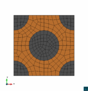
| + | In this section we analyze a reinforced composite beam comparing the three proposed methods: FE2, DMTS and DMCM. The microscale used is a long fiber reinforced composite, composed by F155 Epoxy Resin matrix and Carbon fiber (simulated as elastic material for simplicity). The geometry of the RVE was composed by 5 symmetric inclusions as it is shown in Figure 8 and the mesh used for the micro scale is composed by 272 small displacement linear elements with 305 nodes. The analysis was performed by using plane stress theory and considering 200mm as thickness for the stiffener. | ||
| + | |||
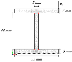
| + | The geometry and boundary conditions of the beam are also described in Figure 8. The macroscale structure is composed by 1075 triangular elements and 678 nodes subjected to a vertical displacement <math display="inline">{u}_{y}</math>. In order to simplify the analysis, in case of Full Multiscale and DMTS methods, only 84 elements are considered with double scale, using elastic homogenized properties in the rest of the structure. | ||
| + | |||
| + | <div class="center" style="width: auto; margin-left: auto; margin-right: auto;"> | ||
| + | |||
| + | {| | ||
| + | |- | ||
| + | | [[Image:Zaghi_et_al_2021a-image14-c.png|294px]] | ||
| + | | [[Image:Zaghi_et_al_2021a-image15.png|center|174px]] | ||
| + | |} | ||
| + | </div> | ||
| + | |||
| + | <div class="center" style="width: auto; margin-left: auto; margin-right: auto;"> | ||
| + | <span style="text-align: center; font-size: 75%;">'''Figure 8.''' Reinforced composite stiffener section and RVE geometry and mesh.</span></div> | ||
| + | |||
| + | <div class="center" style="width: auto; margin-left: auto; margin-right: auto;"> | ||
| + | <span style="text-align: center; font-size: 75%;">'''Table 1.''' Mechanical properties of composite RVE</span></div> | ||
| + | {| style="width: 100%;margin: 1em auto 0.1em auto;border-collapse: collapse;" | ||
| + | |- | ||
| + | | colspan='3' style="text-align: center;"|<span style="text-align: center; font-size: 75%;">'''F155 Epoxy Resin Mechanical Properties'''</span> | ||
| + | |- | ||
| + | | style="border: 1pt solid black;text-align: center;"|<span style="text-align: center; font-size: 75%;">Young Modulus</span> | ||
| + | | style="border: 1pt solid black;text-align: center;"|<span style="text-align: center; font-size: 75%;">3.24e3</span> | ||
| + | | colspan='2' style="border: 1pt solid black;text-align: center;vertical-align: top;"|<span style="text-align: center; font-size: 75%;">MPa</span> | ||
| + | |- | ||
| + | | style="border: 1pt solid black;text-align: center;"|<span style="text-align: center; font-size: 75%;">Poisson Ratio</span> | ||
| + | | style="border: 1pt solid black;text-align: center;"|<span style="text-align: center; font-size: 75%;">0.32</span> | ||
| + | | colspan='2' style="border: 1pt solid black;text-align: center;vertical-align: top;"| | ||
| + | |- | ||
| + | | style="border: 1pt solid black;text-align: center;"|<span style="text-align: center; font-size: 75%;">Stress Traction Limit</span> | ||
| + | | style="border: 1pt solid black;text-align: center;"|<span style="text-align: center; font-size: 75%;">80</span> | ||
| + | | colspan='2' style="border: 1pt solid black;text-align: center;vertical-align: top;"|<span style="text-align: center; font-size: 75%;">MPa</span> | ||
| + | |- | ||
| + | | style="border: 1pt solid black;text-align: center;"|<span style="text-align: center; font-size: 75%;">Traction Fracture Energy</span> | ||
| + | | style="border: 1pt solid black;text-align: center;"|<span style="text-align: center; font-size: 75%;">0.73</span> | ||
| + | | colspan='2' style="border: 1pt solid black;text-align: center;vertical-align: top;"|<span style="text-align: center; font-size: 75%;">J/mm2</span> | ||
| + | |- | ||
| + | | style="border: 1pt solid black;text-align: center;"|<span style="text-align: center; font-size: 75%;">Stress Compression Limit</span> | ||
| + | | style="border: 1pt solid black;text-align: center;"|<span style="text-align: center; font-size: 75%;">240</span> | ||
| + | | colspan='2' style="border: 1pt solid black;text-align: center;vertical-align: top;"|<span style="text-align: center; font-size: 75%;">MPa</span> | ||
| + | |- | ||
| + | | style="border: 1pt solid black;text-align: center;"|<span style="text-align: center; font-size: 75%;">Compression Fracture Energy</span> | ||
| + | | style="border: 1pt solid black;text-align: center;"|<span style="text-align: center; font-size: 75%;">2.19</span> | ||
| + | | colspan='2' style="border: 1pt solid black;text-align: center;vertical-align: top;"|<span style="text-align: center; font-size: 75%;">J/mm2</span> | ||
| + | |- | ||
| + | | colspan='3' style="text-align: center;"|<span style="text-align: center; font-size: 75%;">'''Carbon Fiber Mechanical Properties'''</span> | ||
| + | |- | ||
| + | | style="border: 1pt solid black;text-align: center;"|<span style="text-align: center; font-size: 75%;">Young Modulus</span> | ||
| + | | style="border: 1pt solid black;text-align: center;"|<span style="text-align: center; font-size: 75%;">235e3</span> | ||
| + | | colspan='2' style="border: 1pt solid black;text-align: center;vertical-align: top;"|<span style="text-align: center; font-size: 75%;">MPa</span> | ||
| + | |- | ||
| + | | style="border: 1pt solid black;text-align: center;"|<span style="text-align: center; font-size: 75%;">Poisson Ratio</span> | ||
| + | | style="border: 1pt solid black;text-align: center;"|<span style="text-align: center; font-size: 75%;">0.21</span> | ||
| + | | colspan='2' style="border: 1pt solid black;text-align: center;vertical-align: top;"| | ||
| + | |} | ||
| + | |||
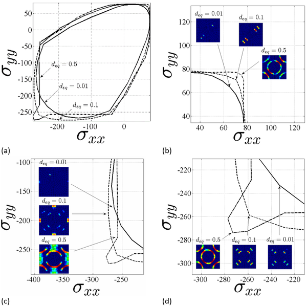
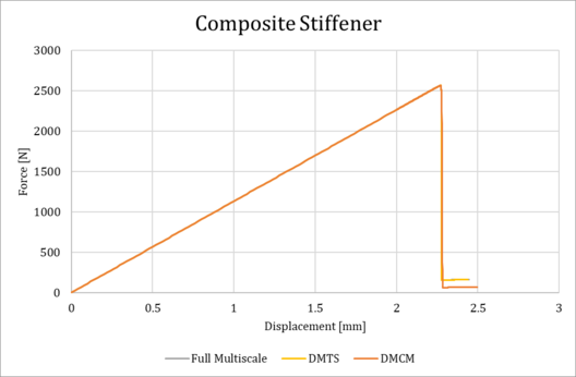
| + | Below (Figure 9) are reported the sections of the elastic limit surface for d=0.01 and the stress evolution for d=0.1,0.5 for the composite. Figure 10 shows the force-displacement curves of DMTS and DMCM methods. As it can be seen, they overlap and achieve the same maximum value of force of the FM2 case. | ||
| + | |||
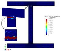
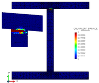
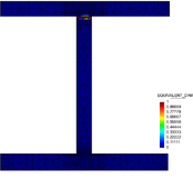
| + | Finally, in Figure 11 is shown the equivalent damage distribution on the stiffener and in the microstructure for the different models developed. | ||
| + | |||
| + | <div class="center" style="width: auto; margin-left: auto; margin-right: auto;"> | ||
| + | [[Image:Zaghi_et_al_2021a-image16.png|600px]] </div> | ||
| + | |||
| + | <div class="center" style="width: auto; margin-left: auto; margin-right: auto;"> | ||
| + | <span style="text-align: center; font-size: 75%;">'''Figure 9.''' RVE Stress Evolution Surfaces.</span></div> | ||
| + | |||
| + | <div class="center" style="width: auto; margin-left: auto; margin-right: auto;"> | ||
| + | [[Image:Zaghi_et_al_2021a-image17.png|528px]] </div> | ||
| + | |||
| + | <div class="center" style="width: auto; margin-left: auto; margin-right: auto;"> | ||
| + | <span style="text-align: center; font-size: 75%;">'''Figure 10.''' Comparison Force-Displacement curves.</span></div> | ||
| + | |||
| + | <div class="center" style="width: auto; margin-left: auto; margin-right: auto;"> | ||
| + | |||
| + | {| | ||
| + | |- | ||
| + | | [[Image:Zaghi_et_al_2021a-image18-c.png|198px]] | ||
| + | | [[Image:Zaghi_et_al_2021a-image19-c.png|center|204px]] | ||
| + | |} | ||
| + | [[Image:Zaghi_et_al_2021a-image20-c.png|174px]] </div> | ||
| + | |||
| + | <div class="center" style="width: auto; margin-left: auto; margin-right: auto;"> | ||
| + | (a) (b) (c)</div> | ||
| + | |||
| + | <div class="center" style="width: auto; margin-left: auto; margin-right: auto;"> | ||
| + | <span style="text-align: center; font-size: 75%;">'''Figure 11.''' Equivalent damage distribution for (a) FE2, (b) DMTS, (c) DMCM.</span></div> | ||
| + | |||
| + | In case of reinforce composite stiffener, computational effort decreases significantly using the optimization method proposed in this paper. Indeed, as we can see in Table 2, we obtain a speed-up of 4.7 and 661.2 for DMTS and DMCM method respectively. Despite of the 70 RVEs generated in the DMTS, against the 84 of the FE2, we are still having advantages using this method. | ||
| + | |||
| + | <div class="center" style="width: auto; margin-left: auto; margin-right: auto;"> | ||
| + | <span style="text-align: center; font-size: 75%;">'''Table 2.''' Comparison of time and computational cost</span></div> | ||
| + | {| style="width: 100%;border-collapse: collapse;" | ||
| + | |- | ||
| + | | style="border: 1pt solid black;text-align: center;vertical-align: top;"|<span style="text-align: center; font-size: 75%;">'''Type'''</span> | ||
| + | | style="border: 1pt solid black;text-align: center;vertical-align: top;"|<span style="text-align: center; font-size: 75%;">'''Time [s]'''</span> | ||
| + | | style="border: 1pt solid black;text-align: center;vertical-align: top;"|<span style="text-align: center; font-size: 75%;">'''Memory [MB]'''</span> | ||
| + | | style="border: 1pt solid black;text-align: center;vertical-align: top;"|<span style="text-align: center; font-size: 75%;">'''Active RVEs'''</span> | ||
| + | | style="border: 1pt solid black;text-align: center;vertical-align: top;"|<span style="text-align: center; font-size: 75%;">'''Time Speedup'''</span> | ||
| + | |- | ||
| + | | style="border: 1pt solid black;vertical-align: top;"|<span style="text-align: center; font-size: 75%;">FE2</span> | ||
| + | | style="border: 1pt solid black;text-align: center;vertical-align: top;"|<span style="text-align: center; font-size: 75%;">40,267.5</span> | ||
| + | | style="border: 1pt solid black;text-align: center;vertical-align: top;"|<span style="text-align: center; font-size: 75%;">152.2</span> | ||
| + | | style="border: 1pt solid black;text-align: center;vertical-align: top;"|<span style="text-align: center; font-size: 75%;">84/1075</span> | ||
| + | | style="border: 1pt solid black;text-align: center;vertical-align: top;"|<span style="text-align: center; font-size: 75%;">-</span> | ||
| + | |- | ||
| + | | style="border: 1pt solid black;vertical-align: top;"|<span style="text-align: center; font-size: 75%;">DMTS</span> | ||
| + | | style="border: 1pt solid black;text-align: center;vertical-align: top;"|<span style="text-align: center; font-size: 75%;">8,609.9</span> | ||
| + | | style="border: 1pt solid black;text-align: center;vertical-align: top;"|<span style="text-align: center; font-size: 75%;">108.7</span> | ||
| + | | style="border: 1pt solid black;text-align: center;vertical-align: top;"|<span style="text-align: center; font-size: 75%;">70/1075</span> | ||
| + | | style="border: 1pt solid black;text-align: center;vertical-align: top;"|<span style="text-align: center; font-size: 75%;">4.7</span> | ||
| + | |- | ||
| + | | style="border: 1pt solid black;vertical-align: top;"|<span style="text-align: center; font-size: 75%;">DMCM</span> | ||
| + | | style="border: 1pt solid black;text-align: center;vertical-align: top;"|<span style="text-align: center; font-size: 75%;">60.9</span> | ||
| + | | style="border: 1pt solid black;text-align: center;vertical-align: top;"|<span style="text-align: center; font-size: 75%;">33.1</span> | ||
| + | | style="border: 1pt solid black;text-align: center;vertical-align: top;"|<span style="text-align: center; font-size: 75%;">0/1075</span> | ||
| + | | style="border: 1pt solid black;text-align: center;vertical-align: top;"|<span style="text-align: center; font-size: 75%;">661.2</span> | ||
| + | |} | ||
| + | |||
| + | Moreover, DMCM it is clearly faster than FM2 and DMTS as well. The linear interpolation of the RVE strain history can provide a non-linear behavior of the macrostructure, able to reproduce crack initiation and propagation. | ||
| + | |||
| + | ==5 Conclusions== | ||
| + | |||
| + | First order multiscale homogenization method can fully describe both linear and non-linear behavior of complex microstructures and the impact they have on the macroscale response. However, the computational cost required to analyze large structures is not negligible. In the last years, many optimization methods have been developed to overcome this problem. In this paper, the authors propose two optimization techniques that can provide a significant speed-up compared to the classical FE2 without loss of accuracy on the final results. From the RVE FE analysis, the Discrete Multiscale Threshold Surface gives the linear elastic limit to determine where the 2-scale computations are required at the structural level, while the DMCM can conduct the analysis without solving the micro-scale model, since it can describe both linear and nonlinear regimes. The keys of both methods are the precomputed Stress-Strain DataBase and the equivalent damage parameter, essential to reconstruct the correct behavior of the structure. | ||
| + | |||
| + | DMTS and DMCM methods are validated by a reinforced composite stiffener, showing the capability and robustness of these techniques. The achieved speed-up of more than 600 times respect to FE2 and the accuracy of the results, justifies the time spent to obtain the Stress-Strain DataBase. | ||
| + | |||
| + | ==References == | ||
| + | |||
| + | <span style="text-align: center; font-size: 75%;">[1]</span> <span style="text-align: center; font-size: 75%;">H.J. Böhm, ''Mechanics of Microstructured Materials'', '''464''', pág. 1-40 (2004).</span> | ||
| + | |||
| + | [https://doi.org/10.1007/978-3-7091-2776-6_1 https://doi.org/10.1007/978-3-7091-2776-6_1] | ||
| + | |||
| + | <span style="text-align: center; font-size: 75%;">[2]</span> <span style="text-align: center; font-size: 75%;">F.Otero, X.Martinez, S.Oller, O.Salomon, ''Compos Struct'', '''131''', 11, pág. 707-719 (2015).</span> | ||
| + | |||
| + | [https://doi.org/10.1016/j.compstruct.2015.06.006 https://doi.org/10.1016/j.compstruct.2015.06.006] | ||
| + | |||
| + | <span style="text-align: center; font-size: 75%;">[3]</span> <span style="text-align: center; font-size: 75%;">M..Petracca et al., ''Comp Mect'', '''57''', 2, pág. 256-276 (2016).</span> | ||
| + | |||
| + | [https://doi.org/10.1007/s00466-015-1230-6 https://doi.org/10.1007/s00466-015-1230-6] | ||
| + | |||
| + | <span style="text-align: center; font-size: 75%;">[4]</span> <span style="text-align: center; font-size: 75%;">P.M.Suquet, ''Plasticity Today'', '''5''', pág. 279-309 (1985).</span> | ||
| + | |||
| + | URL: [https://ci.nii.ac.jp/naid/10009833388/en/ https://ci.nii.ac.jp/naid/10009833388/en/] | ||
| + | |||
| + | <span style="text-align: center; font-size: 75%;">[5]</span> <span style="text-align: center; font-size: 75%;">M.Geers et al., ''Int J Multiscale Comput Eng'', '''1''', 4, pág. 371-386 (2003).</span> | ||
| + | |||
| + | [https://doi.org/10.1016/j.cam.2009.08.077 https://doi.org/10.1016/j.cam.2009.08.077] | ||
| + | |||
| + | <span style="text-align: center; font-size: 75%;">[6]</span> <span style="text-align: center; font-size: 75%;">T.Kanit et al., ''Int J Solids Struct'', '''40''', 13, pág. 3647-3679 (2003). [https://doi.org/10.1016/S0020-7683(03)00143-4 https://doi.org/10.1016/S0020-7683(03)00143-4] </span> | ||
| + | |||
| + | <span style="text-align: center; font-size: 75%;">[7]</span> <span style="text-align: center; font-size: 75%;">J.</span> <span style="text-align: center; font-size: 75%;">Hernández, et al., ''Comput Methods Appl Mech Eng'', '''276''', pág. 149-189 (2014).</span> | ||
| + | |||
| + | [https://doi.org/10.1016/j.cma.2014.03.011 https://doi.org/10.1016/j.cma.2014.03.011] | ||
| + | |||
| + | <span style="text-align: center; font-size: 75%;">[8]</span> <span style="text-align: center; font-size: 75%;">F.Otero, S.Oller, X.Martinez, ''Arch Comp Meth Eng'', '''25''', pág. 479-505 (2018).</span> | ||
| + | |||
| + | [https://doi.org/10.1007/s11831-016-9205-0 https://doi.org/10.1007/s11831-016-9205-0] | ||
Latest revision as of 20:54, 12 December 2022
1 Introduction
Nowadays, numerous materials used in engineering industrial field, as well as in biological and biomedical area, are characterized by two or more constituents, also called phases.
Carbon fiber composites, polycrystalline structures, concrete, bone or wood are only some examples of components where the constituents could be distinguished at certain length scale. These materials are called inhomogeneous. The length scale as well as the type of constituents are only some example of possible criterion to classify them. Indeed, microstructure take an important role during the analysis of the material because of the topology and the properties of each phase that determines its behavior.
It is also possible to say that defining a microscale structure means to study the behavior of each phase in order to determine the overall behavior of the global structure in terms of physical properties such as mechanical, thermal, electrical, etc.
Geometry, structure, properties and behavior of the inhomogeneous materials could be separated in two different fields depending on its length scale. On one hand, the microscale (or fine-scale) corresponds to the microstructure where each phase is distinguishable. On the other hand, the macroscale (or coarse-scale) is the largest scale (and length) of the model, in contrast to the microscale that represents the lowest scale.
The most important assumption that has to be made when studying the micromechanical models is the scale separation between micro and macro structures. That assumption allows to separate the contribution of the microscale, defined as fluctuation part, from the macroscale ones, the constant part.
As it is explained in Bohm [1] these two contributions can be distinguished as fast and slow variables, where the fast variables, microscale fluctuations, can influence the behavior of the macroscale only through their volume average. Instead, the slow variables, the macroscale contribution, are not significant at the microscale level and can be considered as locally constant.
Otero et al. [2] and Petracca et al. [3], also provides an efficient multiscale strategy that, in case of first-order homogenization (FE2), ensures the macro and micro mesh independence taking into account the conservation of the energy dissipation of through the scales.
2 Multiscale Methods
One of the most popular multiscale methods is the first-order homogenization. In this procedure, the strain obtained when analyzing the macroscopic structure is used to define the boundary conditions, applied on a Representative Volume Element RVE, to solve the Boundary Value Problem (BVP) at the microscale.
The basic principles of homogenization method were provided by Suquet [4] to obtain the constitutive equation for the homogenized properties of a heterogeneous material. The unit cell is defined as a microscopic subregion that is representative of the entire microstructure in an average sense. The RVE is employed to obtain the effective properties for the homogenized material because it is assumed that it must contain a sufficient number of heterogeneities [5] [6].
The solution of the problem at the microscale, under such conditions, acts as an equivalent constitutive law for the macroscale, and it provides material stiffness and stresses as the volume average of the microscopic ones. This equivalent constitutive law is used in all the integration points of the macroscopic model to obtain the global response of the structure. When dealing with nonlinear microstructures, it will lead to an iterative procedure in which the RVE must be solved for different boundary conditions until both scales reach equilibrium, ensuring consistency between the micro- and macroscale solutions.
The first-order homogenization technique developed assumes a scale separation between the macro and the microscale, that is, the characteristic length of the microscale should be much smaller than the length of the macroscale elements, L: l<<L [7].
The main steps of the classical FE2 technique can be resumed in the figure below. On each integration point of the discretized macroscale domain, the macroscopic strain tensor provides the input variables for the microscale domain. Then, the solution of the microscopic behavior of the RVE provides the macroscopic output and properties of the equivalent homogeneous medium.
In this paper, for the sake of simplicity, the procedure assumes small displacements and a quasi-static behavior in both macro and micro scales. However, the methodology proposed can be extended to other cases.
3 Discrete Multiscale Threshold Surface (DMTS) and Discrete Multiscale Constitutive Model (DMCM)
The purpose of this paper is to provide two multiscale optimization techniques, directly derived from the classical first order multiscale theory. Considering these two methods, the main hypothesis is to construct a stress-strain state collector based on multiple RVE simulations able to describe the microscale behavior. Using an Equivalent Damage Parameter ( ), index of the difference between the real and the elastic stress, the Discrete Multiscale Threshold Surface (DMTS) will identify with a finite number of points within the strain space the initiation of the non-linearity of the RVE. The DMTS is intended to reduce the computational cost of FE2, by identifying, during the analysis, where the RVE generation is needed and where the homogenized elastic properties are sufficient to obtain the macroscale response. As an extension of the DMTS, the Discrete Multiscale Constitutive Model (DMCM) aims to describe the complete behavior of the microstructure identifying multiple threshold surfaces related to increasing levels of decoupling the analysis from the FE2 methods.
Below, the authors will describe in detail all the aspects of both methods, providing examples and algorithms used for the numerical implementation.
3.1 Strain database definition
In general, due to the complexity of the RVE, we cannot know a-priori the real stress behavior of the microscale. To overcome this problem, we will study the strain space doing a preliminary analysis of the RVE for different loading cases storing the stress response of the structure. These strains, defined as strain histories, are in the multidimensional spaces for 2D or for 3D mechanical problems.
To make accessible this information during the analysis we will store the strain histories in a Homogenized Strain Database. In this chapter, for simplicity, we will only describe the 2D case, but it is perfectly extendable to 3D.
To obtain a complete definition of the microscale behavior we will impose as strain histories the value of evenly spaced point projected on the sphere of unitary radius centered in the origin of the axes . We can uniquely define these points in 3D spherical coordinates system as the combination of three parameters ( ), as we can see in the Figure 2, where the angles and represents the direction of the strain loads that we applied to the microscale and is the unitary strain intensity.
Then we can obtain the components of the strain vector in cartesian coordinates as:
|
|
(1) |
|
|
(2) |
From Eq. 1 we can observe that the strain is periodic with sin and cos functions of and and these two angles can be varying between . The subdivision of this interval determines the number of analyses to preform and the precision of the discretization.
Introducing the parameter as subdivision of the interval we can uniquely define the strain direction with a pair of integer parameter , that we will call tag. With this method, each point was equally spaced from the other and the angles and varying between . In that way, we can observe that the total amount of analysis is . Considering the superposition of the same resulting strain direction the amount of strain histories will be reduced to ( )( )+2. Despite this reduction, we will remark that using a high value of m implies an exponential increasing of the analysis, see Figure 2 above.
Once the strain loading directions are computed, we apply them to the RVE doing a classical First Order Multiscale Analysis [8]. During the analysis all the degrees of freedom are fixed and for each time step we will solve the microscale problem, evaluating the homogenized stress and constitutive tensor. With this information we can determine the corresponding value of equivalent damage at each time step.
3.2 Equivalent damage definition
During a classical full multiscale analysis, the RVE is solved at each time step even if the linear elastic limit of the material is not achieved. In terms of optimization, it represents wasted time consumption. In this paper, we will introduce a key parameter, called equivalent damage, that provide this limit as the relation between the homogenized stress and the corresponding elastic one. This parameter is defined as:
|
|
(3) |
where is the homogenized stress, is the elastic stress and is the Homogenized Constitutive Elastic Tensor.
The discretization of the RVE response with a unique parameter is needed for the interpolation of the DB information. In this way, we can obtain the stress flux surface at certain equivalent damage level and reconstruct the RVE behavior for any strain direction interpolating the stored homogenized stress data.
3.3 Discrete Multiscale Threshold Surface
Fixing the equal to 0.1, that the author defined as the linear elastic threshold of the microstructure, the Discrete Multiscale Threshold Surface is represented by the corresponding stress at each tag studied.
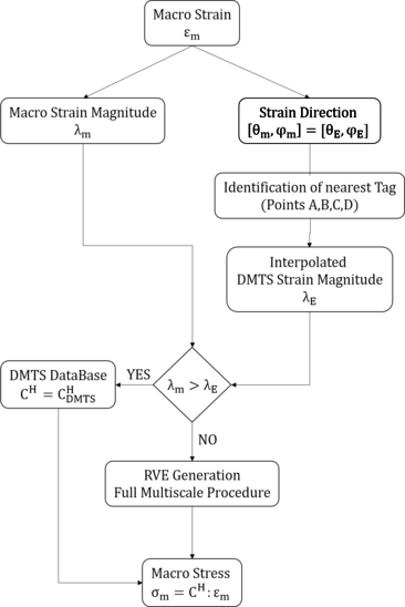
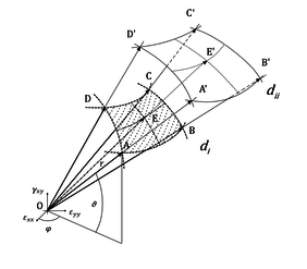
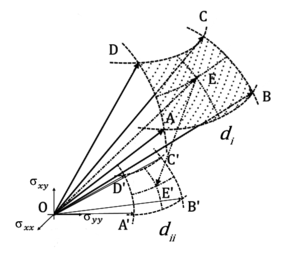
In Figure 3 and 4 we report a 3D visualization of a portion of the DMTS and the algorithm of the proposed method, where the point E represents the intersection of the direction of the stress and strain with the elastic limit surface. The points A, B, C, D correspond to the nearest tag surrounding this direction used to interpolate the results.
3.4 Discrete Multiscale Constitutive Model
Starting from the model presented above, the second proposed method is an extension of the DMTS. Indeed, DMCM provides a complete definition of RVE behavior storing in a Database the stress-strain response related to the equivalent damage parameter defined previously.
- (a) (b)
Instead of only one value, corresponding to the elastic limit, for the DMCM multiple threshold surfaces are computed. The non-linear behavior of the RVE will be discretized with a series of equivalent damage levels ranging from 0 to 1. In this way, during the RVE analysis the strain increment is iteratively adapted to reach the correct strain increment (for each strain direction) that gives an iso-Damage surface. After that, FE2 analysis are no longer needed. Indeed, an additional interpolation method over the stored threshold surfaces could be performed to predict the behavior of the macrostructure at each integration point.
The figure below can provide how the proposed algorithm works with a graphical representation.
- (a) (b)
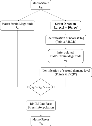
The points E and E’ represent the intersection of the direction of the stress and strain with the surfaces at damage i and ii. The points A,B,C,D and A’,B’,C’,D’ corresponds to the nearest tag that is surrounding this direction for the different level of damage.
The value of strain and stress for the points E and E’ were determined by interpolating the data from the DB of the nearest tag for each level of damage. In that way we can reconstruct the stress strain response of the RVE for any possible direction in the strain space.
The DMCM algorithm could be resumed in the figure 6:
We will remark that, creating the DB with strain-controlled analysis, the reference surfaces in the strain space are concentric; on the other hand, in the stress space this is not obvious and depends on the geometry and the constitutive laws involved in the RVE.
The DB scheme provides at first level the tag. Then, for each tag, we will store the information of and (lambda) at different values of equivalent damage.
Considering the number of analyses needed for the creation of the stress-strain DB, which is proportional to the discretization parameter m, it is obvious that as long as the number of RVEs needed by the macroscale structure is higher than the number of Strain Histories, the advantages of the proposed method increases.
4 Reinforced composite stiffener section
In this section we analyze a reinforced composite beam comparing the three proposed methods: FE2, DMTS and DMCM. The microscale used is a long fiber reinforced composite, composed by F155 Epoxy Resin matrix and Carbon fiber (simulated as elastic material for simplicity). The geometry of the RVE was composed by 5 symmetric inclusions as it is shown in Figure 8 and the mesh used for the micro scale is composed by 272 small displacement linear elements with 305 nodes. The analysis was performed by using plane stress theory and considering 200mm as thickness for the stiffener.
The geometry and boundary conditions of the beam are also described in Figure 8. The macroscale structure is composed by 1075 triangular elements and 678 nodes subjected to a vertical displacement . In order to simplify the analysis, in case of Full Multiscale and DMTS methods, only 84 elements are considered with double scale, using elastic homogenized properties in the rest of the structure.
| F155 Epoxy Resin Mechanical Properties | |||
| Young Modulus | 3.24e3 | MPa | |
| Poisson Ratio | 0.32 | ||
| Stress Traction Limit | 80 | MPa | |
| Traction Fracture Energy | 0.73 | J/mm2 | |
| Stress Compression Limit | 240 | MPa | |
| Compression Fracture Energy | 2.19 | J/mm2 | |
| Carbon Fiber Mechanical Properties | |||
| Young Modulus | 235e3 | MPa | |
| Poisson Ratio | 0.21 | ||
Below (Figure 9) are reported the sections of the elastic limit surface for d=0.01 and the stress evolution for d=0.1,0.5 for the composite. Figure 10 shows the force-displacement curves of DMTS and DMCM methods. As it can be seen, they overlap and achieve the same maximum value of force of the FM2 case.
Finally, in Figure 11 is shown the equivalent damage distribution on the stiffener and in the microstructure for the different models developed.
In case of reinforce composite stiffener, computational effort decreases significantly using the optimization method proposed in this paper. Indeed, as we can see in Table 2, we obtain a speed-up of 4.7 and 661.2 for DMTS and DMCM method respectively. Despite of the 70 RVEs generated in the DMTS, against the 84 of the FE2, we are still having advantages using this method.
| Type | Time [s] | Memory [MB] | Active RVEs | Time Speedup |
| FE2 | 40,267.5 | 152.2 | 84/1075 | - |
| DMTS | 8,609.9 | 108.7 | 70/1075 | 4.7 |
| DMCM | 60.9 | 33.1 | 0/1075 | 661.2 |
Moreover, DMCM it is clearly faster than FM2 and DMTS as well. The linear interpolation of the RVE strain history can provide a non-linear behavior of the macrostructure, able to reproduce crack initiation and propagation.
5 Conclusions
First order multiscale homogenization method can fully describe both linear and non-linear behavior of complex microstructures and the impact they have on the macroscale response. However, the computational cost required to analyze large structures is not negligible. In the last years, many optimization methods have been developed to overcome this problem. In this paper, the authors propose two optimization techniques that can provide a significant speed-up compared to the classical FE2 without loss of accuracy on the final results. From the RVE FE analysis, the Discrete Multiscale Threshold Surface gives the linear elastic limit to determine where the 2-scale computations are required at the structural level, while the DMCM can conduct the analysis without solving the micro-scale model, since it can describe both linear and nonlinear regimes. The keys of both methods are the precomputed Stress-Strain DataBase and the equivalent damage parameter, essential to reconstruct the correct behavior of the structure.
DMTS and DMCM methods are validated by a reinforced composite stiffener, showing the capability and robustness of these techniques. The achieved speed-up of more than 600 times respect to FE2 and the accuracy of the results, justifies the time spent to obtain the Stress-Strain DataBase.
References
[1] H.J. Böhm, Mechanics of Microstructured Materials, 464, pág. 1-40 (2004).
https://doi.org/10.1007/978-3-7091-2776-6_1
[2] F.Otero, X.Martinez, S.Oller, O.Salomon, Compos Struct, 131, 11, pág. 707-719 (2015).
https://doi.org/10.1016/j.compstruct.2015.06.006
[3] M..Petracca et al., Comp Mect, 57, 2, pág. 256-276 (2016).
https://doi.org/10.1007/s00466-015-1230-6
[4] P.M.Suquet, Plasticity Today, 5, pág. 279-309 (1985).
URL: https://ci.nii.ac.jp/naid/10009833388/en/
[5] M.Geers et al., Int J Multiscale Comput Eng, 1, 4, pág. 371-386 (2003).
https://doi.org/10.1016/j.cam.2009.08.077
[6] T.Kanit et al., Int J Solids Struct, 40, 13, pág. 3647-3679 (2003). https://doi.org/10.1016/S0020-7683(03)00143-4
[7] J. Hernández, et al., Comput Methods Appl Mech Eng, 276, pág. 149-189 (2014).
https://doi.org/10.1016/j.cma.2014.03.011
[8] F.Otero, S.Oller, X.Martinez, Arch Comp Meth Eng, 25, pág. 479-505 (2018).
Document information
Published on 13/10/21
Accepted on 06/10/21
Submitted on 21/09/21
Volume 05 - Comunicaciones Matcomp19 (2021), Issue Núm. 4 - Tesis doctorales presentadas al premio AEMAC a la mejor tesis., 2021
DOI: 10.23967/r.matcomp.2021.10.007
Licence: Other
Share this document
Keywords
claim authorship
Are you one of the authors of this document?
