A Generalized Finite Difference-Volume Hybrid Method Applied to Shallow-Water Equations

Latest revision as of 07:58, 21 July 2022

Abstract

Due to the importance of the shallow-water equations in models of real-life phenomena, in recent years the study and model of problems that involve them have been the object of interest of many people. By reason of this, it is imperative to have efficient numerical methods to obtain an approximation of the solutions of the shallow-water equations.

Several authors have worked in approximations using the well-known finite volume and finite element methods, nevertheless, even when these methods compute good approximations to real-life behavior, the computational cost is usually high, which could be a limitation to the application of these methods.

This paper presents an explicit Generalized Finite Difference-Volume Hybrid approximation to the solution of the shallow-water equations, solved on irregular regions meshed with logically rectangular grids; the numerical results show the accuracy obtained with a low-cost implementation. The proposed scheme is a hybridization of a generalized finite difference scheme with the finite volume method.

keywords hybrid method, finite difference, finite volume, shallow-water equations, irregular regions

1 Introduction

In nature, there exist many types of flow that can be characterized as shallow-water flows. The main characteristic of these kinds of flows is that the vertical scales are much smaller than the horizontal ones. This happens in many regions all over the world, such as lakes, some rivers and, in some special cases, in parts of the oceans.

Since the flow in these cases is almost horizontal, a great number of simplifications can be done in the physical and mathematical formulation taking into account that the value of the pressure is essentially the hydrostatic one. It is important to remark that, even with these simplifications, the formulations are not two-dimensional, since the bottom friction must be taken into account in the boundary layers. In the literature, these ${\textstyle 3D}$ effects are often not essential for the models, and it is only necessary to consider the two-dimensional depth-averaged form [1].

Due to the simplicity of the finite difference methods, some important advances have been done in the approximation to the solution of these equations; Po-Wei and Chia-Ming present in [2] a generalized finite difference method that can produce very good results, with the limitation that the average flow direction has to be known a priori in order to use the generalized finite difference method.

Young discusses a meshless method in [3,4] that can produce very good results in very irregular domains by using a local radial-basis-functions differential-quadrature approach; the results presented in his papers have very good quality and can be applied to real-life scenarios. One more time, even when this method produces very good results, even for inflow problems, the computational cost can be very high.

One of the most common problems that are presented in many works is the treatment of discontinuities and singularities; it is well known that one way to overcome these problems is using a conservative form of the equations. Nevertheless, Ulrik Skre Fjordhol [5], Bruno Gabutti [6], and Carlos Parés [7] have proposed accurate numerical schemes to approximate the solution of non-conservative Hyperbolic Equations, discussing upwind like and splitting schemes for solving numerically this version of the equations. Following the previous ideas, in this paper we present numerical schemes for the conservative form and non-conservative form of the shallow-water equations; the main aim of this work is to obtain an explicit method that can be applied to irregular domains.

In order to do that, let us first consider the problem of obtaining an approximation to the solution of the conservative form of the shallow-water equations

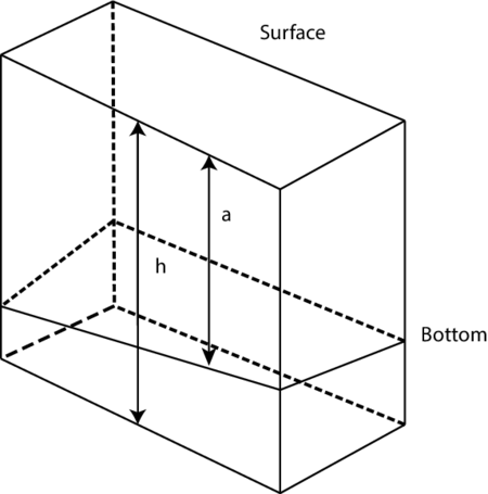
in a simply connected planar domain ${\textstyle \Omega }$ defined by a polygonal boundary, where ${\textstyle h}$ is the water level, ${\textstyle u}$ and ${\textstyle v}$ are the velocity fields in the ${\textstyle x}$ and ${\textstyle y}$ directions respectively, ${\textstyle a}$ is the water-body depth, ${\textstyle f}$ is the Coriolis force and ${\textstyle c_{f}}$ represents the external forces (see figure (1)).

Figure 1: Definition of bottom and free surface.

In these equations, the change of variables

leads to the expressions

(1)

(2)

(3)

here, the unknowns are the conservative quantities ${\textstyle q}$ , ${\textstyle r}$ and ${\textstyle s}$ , that represent the mass and momentum of the physical problem.

After differentiation and some algebra, equations (1) - (3) can be rewritten as

(4)

(5)

(6)

This is the non-conservative form or differential form of the shallow-water equations.

2 Proposed hybrid schemes

The proposed schemes arise from the integral form of equations (2) and (3), (5) and (6), and a finite difference approximation of equations (1) and (4).

2.1 Hybrid schemes on rectangular regions

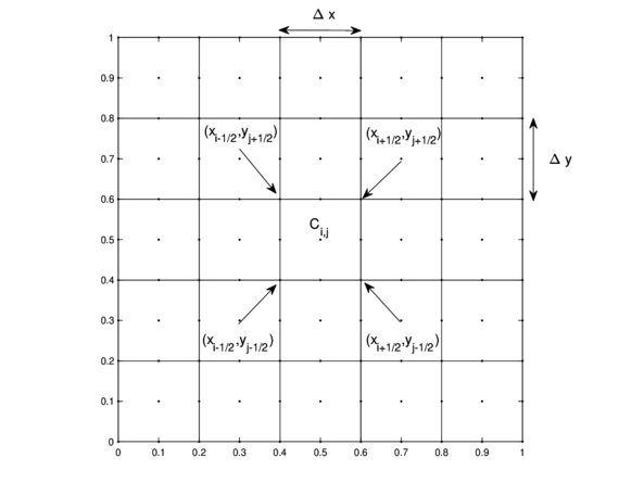
On rectangular regions, the space region can be discretized by taking a grid formed by uniform cells ${\textstyle C_{(i,j)}}$ defined as

as shown on figure (2).

Figure 2: Rectangular meshed region $\Omega$ .

2.1.1 Hybrid scheme for the conservative form

With this discretization of the region, the proposed scheme approximates the value of ${\textstyle q}$ at the center of each cell by using a classical finite difference approximation. For this case, the partial derivatives can be approximated at a central point ${\textstyle p_{(i,j)}}$ as

and

where the subscripts and superscripts represent the spatial position on the grid and the time level, respectively.

Taking into account these approximations, the first equation can be approximated as

{\frac {q_{(i,j)}^{k+1}-q_{(i,j)}^{k}}{\Delta t}}+{\frac {r_{(i+{\frac {1}{2}},j)}^{k}-r_{(i-{\frac {1}{2}},j)}^{k}}{\Delta x}}+{\frac {s_{(i,j+{\frac {1}{2}})}^{k}-s_{(i,j-{\frac {1}{2}})}^{k}}{\Delta y}}=0.

From here, solving for ${\textstyle q_{(i,j)}^{k+1}}$ , the approximation

q_{(i,j)}^{k+1}=q_{(i,j)}^{k}-\Delta t\left[{\frac {r_{(i+{\frac {1}{2}},j)}^{k}-r_{(i-{\frac {1}{2}},j)}^{k}}{\Delta x}}+{\frac {s_{(i,j+{\frac {1}{2}})}^{k}-s_{(i,j-{\frac {1}{2}})}^{k}}{\Delta y}}\right],

(7)

can be obtained.

Then, the values of ${\textstyle r}$ and ${\textstyle s}$ are approximated with a hybrid Finite Difference-Volume scheme on the edges of each cell. In order to do so the integral form of equations (2) and (3) must be taken into account.

The integral form of equation (2) evaluated over an arbitrary cell ${\textstyle C_{(i,j)}}$ is

In this expression the partial derivatives can be replaced by their finite difference approximations, calculated on the edges of the cell,

and

to obtain

\int _{{\mathcal {C}}_{(i,j)}}\left[{\frac {r_{(i+{\frac {1}{2}},j)}^{k+1}-r_{(i+{\frac {1}{2}},j)}^{k}}{\Delta t}}+{\frac {\left(r_{(i+{\frac {3}{2}},j)}^{k}\right)^{2}-\left(r_{(i-{\frac {1}{2}},j)}^{k}\right)^{2}}{2a\Delta x}}+{\frac {r_{(i+{\frac {1}{2}},j+1)}^{k}s_{(i+{\frac {1}{2}},j+1)}^{k}-r_{(i+{\frac {1}{2}},j-1)}^{k}s_{(i+{\frac {1}{2}},j-1)}^{k}}{2a\Delta y}}-\right.

\left.fs_{i+{\frac {1}{2}},j}^{k}+ga{\frac {q_{\left(i+1,j\right)}^{k}-q_{\left(i,j\right)}^{k}}{\Delta x}}+{\frac {c_{f}r_{(i+{\frac {1}{2}},j)}^{k}}{a^{2}}}{\sqrt {\left(r_{(i+{\frac {1}{2}},j)}^{k}\right)^{2}+\left(s_{(i+{\frac {1}{2}},j)}^{k}\right)^{2}}}\right]dA=0.

Since this integral must vanish for every cell ${\textstyle C_{(i,j)}}$ , the expression

{\frac {r_{(i+{\frac {1}{2}},j)}^{k+1}-r_{(i+{\frac {1}{2}},j)}^{k}}{\Delta t}}+{\frac {\left(r_{(i+{\frac {3}{2}},j)}^{k}\right)^{2}-\left(r_{(i-{\frac {1}{2}},j)}^{k}\right)^{2}}{2a\Delta x}}+{\frac {r_{(i+{\frac {1}{2}},j+1)}^{k}s_{(i+{\frac {1}{2}},j+1)}^{k}-r_{(i+{\frac {1}{2}},j-1)}^{k}s_{(i+{\frac {1}{2}},j-1)}^{k}}{2a\Delta y}}

fs_{i+{\frac {1}{2}},j}^{k}+ga{\frac {q_{\left(i+1,j\right)}^{k}-q_{\left(i,j\right)}^{k}}{\Delta x}}+{\frac {c_{f}r_{(i+{\frac {1}{2}},j)}^{k}}{a^{2}}}{\sqrt {\left(r_{(i+{\frac {1}{2}},j)}^{k}\right)^{2}+\left(s_{(i+{\frac {1}{2}},j)}^{k}\right)^{2}}}=0.

can be obtained. Now here, solving for ${\textstyle r_{(i+{\frac {1}{2}},j)}^{k+1}}$ ,

r_{(i+{\frac {1}{2}},j)}^{k+1}=r_{(i+{\frac {1}{2}},j)}^{k}-\Delta t\left[{\frac {\left(r_{(i+{\frac {3}{2}},j)}^{k}\right)^{2}-\left(r_{(i-{\frac {1}{2}},j)}^{k}\right)^{2}}{2a\Delta x}}+{\frac {r_{(i+{\frac {1}{2}},j+1)}^{k}s_{(i+{\frac {1}{2}},j+1)}^{k}-r_{(i+{\frac {1}{2}},j-1)}^{k}s_{(i+{\frac {1}{2}},j-1)}^{k}}{2a\Delta y}}-\right.

\left.fs_{i+{\frac {1}{2}},j}^{k}+ga{\frac {q_{\left(i+1,j\right)}^{k}-q_{\left(i,j\right)}^{k}}{\Delta x}}+{\frac {c_{f}r_{(i+{\frac {1}{2}},j)}^{k}}{a^{2}}}{\sqrt {\left(r_{(i+{\frac {1}{2}},j)}^{k}\right)^{2}+\left(s_{(i+{\frac {1}{2}},j)}^{k}\right)^{2}}}\right]

(8)

Following a similar logic, the integral form of equation (3)

can be treated to obtain an approximation to ${\textstyle s_{(i+{\frac {1}{2}},j)}^{k+1}}$ ,

s_{(i+{\frac {1}{2}},j)}^{k+1}=s_{(i+{\frac {1}{2}},j)}^{k}-\Delta t\left[{\frac {r_{(i+{\frac {3}{2}},j)}^{k}s_{(i+{\frac {3}{2}},j)}^{k}-r_{(i-{\frac {1}{2}},j)}^{k}s_{(i-{\frac {1}{2}},j)}^{k}}{2a\Delta x}}+{\frac {\left(s_{(i+{\frac {1}{2}},j+1)}^{k}\right)^{2}-\left(s_{(i+{\frac {1}{2}},j-1)}^{k}\right)^{2}}{2a\Delta y}}-\right.

\left.fr_{(i+{\frac {1}{2}},j)}^{k}+ga{\frac {q_{\left(i,j+1\right)}^{k}-q_{\left(i,j\right)}^{k}}{\Delta y}}+{\frac {c_{f}s_{(i+{\frac {1}{2}},j)}^{k}}{a^{2}}}{\sqrt {\left(r_{(i+{\frac {1}{2}},j)}^{k}\right)^{2}+\left(s_{(i+{\frac {1}{2}},j)}^{k}\right)^{2}}}\right].

(9)

Now, equations (7), (8) and (9) define a hybrid Finite Difference-Volume scheme for the conservative form of the shallow-water Equations, in rectangular regions.

2.1.2 Hybrid scheme for the non-conservative form

In the case of the non-conservative form of shallow-water equations, a similar approach, as the one taken for the conservative form, can be chosen. In this occasion we could to take into account a finite difference scheme for equation (4),

and the integral form of equations (5) and (6),

{\begin{array}{l}{\frac {\partial s}{\partial t}}+{\frac {r}{a}}{\frac {\partial s}{\partial x}}+{\frac {s}{a}}{\frac {\partial r}{\partial x}}+{\frac {2s}{a}}{\frac {\partial s}{\partial y}}+ga{\frac {\partial q}{\partial y}}+fr+c_{f}{\frac {s}{a^{2}}}{\sqrt {r^{2}+s^{2}}}=0.\\\end{array}}

Doing this, a scheme defined by

q_{(i,j)}^{k+1}=q_{(i,j)}^{k}-\Delta t\left[{\frac {r_{(i+{\frac {1}{2}},j)}^{k}-r_{(i-{\frac {1}{2}},j)}^{k}}{\Delta x}}+{\frac {s_{(i,j+{\frac {1}{2}})}^{k}-s_{(i,j-{\frac {1}{2}})}^{k}}{\Delta y}}\right],

(10)

r_{(i+{\frac {1}{2}},j)}^{k+1}=r_{(i+{\frac {1}{2}},j)}^{k}-\Delta t\left[{\frac {2r_{(i+{\frac {1}{2}},j)}^{k}}{a}}{\frac {r_{(i+{\frac {3}{2}},j)}^{k}-r_{(i-{\frac {1}{2}},j)}^{k}}{\Delta x}}+ga{\frac {q_{\left(i+1,j\right)}^{k}-q_{\left(i,j\right)}^{k}}{\Delta x}}+\right.

\left.{\frac {r_{(i+{\frac {1}{2}},j)}^{k}}{a}}{\frac {s_{(i+{\frac {1}{2}},j+1)}^{k}-s_{(i+{\frac {1}{2}},j-1)}^{k}}{\Delta y}}+{\frac {s_{(i+{\frac {1}{2}},j)}^{k}}{a}}{\frac {r_{(i+{\frac {1}{2}},j+1)}^{k}-r_{(i+{\frac {1}{2}},j-1)}^{k}}{\Delta y}}-\right.

(11)

and

s_{(i+{\frac {1}{2}},j)}^{k+1}=s_{(i+{\frac {1}{2}},j)}^{k}-\Delta t\left[{\frac {r_{(i+{\frac {1}{2}},j)}^{k}}{a}}{\frac {s_{(i+{\frac {3}{2}},j)}^{k}-s_{(i-{\frac {1}{2}},j)}^{k}}{\Delta x}}+{\frac {s_{(i+{\frac {1}{2}},j)}^{k}}{a}}{\frac {r_{(i+{\frac {3}{2}},j)}^{k}-r_{(i-{\frac {1}{2}},j)}^{k}}{\Delta x}}+\right.

\left.{\frac {2s_{(i+{\frac {1}{2}},j)}^{k}}{a}}{\frac {s_{(i+{\frac {1}{2}},j+1)}^{k}-s_{(i+{\frac {1}{2}},j-1)}^{k}}{2\Delta y}}+ga{\frac {q_{\left(i,j+1\right)}^{k}-q_{\left(i,j\right)}^{k}}{\Delta y}}+\right.

(12)

can be obtained. This scheme can be applied to the non-conservative form of the shallow-water equations, in rectangular regions.

2.2 Hybrid schemes on non-rectangular regions

The hybrid schemes for non-rectangular regions are obtained analogously as the ones for rectangular regions, with the difference that, in this case, instead of replacing the spatial partial derivatives for their finite difference approximation, they are replaced for the generalized finite difference approximations. To learn further about generalized finite difference method see [8,9,10,11,12,13].

2.2.1 Hybrid scheme for the conservative form

For the case of the integral form of (2) and (3),

the spatial partial derivatives can be replaced by their generalized finite difference approximation, while the temporal partial derivatives will be replaced with their finite difference approximation.

In order to address the definition of generalized finite difference, it is convenient to consider, for each case, the approximation to the first order operator

(13)

where ${\textstyle A}$ , ${\textstyle B}$ , ${\textstyle C}$ , ${\textstyle D}$ , ${\textstyle E}$ , ${\textstyle F}$ , ${\textstyle G}$ , ${\textstyle H}$ and ${\textstyle I}$ are given functions; the operator at some point ${\textstyle p_{0}=(x_{0},y_{0})}$ can be approximated using values of ${\textstyle \phi }$ in some neighbor points

Thus, a finite difference scheme at ${\textstyle p_{0}}$ is a linear combination

where ${\textstyle \Gamma _{0},\dots ,\Gamma _{m}\in I\!\!R}$ are suitable weights.

Since operator (13) is partially separable, it can be rewritten as

where

and

Each operator can be approximated separately, i.e.

(14)

(15)

and

(16)

A finite difference scheme ${\textstyle L_{0}}$ is consistent if the local truncation ${\textstyle \tau (p_{0})}$ error satisfies

as ${\textstyle p_{1},\dots ,p_{m}\rightarrow p_{0}}$ [14,15].

In this case, this means that

(17)

(18)

and

(19)

Expanding (17), (18) and (19) in Taylor series and regrouping terms, they can be written as

(20)

(21)

and

(22)

where ${\textstyle \Delta x_{i}=x_{i}-x_{0}}$ , ${\textstyle \Delta y_{i}=y_{i}-y_{0}}$ for ${\textstyle i=0,1,\dots ,m}$ .

The consistency condition yields the undetermined systems

and

To find the ${\textstyle \Gamma }$ values that satisfy these conditions requiress to solve the systems

\left({\begin{array}{cccc}1&1&...&1\\0&\Delta x_{1}&...&\Delta x_{m}\\0&\Delta y_{1}&...&\Delta y_{m}\\\end{array}}\right)\left({\begin{array}{c}\Gamma _{10}\\\Gamma _{11}\\\Gamma _{12}\\.\\.\\.\\\Gamma _{1m}\\\end{array}}\right)=\left({\begin{array}{c}C(p_{0})\\A(p_{0})\\B(p_{0})\\\end{array}}\right),

(23)

\left({\begin{array}{cccc}1&1&...&1\\0&\Delta x_{1}&...&\Delta x_{m}\\0&\Delta y_{1}&...&\Delta y_{m}\\\end{array}}\right)\left({\begin{array}{c}\Gamma _{20}\\\Gamma _{21}\\\Gamma _{22}\\.\\.\\.\\\Gamma _{2m}\\\end{array}}\right)=\left({\begin{array}{c}F(p_{0})\\D(p_{0})\\E(p_{0})\\\end{array}}\right),

(24)

and

\left({\begin{array}{cccc}1&1&...&1\\0&\Delta x_{1}&...&\Delta x_{m}\\0&\Delta y_{1}&...&\Delta y_{m}\\\end{array}}\right)\left({\begin{array}{c}\Gamma _{30}\\\Gamma _{31}\\\Gamma _{32}\\.\\.\\.\\\Gamma _{3m}\\\end{array}}\right)=\left({\begin{array}{c}I(p_{0})\\G(p_{0})\\H(p_{0})\\\end{array}}\right),

(25)

it has to be noted that each system has ${\textstyle 3}$ equations and ${\textstyle m+1}$ unknowns so, in general, in a suitable grid, there is a non trivial kernel. To select a solution, we use a subset of the normal equations of the corresponding least-squares problem; then, considering the last ${\textstyle 2}$ equations in each system

\left({\begin{array}{ccc}\Delta x_{1}&...&\Delta x_{m}\\\Delta y_{1}&...&\Delta y_{m}\\\end{array}}\right)\left({\begin{array}{c}\Gamma _{11}\\\Gamma _{12}\\.\\.\\.\\\Gamma _{1m}\\\end{array}}\right)=\left({\begin{array}{c}A(p_{0})\\B(p_{0})\\\end{array}}\right),

\left({\begin{array}{cccc}\Delta x_{1}&...&\Delta x_{m}\\\Delta y_{1}&...&\Delta y_{m}\\\end{array}}\right)\left({\begin{array}{c}\Gamma _{21}\\\Gamma _{22}\\.\\.\\.\\\Gamma _{2m}\\\end{array}}\right)=\left({\begin{array}{c}D(p_{0})\\E(p_{0})\\\end{array}}\right),

and

\left({\begin{array}{cccc}\Delta x_{1}&...&\Delta x_{m}\\\Delta y_{1}&...&\Delta y_{m}\\\end{array}}\right)\left({\begin{array}{c}\Gamma _{31}\\\Gamma _{32}\\.\\.\\.\\\Gamma _{3m}\\\end{array}}\right)=\left({\begin{array}{c}G(p_{0})\\H(p_{0})\\\end{array}}\right),

which can be solved through a reduced Cholesky factorization, the values of ${\textstyle \Gamma _{11},\dots ,\Gamma _{1m},\Gamma _{21},\dots ,\Gamma _{2m},\Gamma _{31},\dots ,\Gamma _{3m}}$ can be obtained.

After this, in order to obtain the values of ${\textstyle \Gamma _{10}}$ , ${\textstyle \Gamma _{20}}$ y ${\textstyle \Gamma _{30}}$ , the first equations in (23), (24) and (25), can be used

(26)

(27)

(28)

The resulting ${\textstyle \Gamma }$ coefficients define the scheme (14 - 16).

This scheme can be used to approximate the operators

in order to get, for each equation separately, the approximations

r_{0}^{k+1}=r_{0}^{k}+\sum _{i=0}^{m}\left[\Gamma _{1i}q_{i}^{k}+\Gamma _{2i}r_{i}^{k}+\Gamma _{3i}s_{i}^{k}-fs_{i}^{k}+{\frac {c_{f}r_{i}^{k}}{a^{2}}}{\sqrt {(r_{i}^{k})^{2}+(s_{i}^{k})^{2}}}\right],

(29)

s_{0}^{k+1}=s_{0}^{k}+\sum _{i=0}^{m}\left[\Gamma _{1i}q_{i}^{k}+\Gamma _{2i}r_{i}^{k}+\Gamma _{3i}s_{i}^{k}+fr_{i}^{k}+{\frac {c_{f}s_{i}^{k}}{a^{2}}}{\sqrt {(r_{i}^{k})^{2}+(s_{i}^{k})^{2}}}\right],

(30)

Now, for equation (1)

a similar path must be taken in order to get a generalized finite difference approximation

(31)

Equations (29), (30) and (31) define a hybrid Generalized Finite Difference-Volume scheme, for the conservative form, for non-rectangular regions.

2.2.2 Hybrid scheme for the non-conservative form

In an analogous way, for the non-conservative form of the shallow-water equations, if the integral form of equations (5) and (6) is taken into account

\int _{{\mathcal {C}}_{(i,j)}}\left[{\frac {\partial r}{\partial t}}+{\frac {2r}{a}}{\frac {\partial r}{\partial x}}+ga{\frac {\partial q}{\partial x}}+{\frac {r}{a}}{\frac {\partial s}{\partial y}}+{\frac {s}{a}}{\frac {\partial r}{\partial y}}-fs+c_{f}{\frac {r}{a^{2}}}{\sqrt {r^{2}+s^{2}}}\right]dA=0,

\int _{{\mathcal {C}}_{(i,j)}}\left[{\frac {\partial s}{\partial t}}+{\frac {r}{a}}{\frac {\partial s}{\partial x}}+{\frac {s}{a}}{\frac {\partial r}{\partial x}}+{\frac {2s}{a}}{\frac {\partial s}{\partial y}}+ga{\frac {\partial q}{\partial y}}+fr+c_{f}{\frac {s}{a^{2}}}{\sqrt {r^{2}+s^{2}}}\right]dA=0,

and a generalized finite difference scheme is applied to equation (4),

the a scheme defined by

r_{0}^{k+1}=r_{0}^{k}+\sum _{i=0}^{m}\left[\Gamma _{1i}q_{i}^{k}+\Gamma _{2i}r_{i}^{k}+\Gamma _{3i}s_{i}^{k}-fs_{i}^{k}+{\frac {c_{f}r_{i}^{k}}{a^{2}}}{\sqrt {(r_{i}^{k})^{2}+(s_{i}^{k})^{2}}}\right],

(32)

s_{0}^{k+1}=s_{0}^{k}+\sum _{i=0}^{m}\left[\Gamma _{1i}q_{i}^{k}+\Gamma _{2i}r_{i}^{k}+\Gamma _{3i}s_{i}^{k}+fs_{i}^{k}+{\frac {c_{f}s_{i}^{k}}{a^{2}}}{\sqrt {(r_{i}^{k})^{2}+(s_{i}^{k})^{2}}}\right],

(33)

(34)

can be found.

Now equations (32), (33) and (34) define a hybrid Generalized Finite Difference-Volume scheme, for the non-conservative form, for non-rectangular regions.

Now, an adequate selection of

, the number of points, used by the scheme has to be done in order to represent different characteristics accurately. In this work, the selection of

has been done as follows:

for

, and

for

and

. The chosen stencils are shown in figure (3).


(3) Different stencils used by the scheme.

3 Numerical tests

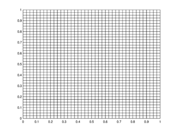
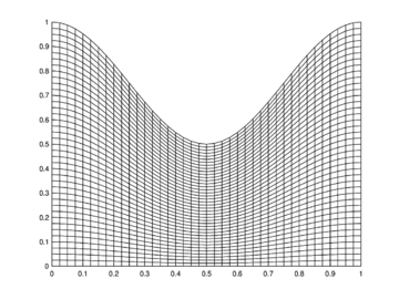
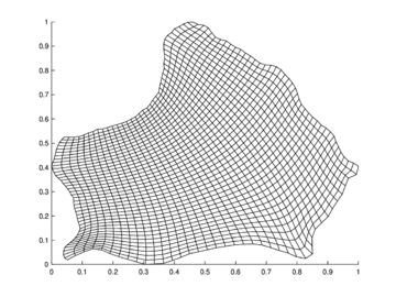
For the numerical tests, three different regions were selected: The unit square for the classical finite difference-finite volume hybrid scheme (denoted as QUAD), a widely used geometry denoted as DOME [16], that is a concave region limited by the lines ${\textstyle x=0}$ , ${\textstyle x=1}$ , ${\textstyle y=0}$ and ${\textstyle y={\frac {3}{4}}+{\frac {1}{4}}\sin {\left(\pi \left({\frac {1}{2}}-2x\right)\right)}}$ and an approximation to Zirahuen's Lake in Mexico (an endorheic basin), denoted as ZIRA. The corresponding normalized meshes with ${\textstyle 40\times {40}}$ cells can be seen in figures (4-6).

Figure 4: Regular mesh for the unitary square.

Figure 5: Mesh for DOME region.

Figure 6: Mesh for Zirahuen's Lake region.

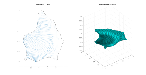
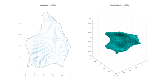
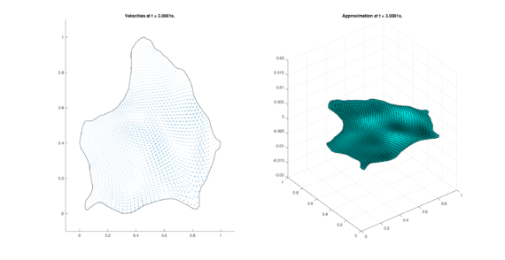
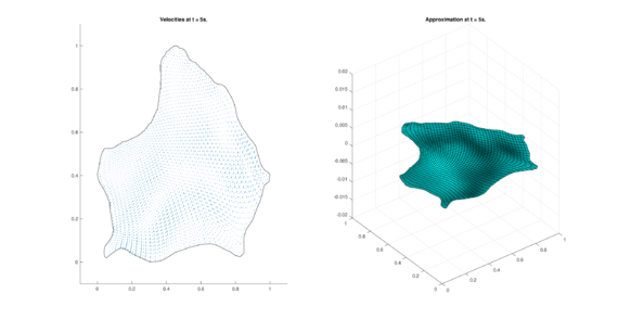
For each region 2 different tests were done, the first one using the proposed scheme for the conservative form of the Equations, and the second using the scheme for the non-conservative form.

The initial condition, for both tests, for ${\textstyle q}$ was chosen to be a droplet with different center, according to the region, as follows:

QUAD: center in ${\textstyle (.5,.3)}$ .
DOME: center in ${\textstyle (.2,.4)}$
ZIRA: center in ${\textstyle (.35,.4)}$ .

The initial conditions for ${\textstyle r}$ and ${\textstyle s}$ where fixed as ${\textstyle 0}$ for all the regions. Also, reflective boundary conditions were chosen for ${\textstyle r}$ and ${\textstyle s}$ .

To produce stable calculations [17], the time discretization was chosen by considering

where ${\textstyle \min \Delta x}$ and ${\textstyle \min \Delta y}$ are the minimum values of ${\textstyle \Delta x}$ and ${\textstyle \Delta y}$ over the region and ${\textstyle c=0.5{\frac {t}{d}}}$ . With this, the time interval ${\textstyle (0s,5s)}$ was divided into ${\textstyle 50,000}$ steps.

The total amounts of mass and momentum, over all the domain, are given at a time step ${\textstyle k}$ as

and

In our case, they were approximated by means of a numerical quadrature.

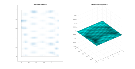
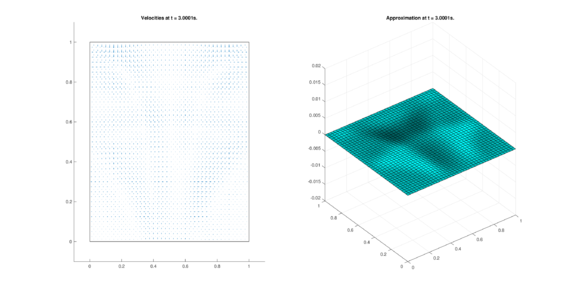
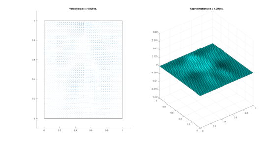
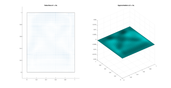
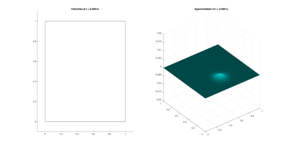
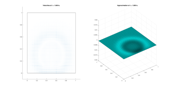
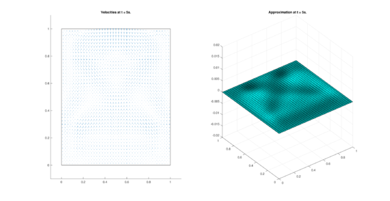
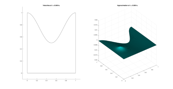
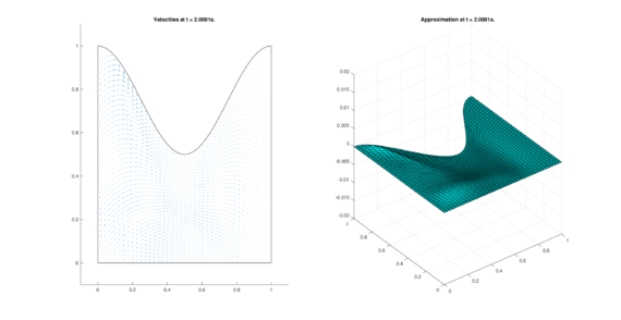
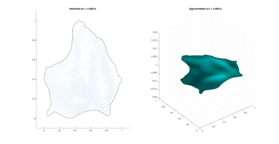
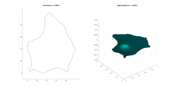
The set of figures (7) and (8) show the results for the test using the conservative form of the equations in QUAD region, while the set of figures (9) and (10) show the results non-conservative form one for the same region. Following the same idea, the results for the region DOME are shown in the sets of figures (11) to (14), the same for ZIRA region in the sets (15) to (18). These sets of figures are shown as follows: the figures on the left show the behavior of the velocities while the figures on the right show the movement of the water. The figures begin showing the second time step (t = 0.001s) and continue with a plot every of the results every second after (t = 1s, t = 2s, t = 3s, t = 4s, t = 5s).

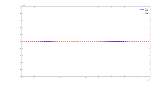
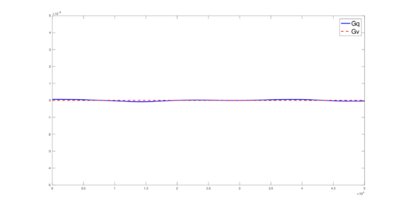
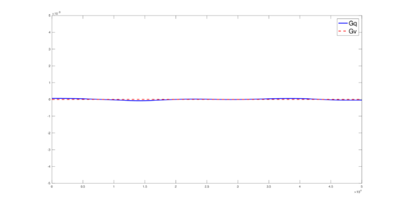
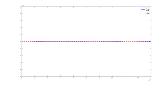
Figures (19) to (21) show the result of the computed total amount of conservative quantities over all the time steps. In all these figures the blue line represents the total amount of mass while the red-dotted line represents the total amount of momentum.


(7) Results for QUAD in the conservative case.


(8) Results for QUAD in the conservative case.


(9) Results for QUAD in the non-conservative case.


(10) Results for QUAD in the non-conservative case.


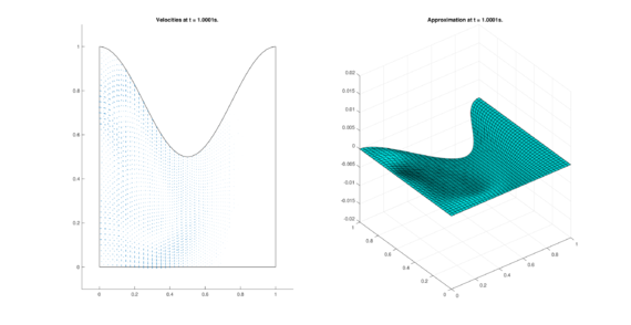
(11) Results for DOME in the conservative case.


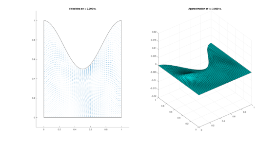
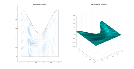
(12) Results for DOME in the conservative case.


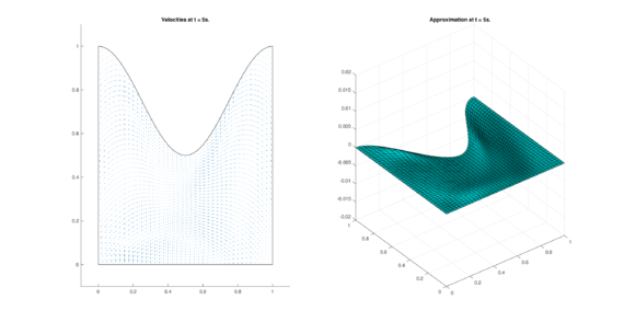
(13) Results for DOME in the non-conservative case.


(14) Results for DOME in the non-conservative case.


(15) Results for ZIRA in the conservative case.


(16) Results for ZIRA in the conservative case.


(17) Results for ZIRA in the non-conservative case.


(18) Results for ZIRA in the non-conservative case.


(19) $G_{q}$ and $G_{v}$ for QUAD.


(20) $G_{q}$ and $G_{v}$ for DOME.


(21) $G_{q}$ and $G_{v}$ for ZIRA.

It must be pointed out that, in figures (19) to (21), the conservation of mass and momentum can be appreciated, since the losses and gains of these conservative quantities, over all the computed time, is small (around ${\textstyle 10^{-5}}$ ).

4 Conclusions and future work

Figures (19) to (21) show that, with the criteria used to select ${\textstyle \Delta t}$ , neither spurious oscillations nor instabilities are observed in the tests. Even when these schemes can be applied to non-rectangular regions with ease, the quality of the grid is an important issue that must be taken into account; it is convenient to have quality grids to obtain better results, in all the tests of the present work quality grids were used.

It is important to remark that, in the tests, the boundary conditions where selected to be reflective and the tests show that, both proposed Generalized Finite Difference-Volume hybrid schemes, show a remarkable ability to produce stable results in the selected regions, even in the irregular cases; the numerical tests show that the conservation laws (mass and momentum) are fulfilled, correctly reflecting the expected behavior of a water body. As future work, these schemes need to be implemented in more realistic scenarios, which include inflows, outflows and non-slip boundary conditions.

Acknowledgments

We want to thank AULA CIMNE-Morelia and Finnish Government Scholarship Pool KM-17-10397 for the financial support for this work. We are grateful to the University of Helsinki for giving all the necessary work materials and the space to work at the Department of Physics in Helsinki, Finland.

BIBLIOGRAPHY

[1] C. B. Vreugdenhil. (1994) "Numerical Methods for Shallow-Water Flow". Springer

[2] Po-Wei Li and Chia-Ming Fan. (2017) "Generalized Finite Difference Method for Two-Dimensional Shallow Water Equations", Volume 80. Engineering Analysis with Boundary Elements 58-71

[3] C. K. Chou and C. P. Sun and D. L. Young and J. Sladek and V. Sladek. (2015) "Extrapolated Local Radial Basis Function Collocation Method for Shallow Water Problems", Volume 50. Engineering Analysis with Boundary Elements 275-290

[4] C. P. Sun and D. L. Young and T. F. Chen and C. C. Hsian. (2013) "Application of Localized Meshless Methods to 2D Shallow Water Equation Problems", Volume 37. Engineering Analysis with Boundary Elements 1339-1350

[5] Ulrik Skre Fjordholm and Siddhartha Mishra. (2012) "Accurate numerical discretizations of non-conservative hyperbolic systems", Volume 46. ESAIM: Mathematical Modelling and Numerical Analysis 1 187-206

[6] Bruno Gabutti. (1983) "On Two Upwind Finite-Difference Schemes for Hyperbolic Equations in Non-Conservative Form", Volume 11. Computers & Fluids 3 207 - 230

[7] Carlos Parés. (2006) "Numerical Methods for Nonconservative Hyperbolic Systems: A Theoretical Framework", Volume 44. SIAM Journal on Numerical Analysis 1 300-321

[8] Francisco Javier Domínguez-Mota and Pablo Michel Fernández-Valdez and Erika Ruiz-Díaz and Gerardo Tinoco-Guerrero and José Gerardo Tinoco-Ruiz. (2014) "An Heuristic Finite Difference Scheme on Irregular Plane Regions", Volume 8. Applied Mathematical Sciences 14 671-683

[9] Francisco Javier Domínguez-Mota and Sanzon Mendoza-Armenta and José Gerardo Tinoco-Ruiz. (2011) "Finite Difference Schemes Satisfying an Optimality Condition", Volume 17. IMACS. IMACS. MASCOT11 Proceedings 195

[10] Francisco Javier Domínguez-Mota and José Gerardo Tinoco-Ruiz and Gerardo Tinoco-Guerrero and Pablo Michel Fernández-Valdez and Erika Ruiz-Díaz. (2012) "A Modified Lax-Wendroff Scheme for Irregular 2D Space Regions", Volume 18. MASCOT12 Proceedings 101-110

[11] Gerardo Tinoco-Guerrero and Francisco Javier Domínguez-Mota and Ariana Gaona-Arias and Martha Leticia Ruiz-Zavala and José Gerardo Tinoco-Ruiz. (2018) "A Stability Analysis for a Generalized Finite-Difference Scheme Applied to the Pure Advection Equation", Volume 147. Mathematics and Computers in Simulation 293-300

[12] Gerardo Tinoco-Guerrero and Francisco Javier Domínguez-Mota and José Gerardo Tinoco-Ruiz and Erika Ruiz-Díaz. (2013) "An Implicit Modified Lax-Wendroff Scheme for Irregular 2D Space Regions", Volume 19. MASCOT13 Proceedings

[13] Gerardo Tinoco-Guerrero and Francisco Javier Domínguez-Mota and José Gerardo Tinoco-Ruiz and Erika Ruiz-Díaz. (2015) "Stability Aspects of a Modified Lax-Wendroff Scheme for Irregular 2D Regions", Volume 20. MASCOT15 Proceedings 161-170

[14] John C. Strikwerda. (2004) "Finite Difference Schemes and Partial Differential Equations". Society for Industrial and Applied Mathematics

[15] J. W. Thomas. (1998) "Numerical Partial Differential Equations: Finite Difference Methods". Springer

[16] Joe F. Thompson and Bharat K. Soni and Nigel P. Weatherill. (1999) "Handbook of Grid Generation". CRC Press 239 - 240

[17] Francisco Alcrudo and Pilar García-Navarro. (1993) "A high-resolution Godunov-type scheme in finite volumes for the 2D shallow-water equations", Volume 16. International Journal of Numerical Methods in Fluids 489 - 505