Solving anisotropic Poisson problems via discrete exterior calculus

Latest revision as of 15:49, 1 March 2021

Abstract

We present a local formulation for 2D Discrete Exterior Calculus (DEC) similar to that of the Finite Element Method (FEM), which allows a natural treatment of material heterogeneity (assigning material properties element by element). It also allows us to deduce, in a principled manner, anisotropic fluxes and the DEC discretization of the pullback of 1-forms by the anisotropy tensor, i.e. we deduce the discrete action of the anisotropy tensor on primal 1-forms. Due to the local formulation, the computational cost of DEC is similar to that of the Finite Element Method with Linear interpolating functions (FEML). The numerical DEC solutions to the anisotropic Poisson equation show numerical convergence, are very close to those of FEML on fine meshes and are slightly better than those of FEML on coarse meshes.

1. Introduction

The theory of Discrete Exterior Calculus (DEC) is a relatively recent discretization [8] of the classical theory of Exterior Differential Calculus developed by E. Cartan [3], which is a fundamental tool in Differential Geometry and Topology. The aim of DEC is to solve partial differential equations preserving their geometrical and physical features as much as possible. There are only a few papers about implementions of DEC to solve certain PDEs, such as the Darcy flow and Poisson's equation [9], the Navier-Stokes equations [10], the simulation of elasticity, plasticity and failure of isotropic materials [5], some comparisons with the finite differences and finite volume methods on regular flat meshes [7], as well as applications in digital geometry processing [4].

In this paper, we describe a local formulation of DEC which is reminiscent of that of the Finite Element Method (FEM). Indeed, once the local systems of equations have been established, they can be assembled into a global linear system. This local formulation is also efficient and helpful in understanding various features of DEC that can otherwise remain unclear if one is dealing dealing with an entire mesh. Besides, we believe the local description to DEC will be accesible to a wide readership. We will, therefore, take a local approach when recalling all the objects required by 2D DEC [6]. Our main results are the following:

We present a local formulation of DEC analogous to that of FEM, which allows a natural treatment of heterogeneous material properties assigned to subdomains (element by element) and eliminates the need of dealing with it through ad hoc modifications of the global discrete Hodge star operator.

Guided by the local formulation, we deduce a natural way to approximate the flux/gradient-vector of a discretized function, as well as the anisotropic flux vector. We carry out a comparison of the formulas defining the flux in both DEC and Finite Element Method with linear interpolation functions (FEML).

In order to understand how to discretize the anisotropic Poisson equation, we develop the discretization of the pull-back operator of 1-forms under an arbitrary linear trasformation or tensor. The pull-back operator is one of the basic ingredients in Exterior Differential Calculus in the smooth setting and is essential in all of its applications in Topology [bott-Tu]. We discretize the pullback operator on primal 1-forms induced by an arbitrary tensor using Whitney interpolation (the Whitney map). The Whitney interpolation forms were introduced by Hassler Whitney in 1957 [12] and Bossavit [1] explained their relevance in “mixed methods” of finite elements. To our knowledge, this is the first time that the discrete version of this operator is presented in the DEC literature. This has allowed us to discretize, in a principled manner, the anisotropic heat equation.

We carry out an analytic comparison of the DEC and FEML local formulations of the anisotropic Poisson equation.

We present three numerical examples of the approximate solutions to the stationary anisotropic Poisson equation on different domains using DEC and FEML. The numerical DEC-solutions exhibit numerical convergence (see the error measurement tables) and a competitive performance, as well as a computational cost similar to that of FEML. In fact, the numerical solutions with both methods on fine meshes are identical, and DEC shows a slightly better performance than FEML on coarse meshes.

The paper is organized as follows. In Section 2, we describe the local versions of the discrete derivative operator, the dual mesh, the discrete Hodge star operator and the meaning of a continuous 1-form on the plane. In Section 3, we deduce the discretization of the pullback operator on primal 1-forms. In Section 4, we deduce the natural way of computing flux vectors in DEC (which turns out to be equivalent to the FEML result), as well as the anisotropic flux vectors. In Section 5, we present the local DEC formulation of the 2D anisotropic Poisson equation and compare it with the local system of FEML, proving that the diffusion terms are identical in both schemes, while the source terms are differentl due to a different area-weight assignment for the nodes. In Section 6, we re-examine the geometry of some of the local DEC quantities. In Section 7, we present and compare numerical examples of DEC and FEML approximate solutions to the 2D anisotropic Poisson equation on different domains with meshes of various resolutions. In Section 8, we summarize the contributions of this paper.

2. Preliminaries on DEC from a local viewpoint

In this section, we will recall the basic operators of Dicrete Exterior Calculus restricting ourselves to a mesh made up of one simplex/triangle. The local results we derive in the paper can be assembled, just as in the Finite elemnt Method, due to the additivity of both differentiation and integration.

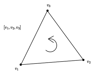
Let us consider a primal mesh made up of a single (positively oriented) triangle with vertices ${\textstyle v_{1},v_{2},v_{3}}$ (Figure 1).

Figure 1. Triangle

Such a mesh has

one oriented 2-dimensional face

three oriented 1-dimensional edges

and three 0-dimensional vertices

2.1 Boundary operator

There is a well known boundary operator

(1)

which describes the boundary of the triangle as an alternated sum of its ordered oriented edges ${\textstyle [v_{1},v_{2}]}$ , ${\textstyle [v_{1},v_{3}]}$ and ${\textstyle [v_{2},v_{3}]}$ .

Similarly, one can compute the boundary of each edge

$\partial _{1,0}[v_{1},v_{2}]=[v_{2}]-[v_{1}],$
$\partial _{1,0}[v_{1},v_{3}]=[v_{3}]-[v_{1}],$	(2)
$\partial _{1,0}[v_{2},v_{3}]=[v_{3}]-[v_{2}].$

If we consider

the symbol ${\textstyle [v_{1},v_{2},v_{3}]}$ as a basis vector of a 1-dimensional vector space,
the symbols ${\textstyle [v_{1},v_{2}]}$ , ${\textstyle [v_{1},v_{3}]}$ , ${\textstyle [v_{2},v_{3}]}$ as an ordered basis of a 3-dimensional vector space,
the symbols ${\textstyle [v_{1}]}$ , ${\textstyle [v_{2}]}$ , ${\textstyle [v_{3}]}$ as an ordered basis of a 3-dimensional vector space,

then the map (1), which sends the oriented triangle to a sum of its oriented edges, is represented by the matrix

while the map (2), which sends the oriented edges to sums of their oriented vertices, is represented by the matrix

2.2 Discrete derivative

It has been argued that the DEC discretization of the differential of a function is given by the transpose of the matrix of the boundary operator on edges [6,8]. More precisely, suppose we have a function discretized by its values at the vertices

Its discrete derivative, according to DEC, is

\left({\begin{array}{rrr}-1&-1&0\\1&0&-1\\0&1&1\end{array}}\right)^{T}\left({\begin{array}{l}f_{1}\\f_{2}\\f_{3}\end{array}}\right)=\left({\begin{array}{rrr}-1&1&0\\-1&0&1\\0&-1&1\end{array}}\right)\left({\begin{array}{l}f_{1}\\f_{2}\\f_{3}\end{array}}\right)

Indeed, such differences are rough approximations of the directional derivatives of ${\textstyle f}$ along the oriented edges. For instance, ${\textstyle f_{2}-f_{1}}$ is a rough approximation of the directional derivative of ${\textstyle f}$ at ${\textstyle v_{1}}$ in the direction of the vector ${\textstyle v_{2}-v_{1}}$ , i.e.,

It is precisely in this sense that, according to DEC,

the value ${\textstyle f_{2}-f_{1}}$ is assigned to the edge ${\textstyle [v_{1},v_{2}]}$ ,
the value ${\textstyle f_{3}-f_{1}}$ is assigned to the edge ${\textstyle [v_{1},v_{3}]}$ ,
and the value ${\textstyle f_{3}-f_{2}}$ is assigned to the edge ${\textstyle [v_{2},v_{3}]}$ .

Let

2.3 Dual mesh

The dual mesh of the primal mesh consisting of a single triangle is constructured as follows:

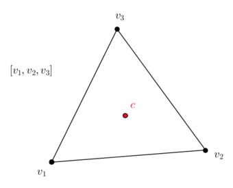
To the 2-dimensional triangular face ${\textstyle [v_{1},v_{2},v_{3}]}$ will correspond the 0-dimensional point given by the circumcenter ${\textstyle c}$ of the triangle (Figure 2).

Figure 2. Circumcenter

of the triangle

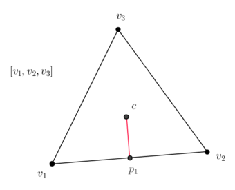
To the 1-dimensional edge ${\textstyle [v_{1},v_{2}]}$ will correspond the 1-dimensional straight line segment ${\textstyle [p_{1},c]}$ joining the midpoint ${\textstyle p_{1}}$ of the edge ${\textstyle [v_{1},v_{2}]}$ to the circumcenter ${\textstyle c}$ (Figure 3). Similarly for the other edges.

Figure 3. Dual segment

of the edge

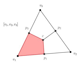
To the 0-dimensional vertex/node ${\textstyle [v_{1}]}$ will correspond the oriented ${\textstyle 2}$ -dimensional quadrilateral ${\textstyle [v_{1},p_{1},c,p_{3}]}$ (Figure 4).

Figure 4. Dual quadrilateral

of the vertex

2.4 Discrete Hodge star

For the Poisson equation in 2D, we need two matrices: one relating original edges to dual edges, and another relating vertices to dual cells.

The discrete Hodge star map ${\textstyle M_{1}}$ applied to the discrete differential of a discretized function ${\textstyle f\sim (f_{1},f_{2},f_{3})}$ is given as follows:

the value ${\textstyle f_{2}-f_{1}}$ assigned to the edge ${\textstyle [v_{1},v_{2}]}$ is changed to the new value

assigned to the segment ${\textstyle [p_{1},c]}$ ;

the value ${\textstyle f_{3}-f_{1}}$ assigned to the edge ${\textstyle [v_{1},v_{3}]}$ is changed to the new value

assigned to the edge ${\textstyle [p_{3},c]}$ .

the value ${\textstyle f_{3}-f_{2}}$ assigned to the edge ${\textstyle [v_{2},v_{3}]}$ is changed to the new value

assigned to the segment ${\textstyle [p_{2},c]}$ ;

In other words,

M_{1}=\left({\begin{array}{ccc}\displaystyle {{length}[p_{1},c] \over {length}[v_{1},v_{2}]}&0&0\\0&\displaystyle {{length}[p_{3},c] \over {length}[v_{1},v_{3}]}&0\\0&0&\displaystyle {{length}[p_{2},c] \over {length}[v_{2},v_{3}]}\end{array}}\right).

Similarly, the discrete Hodge star map ${\textstyle M_{0}}$ on values on vertices is given as follows:

the value ${\textstyle f_{1}}$ assigned to the vertex ${\textstyle [v_{1}]}$ is changed to the new value

assigned to the quadrilateral ${\textstyle [v_{1},p_{1},c,p_{3}]}$ ;

the value ${\textstyle f_{2}}$ assigned to the vertex ${\textstyle [v_{2}]}$ is changed to the new value

assigned to the quadrilateral ${\textstyle [v_{2},p_{2},c,p_{1}]}$ ;

the value ${\textstyle f_{3}}$ assigned to the vertex ${\textstyle [v_{3}]}$ is changed to the new value

assigned to the quadrilateral ${\textstyle [v_{3},p_{3},c,p_{2}]}$ .

In other words,

M_{0}=\left({\begin{array}{ccc}{Area}[v_{1},p_{1},c,p_{3}]&0&0\\0&{Area}[v_{2},p_{2},c,p_{1}]&0\\0&0&{Area}[v_{3},p_{3},c,p_{2}]\end{array}}\right).

2.5 Continuous 1-forms

A differential 1-form ${\textstyle \alpha }$ on ${\textstyle \mathbb {R} ^{2}}$ can be thought of as a function whose arguments are a point in ${\textstyle \mathbb {R} ^{2}}$ and a vector in ${\textstyle \mathbb {R} ^{2}}$ , i.e.

and which is linear on the vector argument.

The dot product of ${\textstyle \mathbb {R} ^{2}}$ allows us to see continuous 1-forms in a more familiar form as vector fields in the following way: If ${\textstyle X}$ is a vector field on ${\textstyle \mathbb {R} ^{2}}$ , at each point ${\textstyle p\in \mathbb {R} ^{2}}$ we can consider the 1-form

where ${\textstyle Y\in \mathbb {R} ^{2}}$ . On the other hand, from a continuos 1-form we can build a vector field as follows

where

2.5.1 Pullback of a conitnuous 1-form

Given a tensor ${\textstyle S}$ (a linear transformation) and the vector field ${\textstyle X}$ associated to a 1-form ${\textstyle \alpha }$ as above, consider the vector field ${\textstyle S(X)}$ . For any vector ${\textstyle Y}$ , the value of the corresponding continuous 1-form is given by the product

which is the value of the 1-form called the pullback of $\alpha$ by the tensor $S^{T}$ .

2.5.2 Discretization of continuous 1-forms

In order to produce a primal 1-form from such a continuous 1-form we need to inegrate it along the edges of the mesh (the de Rham map). In our local description, this produces a collection of 3 numbers associated to the 3 oriented edges of the triangle, i.e. for the oriented edge joining ${\textstyle v_{i}}$ to ${\textstyle v_{j}}$ we have

This is equivalent to calculating the line integral (circulation) of the corresponding vector field ${\textstyle X}$ along the path ${\textstyle \gamma _{ij}:=v_{i}+t(v_{j}-v_{i})}$ , ${\textstyle 0\leq t\leq 1}$ , parametrizing the edge ${\textstyle [v_{i},v_{j}]}$

3. Pullback operator on primal 1-forms

In Section 2, we dealt with the primal discretization of a continuous 1-form. Now we wish to understand the pullback of a primal 1-form. In order to do this, we will interpolate a primal 1-form using the Whitney interpolation forms to produce a continuous 1-form (Whitney map) to which we can apply the pullback operator by a tensor (linear transformation), and then intergrate along the edges (de Rham map).

The Whitney interpolation forms were introduced by Whitney in 1957 [12], and Bossavit [1] explained their relevance to “mixed methods” of finite elements. For the sake of simplicity, we will only define the Whitney 0 and 1-forms.

First consider the Finite Element linear basis functions (or Whitney interpolation functions)

$N_{1}={1 \over 2A}[(y_{2}-y_{3})x+(x_{3}-x_{2})y+x_{2}y_{3}-x_{3}y_{2}],$
$N_{2}={1 \over 2A}[(y_{3}-y_{1})x+(x_{1}-x_{3})y+x_{3}y_{1}-x_{1}y_{3}],$	(3)
$N_{3}={1 \over 2A}[(y_{1}-y_{2})x+(x_{2}-x_{1})y+x_{1}y_{2}-x_{2}y_{1}],$

and their differentials

$dN_{1}={1 \over 2A}[(y_{2}-y_{3})dx+(x_{3}-x_{2})dy],$
$dN_{2}={1 \over 2A}[(y_{3}-y_{1})dx+(x_{1}-x_{3})dy],$	(4)
$dN_{3}={1 \over 2A}[(y_{1}-y_{2})dx+(x_{2}-x_{1})dy].$

The Whitney interpolation 1-forms are

$\phi _{12}=N_{1}dN_{2}-N_{2}dN_{1},$
$\phi _{13}=N_{1}dN_{3}-N_{3}dN_{1},$	(5)
$\phi _{23}=N_{2}dN_{3}-N_{3}dN_{2}.$

These differential 1-forms are such that, along the edge ${\textstyle [v_{k},v_{l}]}$

i.e. ${\textstyle 0}$ or ${\textstyle \pm 1}$ .

Now, suppose we have a primal 1-form given on our triangle by the collection of numbers

We form a continuous 1-form as follows

which is such that, for ${\textstyle 1\leq i<j\leq 3}$

Now we will calculate

for an arbitrary linear transformation

Let

and

As it turns out,

where

\eta _{1}(S(w_{1}))=\left|{\begin{array}{cc}x_{3}-x_{2}&y_{3}-y_{2}\\a(x_{2}-x_{1})+b(y_{2}-y_{1})&c(x_{2}-x_{1})+d(y_{2}-y_{1})\end{array}}\right|,

\eta _{1}(S(w_{2}))=\left|{\begin{array}{cc}x_{3}-x_{2}&y_{3}-y_{2}\\a(x_{3}-x_{1})+b(y_{3}-y_{1})&c(x_{3}-x_{1})+d(y_{3}-y_{1})\end{array}}\right|,

\eta _{1}(S(w_{3}))=\left|{\begin{array}{cc}x_{3}-x_{2}&y_{3}-y_{2}\\a(x_{3}-x_{2})+b(y_{3}-y_{2})&c(x_{3}-x_{2})+d(y_{3}-y_{2})\end{array}}\right|,

\eta _{2}(S(w_{1}))=\left|{\begin{array}{cc}x_{1}-x_{3}&y_{1}-y_{3}\\a(x_{2}-x_{1})+b(y_{2}-y_{1})&c(x_{2}-x_{1})+d(y_{2}-y_{1})\end{array}}\right|,

\eta _{2}(S(w_{2}))=\left|{\begin{array}{cc}x_{1}-x_{3}&y_{1}-y_{3}\\a(x_{3}-x_{1})+b(y_{3}-y_{1})&c(x_{3}-x_{1})+d(y_{3}-y_{1})\end{array}}\right|,

\eta _{2}(S(w_{3}))=\left|{\begin{array}{cc}x_{1}-x_{3}&y_{1}-y_{3}\\a(x_{3}-x_{2})+b(y_{3}-y_{2})&c(x_{3}-x_{2})+d(y_{3}-y_{2})\end{array}}\right|,

\eta _{3}(S(w_{1}))=\left|{\begin{array}{cc}x_{2}-x_{1}&y_{2}-y_{1}\\a(x_{2}-x_{1})+b(y_{2}-y_{1})&c(x_{2}-x_{1})+d(y_{2}-y_{1})\end{array}}\right|,

\eta _{3}(S(w_{2}))=\left|{\begin{array}{cc}x_{2}-x_{1}&y_{2}-y_{1}\\a(x_{3}-x_{1})+b(y_{3}-y_{1})&c(x_{3}-x_{1})+d(y_{3}-y_{1})\end{array}}\right|,

\eta _{3}(S(w_{3}))=\left|{\begin{array}{cc}x_{2}-x_{1}&y_{2}-y_{1}\\a(x_{3}-x_{2})+b(y_{3}-y_{2})&c(x_{3}-x_{2})+d(y_{3}-y_{2})\end{array}}\right|.

Anyhow, these quantities are areas of the parallelograms formed by one fixed edge of the original triangle and one edge transformed by ${\textstyle S}$ .

Thus, we have that the induced transformation on primal 1-forms is

S^{*}\beta ={1 \over 4A}\left({\begin{array}{ccc}\eta _{2}(S(w_{1}))-\eta _{1}(S(w_{1}))&\eta _{3}(S(w_{1}))&\eta _{3}(S(w_{1}))\\\eta _{2}(S(w_{2}))&\eta _{3}(S(w_{2}))-\eta _{1}(S(w_{2}))&-\eta _{2}(S(w_{2}))\\-\eta _{1}(S(w_{3}))&-\eta _{1}(S(w_{3}))&\eta _{3}(S(w_{3}))-\eta _{2}(S(w_{3}))\end{array}}\right)\left({\begin{array}{c}\beta _{12}\\\beta _{13}\\\beta _{23}\end{array}}\right)

(6)

When the material is isotropic, i.e. ${\textstyle S}$ is a constant multiple of the ${\textstyle 2\times 2}$ identity matrix, we get a constant multiple of the ${\textstyle 3\times 3}$ identity matrix above as discrete pull-back operator.

4. Flux and anisotropy

In this section, we deduce the DEC formulae for the local flux, the local anisotropic flux and the local anisotropy operator for primal 1-forms.

4.1 The flux in local DEC

We wish to find a natural construction for the discrete flux (discrete gradient vector) of a discrete function. Recall from Vector Calculus that the directional derivative of a differentiable function ${\textstyle f:\mathbb {R} ^{2}\longrightarrow \mathbb {R} }$ at a point ${\textstyle p\in \mathbb {R} ^{2}}$ in the direction of ${\textstyle w\in \mathbb {R} ^{2}}$ is defined by

Thus, we have three Vector Calculus identities

As in Subsection 2.2, the rough approximations to directional derivatives of a function ${\textstyle f}$ in the directions of the (oriented) edges are given as follows

Thus, if we want to find a discrete gradient vector ${\textstyle W_{1}}$ of ${\textstyle f}$ at the point ${\textstyle v_{1}}$ , we need to solve the equations

$W_{1}\cdot (v_{2}-v_{1})=f_{2}-f_{1}$	(7)
$W_{1}\cdot (v_{3}-v_{1})=f_{3}-f_{1}.$	(8)

If

then

W_{1}=\left({f_{1}y_{2}-f_{1}y_{3}-f_{2}y_{1}+f_{2}y_{3}+f_{3}y_{1}-f_{3}y_{2} \over x_{1}y_{2}-x_{1}y_{3}-x_{2}y_{1}+x_{2}y_{3}+x_{3}y_{1}-x_{3}y_{2}},-{f_{1}x_{2}-f_{1}x_{3}-f_{2}x_{1}+f_{2}x_{3}+f_{3}x_{1}-f_{3}x_{2} \over x_{1}y_{2}-x_{1}y_{3}-x_{2}y_{1}+x_{2}y_{3}+x_{3}y_{1}-x_{3}y_{2}}\right)^{T}

Now, if we were to find a discrete gradient vector ${\textstyle W_{2}}$ of ${\textstyle f}$ at the point ${\textstyle v_{2}}$ , we need to solve the equations

$W_{2}\cdot (v_{1}-v_{2})=f_{1}-f_{2}$	(9)
$W_{2}\cdot (v_{3}-v_{2})=f_{3}-f_{2}.$

The vectors ${\textstyle W_{2}}$ solving these equations is actually equal to ${\textstyle W_{1}}$ . Indeed, consider

so that

(10)

Thus, adding up (7) and (9) we get

(11)

Subtracting (8) from (10) we get

(12)

Since ${\textstyle v_{2}-v_{1}}$ and ${\textstyle v_{3}-v_{2}}$ are linearly independent and the two inner products in (11) and (12) vanish,

Analogously, the corresponding gradient vector ${\textstyle W_{3}}$ of ${\textstyle f}$ at the vertex ${\textstyle v_{3}}$ is equal to ${\textstyle W_{1}}$ . This means that the three approximate gradient vectors at the three vertices coincide, i.e. we have a unique discrete flux vector ${\textstyle W=W_{1}=W_{2}=W_{3}}$ on the given element. Note that the discrete flux ${\textstyle W}$ satisfies

This means that the primal 1-form discretizing ${\textstyle df}$ can be obtained by performing the dot products of the discrete flux vector ${\textstyle W}$ with the vectors given by the triangle's oriented edges.

4.1.1 Comparison of DEC and FEML local fluxes

The local flux (gradient) of ${\textstyle f}$ in FEML is given by

\left({\begin{array}{ccc}\displaystyle {\partial N_{1} \over \partial x}&\displaystyle \displaystyle {\partial N_{2} \over \partial x}&\displaystyle {\partial N_{3} \over \partial x}\\\displaystyle {\partial N_{1} \over \partial y}&\displaystyle {\partial N_{2} \over \partial y}&\displaystyle {\partial N_{3} \over \partial y}\end{array}}\right)\left({\begin{array}{c}f_{1}\\f_{2}\\f_{3}\end{array}}\right),

where ${\textstyle N_{1},N_{2}}$ and ${\textstyle N_{3}}$ are the basis functions given in (3). Explicitly

\left({\begin{array}{ccc}\displaystyle {\partial N_{1} \over \partial x}&\displaystyle {\partial N_{2} \over \partial x}&\displaystyle {\partial N_{3} \over \partial x}\\\displaystyle {\partial N_{1} \over \partial y}&\displaystyle {\partial N_{2} \over \partial y}&\displaystyle {\partial N_{3} \over \partial y}\end{array}}\right)={1 \over 2A}\left({\begin{array}{ccc}y_{2}-y_{3}&y_{3}-y_{1}&y_{1}-y_{2}\\x_{3}-x_{2}&x_{1}-x_{3}&x_{2}-x_{1}\end{array}}\right)

where

is the area of the triangle, so that the FEML flux is given by

\left({[(y_{2}-y_{3})f_{1}+(y_{3}-y_{1})f_{2}+(y_{1}-y_{2})f_{3}] \over 2A},{[(x_{3}-x_{2})f_{1}+(x_{1}-x_{3})f_{2}+(x_{2}-x_{1})f_{3}] \over 2A}\right)^{T},

and we can see that it coincides with the DEC flux.

4.2 The anisotropic flux vector in local DEC

We will now discuss how to discretize anisotropy in 2D DEC. Let ${\textstyle K}$ denote the symmetric anisotropy tensor

and recall the anisotropic Poisson equation

First recall that, in Exterior Differential Calculus, for any ${\textstyle w\in \mathbb {R} ^{2}}$ ,

where ${\textstyle K^{*}df_{p}}$ is the pullback of ${\textstyle df_{p}}$ by ${\textstyle K}$ .

Since we already have a discrete candidate ${\textstyle W}$ for ${\textstyle \nabla f}$ on the given element, the product of the matrix ${\textstyle K}$ and ${\textstyle W}$ gives us a candidate ${\textstyle W':=KW}$ for the anisptropic flux vector on such an element

W':=KW=\left({\begin{array}{cc}k_{11}&k_{12}\\k_{12}&k_{22}\end{array}}\right)\left({\begin{array}{c}{[(y_{2}-y_{3})f_{1}+(y_{3}-y_{1})f_{2}+(y_{1}-y_{2})f_{3}] \over 2A}\\{[(x_{3}-x_{2})f_{1}+(x_{1}-x_{3})f_{2}+(x_{2}-x_{1})f_{3}] \over 2A}\end{array}}\right)

=\left({\begin{array}{c}{k_{11}[f_{1}(y_{2}-y_{3})+f_{2}(y_{3}-y_{1})+f_{3}(y_{1}-y_{2})]+k_{12}[f_{1}(x_{3}-x_{2})+f_{2}(x_{1}-x_{3})+f_{3}(x_{2}-x_{1})] \over x_{1}y_{2}-x_{1}y_{3}-x_{2}y_{1}+x_{2}y_{3}+x_{3}y_{1}-x_{3}y_{2}}\\{k_{12}[f_{1}(y_{2}-y_{3})+f_{2}(y_{3}-y_{1})+f_{3}(y_{1}-y_{2})]+k_{22}[f_{1}(x_{3}-x_{2})+f_{2}(x_{1}-x_{3})+f_{3}(x_{2}-x_{1})] \over x_{1}y_{2}-x_{1}y_{3}-x_{2}y_{1}+x_{2}y_{3}+x_{3}y_{1}-x_{3}y_{2}}\end{array}}\right).

In order to produce a primal 1-form from ${\textstyle W'}$ , all we have to do is assume that ${\textstyle K}$ is constant on the given triangle and take dot products with the edges of the triangle, i.e.

Nevertheless, in order to better understand the structure of the local system (as in FEML), it is desirable to have a factorization of the result as a matrix product

where the matrix ${\textstyle K^{DEC}}$ is a real ${\textstyle 3\times 3}$ matrix depending on the geometry of the triangle and the matrix ${\textstyle K}$ , and such that it is a multiple of the identity matrix when the domain is isotropic. In order to do this, we will use the discretization of the pullback opertator of Exterior Differential Calculus for arbitrary 1-forms from Section 3. Thus, using (6), ${\textstyle K^{DEC}}$ is the following ${\textstyle 3\times 3}$ matrix where we have set ${\textstyle S=K}$ , i.e.

K^{DEC}={1 \over 4A}\left({\begin{array}{ccc}\eta _{21}^{K}-\eta _{11}^{K}&\eta _{31}^{K}&\eta _{31}^{K}\\\eta _{22}^{K}&\eta _{32}^{K}-\eta _{12}^{K}&-\eta _{22}^{K}\\-\eta _{13}^{K}&-\eta _{13}^{K}&\eta _{33}^{K}-\eta _{23}^{K}\end{array}}\right)

where

4.2.1 Geometric interpretation of the entries of $K^{DEC}$ 4.2.1 Geometric interpretation of the entries of K D E C {\displaystyle K^{DEC}}

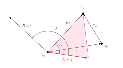
Consider the Figure 5, where ${\textstyle J}$ denotes the ${\textstyle 90^{\circ }}$ anti-clockwise rotation

Figure 5. Geometric interpretation of the entries of the anisotropy tensor discretization

We have

where ${\textstyle A'}$ is the area of the red triangle. Thus, the numbers ${\textstyle \eta _{kl}^{K}}$ are quotients of areas of transformed triangles divided by the area of the original triangle.

5. Anisotropic Poisson equation in 2D

In this section, we describe the local DEC discretization of the 2D anisotropic Poisson equation and compare it to that of FEML.

5.1 Local DEC discretization of the 2D anisotropic Poisson equation

The anisotropic Poisson equation reads as follows

where ${\textstyle f}$ and ${\textstyle q}$ are two functions on a certain domain in ${\textstyle \mathbb {R} ^{2}}$ and ${\textstyle K}$ is the anisotropy tensor. In terms of the exterior derivative ${\textstyle d}$ and the Hodge star operator ${\textstyle \star }$ it reads as follows

where ${\textstyle K^{*}df:=df\circ K}$ and ${\textstyle K=K^{T}}$ . Following the discretization of the discretized divergence operator [6], the corresponding local DEC discretization of the anisotropic Poisson equation is

or equivalently

(13)

In order to simplify the notation, consider the lengths and areas defined in Figure 6.

Figure 6. Triangle

Now, the discretized equation (13) looks as follows:

{1 \over 4A}\left({\begin{array}{ccc}1&-1&0\\-1&0&-1\\0&1&1\end{array}}\right)\left({\begin{array}{ccc}{l_{1} \over L_{1}}&0&0\\0&{l_{3} \over L_{3}}&0\\0&0&{l_{2} \over L_{2}}\end{array}}\right)\left({\begin{array}{ccc}\eta _{21}^{K}-\eta _{11}^{K}&\eta _{31}^{K}&\eta _{31}^{K}\\\eta _{22}^{K}&\eta _{32}^{K}-\eta _{12}^{K}&-\eta _{22}^{K}\\-\eta _{13}^{K}&-\eta _{13}^{K}&\eta _{33}^{K}-\eta _{23}^{K}\end{array}}\right)\left({\begin{array}{rrr}-1&1&0\\-1&0&1\\0&-1&1\end{array}}\right)\left({\begin{array}{c}f_{1}\\f_{2}\\f_{3}\end{array}}\right)=\left({\begin{array}{c}A_{1}q_{1}\\A_{2}q_{2}\\A_{3}q_{3}\end{array}}\right).

The diffusive term matrix is actually symmetric (see Subsection 5.3.1).

5.2 Local FEML-Discretized 2D anisotropic Poisson equation

The diffusive elemental matrix in FEM (frequently called “stiffness matrix”) on an element ${\textstyle e}$ is given by

where ${\textstyle D=K}$ is the matrix representing the anisotropic diffusion tensor, and the matrix ${\textstyle B}$ is given explicitly by

B=\left({\begin{array}{ccc}\displaystyle {\partial N_{1} \over \partial x}&\displaystyle {\partial N_{2} \over \partial x}&\displaystyle {\partial N_{3} \over \partial x}\\\displaystyle {\partial N_{1} \over \partial y}&\displaystyle {\partial N_{2} \over \partial y}&\displaystyle {\partial N_{3} \over \partial y}\end{array}}\right)={1 \over 2A}\left({\begin{array}{ccc}y_{2}-y_{3}&y_{3}-y_{1}&y_{1}-y_{2}\\x_{3}-x_{2}&x_{1}-x_{3}&x_{2}-x_{1}\end{array}}\right).

Since the matrix ${\textstyle B}$ is constant on an element of the mesh, the integral is easy to compute. Thus, the difussive matrix ${\textstyle K_{e}}$ for a linear triangular element (FEML) is given by

={1 \over 4A_{e}}\left({\begin{array}{ccc}y_{2}-y_{3}&x_{3}-x_{2}\\y_{3}-y_{1}&x_{1}-x_{3}\\y_{1}-y_{2}&x_{2}-x_{1}\end{array}}\right)\left({\begin{array}{cc}k_{11}&k_{12}\\k_{12}&k_{22}\end{array}}\right)\left({\begin{array}{ccc}y_{2}-y_{3}&y_{3}-y_{1}&y_{1}-y_{2}\\x_{3}-x_{2}&x_{1}-x_{3}&x_{2}-x_{1}\end{array}}\right)

Now, let us consider the first diagonal entry of the local FEML anisotropic Poisson diffusive matrix ${\textstyle K_{e}}$ ,

={1 \over 4A}({\begin{array}{cc}-(y_{3}-y_{2}),&x_{3}-x_{2}\end{array}})\left({\begin{array}{cc}k_{11}&k_{12}\\k_{12}&k_{22}\end{array}}\right)\left({\begin{array}{c}-(y_{3}-y_{2})\\x_{3}-x_{2}\end{array}}\right)

={1 \over 4A}({\begin{array}{cc}x_{3}-x_{2},&y_{3}-y_{2}\end{array}})\left({\begin{array}{cc}0&1\\-1&0\end{array}}\right)\left({\begin{array}{cc}k_{11}&k_{12}\\k_{12}&k_{22}\end{array}}\right)\left({\begin{array}{cc}0&-1\\1&0\end{array}}\right)\left({\begin{array}{c}x_{3}-x_{2}\\y_{3}-y_{2}\end{array}}\right)

where ${\textstyle J}$ is the ${\textstyle 90^{\circ }}$ anticlockwise rotation,

In this notation, the diffusive term in local FEML is given as follows

{1 \over 4A}\left({\begin{array}{ccc}J(v_{3}-v_{2})\cdot K(J(v_{3}-v_{2}))&J(v_{3}-v_{2})\cdot K(J(v_{1}-v_{3}))&J(v_{3}-v_{2})\cdot K(J(v_{2}-v_{1}))\\J(v_{1}-v_{3})\cdot K(J(v_{3}-v_{2}))&J(v_{1}-v_{3})\cdot K(J(v_{1}-v_{3}))&J(v_{1}-v_{3})\cdot K(J(v_{2}-v_{1}))\\J(v_{2}-v_{1})\cdot K(J(v_{3}-v_{2}))&J(v_{2}-v_{1})\cdot K(J(v_{1}-v_{3}))&J(v_{2}-v_{1})\cdot K(J(v_{2}-v_{1}))\end{array}}\right).

5.3 Comparison between local DEC and FEML discretizations

For the sake of brevity, we are only going to compare the entries of the first row and first column of each formulation. Consider the various lengths, areas and angles labeled in Figures 6 and 7.

Figure 7. Circumscribed triangle.

We have the following identities:

5.3.1 The diffusive term

For instance, we claim that

{J(v_{3}-v_{2})\cdot K(J(v_{3}-v_{2})) \over 4A}={1 \over 4A}\left({l_{1}(\eta _{3,1}^{K}+\eta _{2,1}^{K}-\eta _{1,1}^{K}) \over L_{1}}+{l_{3}(\eta _{3,2}^{K}+\eta _{2,2}^{K}-\eta _{1,2}^{K}) \over L_{3}}\right)

Indeed,

\eta _{3,1}^{K}+\eta _{2,1}^{K}-\eta _{1,1}^{K}=\left|{\begin{array}{cc}x_{2}-x_{1}&y_{2}-y_{1}\\dx(K(w_{1}))&dy(K(w_{1}))\end{array}}\right|+\left|{\begin{array}{cc}x_{1}-x_{3}&y_{1}-y_{3}\\dx(K(w_{1}))&dy(K(w_{1}))\end{array}}\right|-\left|{\begin{array}{cc}x_{3}-x_{2}&y_{3}-y_{2}\\dx(K(w_{1}))&dy(K(w_{1}))\end{array}}\right|

\eta _{3,2}^{K}+\eta _{2,2}^{K}-\eta _{1,2}^{K}=\left|{\begin{array}{cc}x_{2}-x_{1}&y_{2}-y_{1}\\dx(K(w_{2}))&dy(K(w_{2}))\end{array}}\right|+\left|{\begin{array}{cc}x_{1}-x_{3}&y_{1}-y_{3}\\dx(K(w_{2}))&dy(K(w_{2}))\end{array}}\right|-\left|{\begin{array}{cc}x_{3}-x_{2}&y_{3}-y_{2}\\dx(K(w_{2}))&dy(K(w_{2}))\end{array}}\right|

Thus,

{\begin{array}{l}&\displaystyle {1 \over 4A}\left(\displaystyle {l_{1}(\eta _{3,1}^{K}+\eta _{2,1}^{K}-\eta _{1,1}^{K}) \over L_{1}}+\displaystyle {l_{3}(\eta _{3,2}^{K}+\eta _{2,2}^{K}-\eta _{1,2}^{K}) \over L_{3}}\right)=\\&\qquad =-\displaystyle {1 \over 2A}\left(\displaystyle {l_{1} \over L_{1}}J(v_{3}-v_{2})\cdot K(v_{2}-v_{1})+\displaystyle {l_{1} \over L_{1}}J(v_{3}-v_{2})\cdot K(v_{3}-v_{1})\right)\\&\qquad =\displaystyle {J(v_{3}-v_{2})\cdot K(v_{1}-v_{3}) \over 2A}{\tan(\alpha _{3}) \over 2}-\displaystyle {J(v_{3}-v_{2})\cdot K(v_{2}-v_{1}) \over 2A}\displaystyle {\tan(\alpha _{1}) \over 2}\\&\qquad =\displaystyle {1 \over 4A}J(v_{3}-v_{2})\cdot K((v_{1}-v_{3})\tan(\alpha _{3})-(v_{2}-v_{1})\tan(\alpha _{1})).\end{array}}

All we have to do now is show that

Note that, since ${\textstyle J(v_{3}-v_{2})}$ is orthogonal to ${\textstyle v_{3}-v_{2}}$ , ${\textstyle J(v_{3}-v_{2})}$ must be parallel to ${\textstyle c-{v_{2}+v_{3} \over 2}}$ . Thus,

(14)

Now we are going to express ${\textstyle c}$ in terms of ${\textstyle v_{1},v_{2},v_{3}}$ . Let us consider

where ${\textstyle a,b}$ are coefficients to be determined. Taking inner products with ${\textstyle (v_{2}-v_{1})}$ and ${\textstyle (v_{3}-v_{1})}$ we get the two equations

Solving for ${\textstyle a}$ and ${\textstyle b}$

Substituting all the relevant quantities in (14) we have, for instance, that the coefficient of ${\textstyle (v_{2}-v_{1})}$ is

2{\cos(\alpha _{2}) \over \sin(\alpha _{2})}\left({\sin(\alpha _{3}) \over 2\cos(\alpha _{1})\sin(\alpha _{1}+\alpha _{3})}-{1 \over 2}\right)={\cos(\alpha _{2}) \over \sin(\alpha _{2})}\left({\sin(\alpha _{3})-\cos(\alpha _{1})\sin(\alpha _{1}+\alpha _{3}) \over \cos(\alpha _{1})\sin(\alpha _{1}+\alpha _{3})}\right)

={\cos(\alpha _{2}) \over \sin(\alpha _{2})}\left({\sin(\alpha _{3})-\cos(\alpha _{1})(\sin(\alpha _{1})\cos(\alpha _{3})+\sin(\alpha _{3})\cos(\alpha _{1})) \over \cos(\alpha _{1})\sin(\pi /2-\alpha _{2})}\right)

and similarly for the coefficient of ${\textstyle (v_{1}-v_{3})}$ . The calculations for the remaining entries are similar.

Thus, the local DEC and FEML diffusive terms of the 2D anisotropic Poisson equation coincide.

5.3.2 The source term

As already observed in [6], the right hand sides of the local DEC and FEML systems are different

While FEML uses a barycentric subdivision to calculate the areas associated to each node/vertex, DEC uses a circumcentric subdivision. Eventually, this leads the DEC discretization to a better approximation of the solution (on coarse meshes).

6. Some remarks about DEC quantities

6.1 The discrete Hodge star quantities revisited

The numbers appearing in the local DEC matrices can be expressed both in terms of determinants and in terms of trigonometric functions. More precisely,

A_{1}={1 \over 4}\left[\det \left({\begin{array}{ccc}x_{1}&y_{1}&1\\x_{c}&y_{c}&1\\x_{2}&y_{2}&1\end{array}}\right)+\det \left({\begin{array}{ccc}x_{3}&y_{3}&1\\x_{c}&y_{c}&1\\x_{1}&y_{1}&1\end{array}}\right)\right]\quad =\quad {R^{2} \over 4}(\sin(2\alpha _{1})+\sin(2\alpha _{3})),

A_{2}={1 \over 4}\left[\det \left({\begin{array}{ccc}x_{1}&y_{1}&1\\x_{c}&y_{c}&1\\x_{2}&y_{2}&1\end{array}}\right)+\det \left({\begin{array}{ccc}x_{2}&y_{2}&1\\x_{c}&y_{c}&1\\x_{3}&y_{3}&1\end{array}}\right)\right]\quad =\quad {R^{2} \over 4}(\sin(2\alpha _{1})+\sin(2\alpha _{2})),

A_{3}={1 \over 4}\left[\det \left({\begin{array}{ccc}x_{2}&y_{2}&1\\x_{c}&y_{c}&1\\x_{3}&y_{3}&1\end{array}}\right)+\det \left({\begin{array}{ccc}x_{3}&y_{3}&1\\x_{c}&y_{c}&1\\x_{1}&y_{1}&1\end{array}}\right)\right]\quad =\quad {R^{2} \over 4}(\sin(2\alpha _{2})+\sin(2\alpha _{3})),

These expressions are valid regardless of the location of the circumcenter and can, indeed, take negative values. The angles that are measured in the scheme can be negative as in the obtuse triangle of Figure 8.


Figure 8. Negative (exterior) angles measured in an obtuse triangle

and some quantities can even be zero. For instance, if

then

6.2 Area weights assigned to vertices

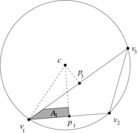
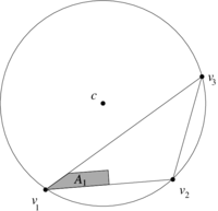
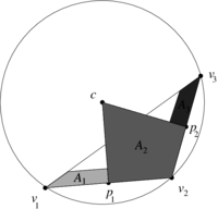
In order to understand how local DEC assigns area weights to vertices differently from FEML, let us consider the obtuse triangle shown in Figure 8. Let ${\textstyle p_{1},p_{2},p_{3}}$ be the middle points of the segments ${\textstyle [v_{1},v_{2}],[v_{1},v_{3}],[v_{2},v_{3}]}$ respectively. As shown in Figure 9, the triangle ${\textstyle [v_{1},p_{3},c]}$ lies completely outside of the triangle ${\textstyle [v_{1},v_{2},v_{3}]}$ . Geometrically, this implies that its area must be assigned a negative sign, which is confirmed by the determinant formulas of Subsection 6.1. On the other hand, the triangle ${\textstyle [v_{1},p_{1},c]}$ will have positive area. Thus, their sum gives us the area ${\textstyle A_{1}}$ in Figure 9.


Figure 9. Area weight assigned to ${\textstyle v_{1}}$

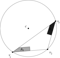
The area ${\textstyle A_{3}}$ is computed similarly, where the triangle ${\textstyle [p_{3},v_{3},c]}$ is assigned negative area (Figure 10).


Figure 10. Area weight assigned to ${\textstyle v_{3}}$

Note that for ${\textstyle A_{2}}$ , the two triangles ${\textstyle [p_{1},v_{2},c]}$ and ${\textstyle [v_{2},p_{2},c]}$ both have positive areas (Figure 11).


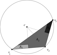
Figure 11. Area weight assigned to ${\textstyle v_{2}}$

7. Numerical examples

In this section, we present three numerical examples in order to illustrate the performance of DEC resulting from the local formulation and its implementation. In all cases, we solve the anisotropic Poisson equation. The FEML methodology that we have used in the comparison can be consulted [2,11,13].

7.1 First example: Heterogeneity

This example is intended to highlight how Local DEC deals effectively with heterogeneous materials. Consider the region in the plane given in Figure 12.

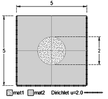
Figure 12. Square and inner circle with different conditions

The difussion constant for the region labelled mat1 is ${\textstyle k=12}$ and its source term is ${\textstyle q=20}$ .
The difussion constant for the region labelled mat2 is ${\textstyle k=6}$ and its source term is ${\textstyle q=5}$ .

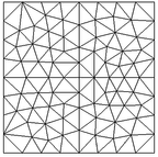
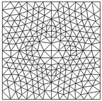
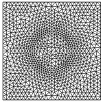
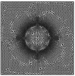
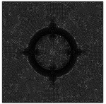
The meshes used in this example are shown in Figure 13 and vary from coarse to very fine.


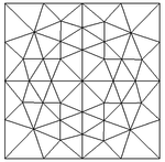
(a)	(b)	(c)

(d)	(e)	(f)
Figure 13. Six of the meshes used in the first example

The numerical results for the maximum temperature value are exemplified in Table 1.

Table 1. Numerical simulation results of the first example

Mesh	Nodes	Elements	Max. Temp. Value		Max. Flux Magnitude
Mesh	Nodes	Elements	DEC	FEML	DEC	FEML
Figure 13(a)	49	80	5.51836	5.53345	13.837	13.453
Figure 13(b)	98	162	5.65826	5.66648	14.137	14.024
Figure 13(c)	258	466	5.70585	5.71709	14.858	14.770
Figure 13(d)	1,010	1,914	5.72103	5.72280	15.008	15.006
Figure 13(e)	3,813	7,424	5.72725	5.72725	15.229	15.228
Figure 13(f)	13,911	27,420	5.72821	5.72826	15.342	15.337
	50,950	101,098	5.72841	5.72842	15.395	15.396
	135,519	269,700	5.72845	5.72845	15.420	15.417
	298,299	594,596	5.72848	5.72848	15.430	15.429
	600,594	1,198,330	5.72848	5.72848	15.433	15.433
	1,175,238	2,346,474	5.72849	5.72849	15.43724	15.43724

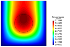
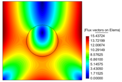
The temperature and flux-magnitude distribution fields are shown in Figure 14.


(a) Contour fill of temperatures	(b) Contour fill of flux vectors on Elems
Figure 14. Temperature and flux-magnitude distribution fields of the first example

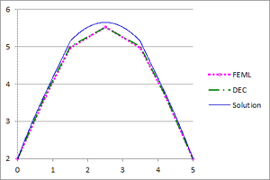
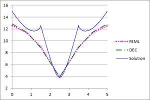
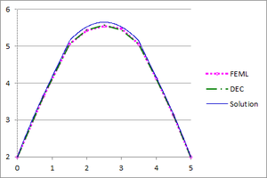
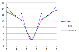
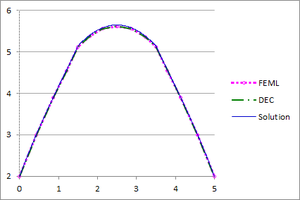
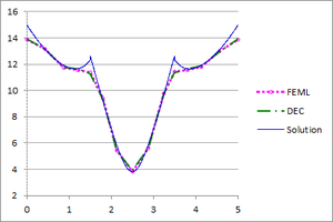
Figure 15 shows the graphs of the temperature and the flux-magnitude along a horizontal line crossing the inner circle for the first two meshes.


(a)	(b)

(c)	(d)

(e)	(f)
Figure 15. Temperature and Flux magnitude graphs of the first example along a cross-section of the domain for different meshes

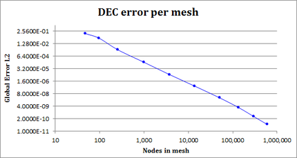
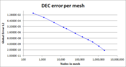
Table 2 shows some global error metrics for different meshes. Figure 16 shows the error evolution in ${\textstyle L^{2}}$ norm for this example.

Table 2. DEC

errors in the first example

Mesh	Nodes	${\sum (u-u_{i})^{2} \over nodes}$	$L^{2}$ norm
1	49	1.0537e-02	1.4438e-01
2	98	4.2447e-03	4.8558e-02
3	258	6.9781e-04	3.0390e-03
4	1,010	8.8386e-05	1.4877e-04
5	3,813	1.0736e-05	7.7369e-06
6	13,911	1.4422e-06	4.9791e-07
7	50,950	1.7582e-07	2.9608e-08
8	135,518	3.2621e-08	2.9233e-09
9	298,299	7.3566e-09	3.3610e-10
10	603,440	1.8577e-09	4.9496e-11

Figure 16. DEC

error in the first example

7.2 Second example: Anisotropy

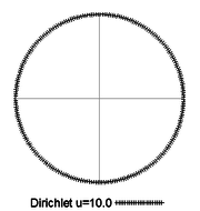
Let us solve the Poisson equation in a circle of radius one centered at the origin ${\textstyle (0,0)}$ under the following conditions (Figure 17):

heat anisotropic diffusion constants ${\textstyle K_{x}=1.5,K_{y}=1.0}$ ;
material angle ${\textstyle 30^{\circ }}$ ;
source term ${\textstyle q=1}$ ;
Dirichlet boundary condition ${\textstyle u=10}$ .

Figure 17. Disk of radius one

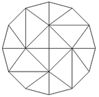
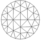
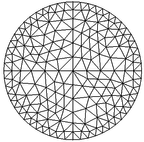
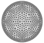
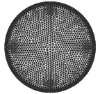
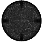
The meshes used in this example are shown in Figure 18 and vary from very coarse to very fine.


(a)	(b)	(c)

(d)	(e)	(f)
Figure 18. First six meshes used for unit disk

The numerical results for the maximum temperature value ( ${\textstyle u(0,0)=10.2}$ ) are exemplified in Table 3 where a comparison with the Finite Element Method with linear interpolation functions (FEML) is also shown.

Table 3. Temperature value at the point (0,0) and Flux magnitude value at the point (-1, 0) of the numerical simulations for the second example

Mesh	Nodes	Elements	Temp. Value at $(0,0)$		Flux Magnitude at $(-1,0)$
Mesh	Nodes	Elements	DEC	FEML	DEC	FEML
Figure 18(a)	17	20	10.20014	10.19002	0.42133	0.43865
Figure 18(b)	41	56	10.20007	10.19678	0.48544	0.49387
Figure 18(c)	201	344	10.20012	10.20158	0.52470	0.52428
Figure 18(d)	713	1304	10.20000	10.19969	0.54143	0.54224
Figure 18(e)	2455	4660	10.20000	10.19990	0.54971	0.55138
Figure 18(f)	8180	15862	10.20000	10.20002	0.55326	0.55409
	20016	39198	10.20000	10.19999	0.55470	0.55520
	42306	83362	10.20000	10.20000	0.55540	0.55572

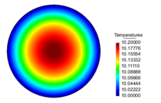
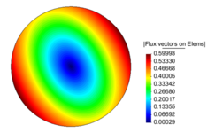
The temperature distribution and Flux magnitude fields for the finest mesh are shown in Figure 19.


(a) Contour Fill of Temperatures	(b) Contour Fill of Flux vectors on Elems
Figure 19. Temperature distribution and Flux magnitude fields for the finest mesh of the second example

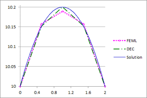
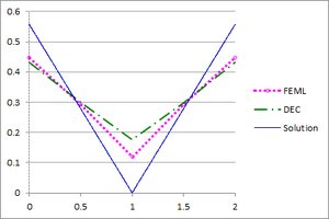
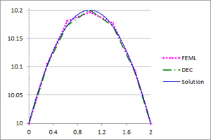
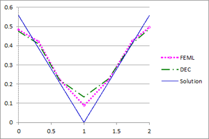
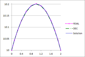
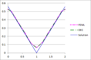
Figures 20(a), (b) and (c) show the graphs of the temperature and flux magnitude values along a diameter of the circle for the different meshes of Figures 18(a), (b) and (c), respectively.


(a)	(b)

(c)	(d)

(e)	(f)
Figure 20. Temperature and Flux magnitude graphs of the second example along a diameter of the circle for different meshes: mesh in Figure 18(a), a-Temperature, b-Flux; mesh in Figure 18(b), c-Temperature, d-Flux; mesh in Figure 18(c), e-Temperature, f-Flux

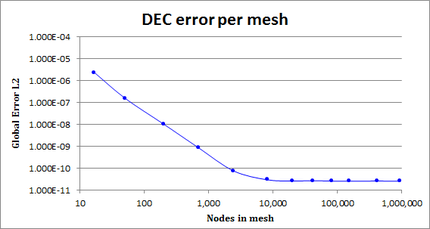
Table 4 shows some global error metrics for different meshes. Figure 21 shows the error evolution in ${\textstyle L^{2}}$ norm for this example.

Table 4. DEC errors in the second example

Mesh	Nodes	${\sum (u-u_{i})^{2} \over nodes}$	$L^{2}$ norm
1	17	1.5818e-04	2.3555e-06
2	51	2.5395e-05	1.5639e-07
3	201	3.3643e-06	1.0517e-08
4	713	5.1563e-07	8.3543e-10
5	2,455	8.9235e-08	7.6073e-11
6	8,180	3.1731e-08	2.9858e-11
7	20,016	2.0217e-08	2.6580e-11
8	42,306	1.4421e-08	2.7062e-11
9	82,722	9.8533e-09	2.6164e-11
10	156,274	7.1352e-09	2.5954e-11
11	420,013	4.4277e-09	2.6151e-11
12	935,016	2.9635e-09	2.6003e-11

Figure 21. DEC

error evolution in the second example

7.3 Third example: Heterogeneity and anisotropy

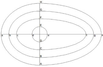
Let us solve the Poisson equation in a circle of radius on the following domain (Figure 22) with various material properties. The geometry of the domain is defined by segments of ellipses passing through the given points which have centers at the origin ${\textstyle (0,0)}$ .

Figure 22. Egg-like domain with different materials

Point	$x$	Point	$y$
a	-5	A	-4
b	-4	B	-3
c	-3	C	-2
d	-1	D	-1
e	1	E	1
f	6	F	2
g	7	G	3
h	8	H	4

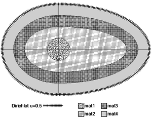
The Dirichlet boundary condition is ${\textstyle u=10}$ and material properties (anisotropic heat diffusion constants, material angles and source terms) are given according to Figure 23 and the table below.

Figure 23. Dirichlet condition

	$K_{x}$	$K_{y}$	Angle	$q$
Domain mat1	5	25	30	15
Domain mat2	25	5	0	5
Domain mat3	50	12	45	5
Domain mat4	10	35	0	5

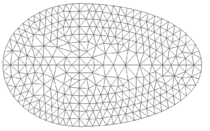
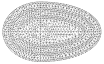
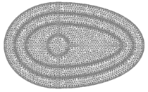
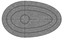
The meshes used in this example are shown in Figure 24.


(a)	(b)

(c)	(d)
Figure 24. Meshes for layered egg-like figure

The numerical results for the maximum temperature value ( ${\textstyle u(0,0)=10.2}$ ) are exemplified in Table 5 where a comparison with the Finite Element Method with linear interpolation functions (FEML) is also shown.

Table 5. Maximum temperature and Flux magnitude values in the numerical simulations of the third example

Mesh	Nodes	Elements	Max. Temp. Value		Max. Flux Magnitude
Mesh	Nodes	Elements	DEC	FEML	DEC	FEML
Figure 24(a)	342	616	2.79221	2.79854	18.41066	18.40573
Figure 24(b)	1,259	2,384	2.83929	2.84727	18.93838	18.91532
Figure 24(c)	4,467	8,668	2.85608	2.85717	19.13297	19.13193
Figure 24(d)	14,250	28,506	2.85994	2.86056	19.20982	19.20909
	20,493	40,316	2.86120	2.86177	19.23120	19.23457
	60,380	119,418	2.86219	2.86231	19.26655	19.26628
	142,702	283,162	2.86249	2.86256	19.28045	19.28028
	291,363	579,360	2.86263	2.86267	19.28727	19.28755
	495,607	986,724	2.86275	2.86269	19.29057	19.29081
	1,064,447	2,122,160	2.86272	2.86273	19.29385	19.29389
	2,106,077	4,202,536	2.86274	2.86274	19.29618	19.29615
	4,031,557	8,049,644	2.86275	2.86275	19.29763	19.29765

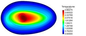
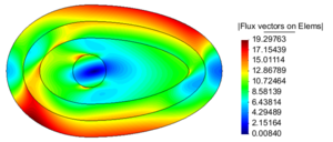
The temperature distribution and Flux magnitude fields for the finest mesh are shown in Figure 25.


(a) Contour fill of temperatures	(b) Contour till of flux vectors on elems
Figure 25. Temperature distribution and Flux magnitude fields for the finest mesh of the third example

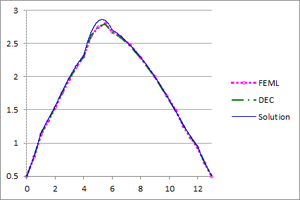
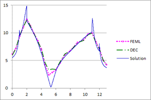
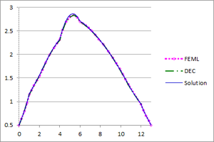
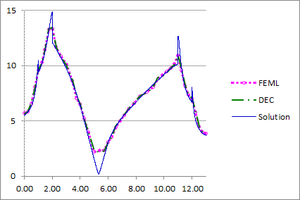
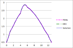
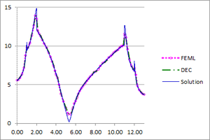
Figure 26 shows the graphs of the temperature and flux magnitude values along a diameter of the circle for different meshes of Figure 24.


(a)	(b)

(c)	(d)

(e)	(f)
Figure 26. Temperature and Flux magnitude graphs of the third example along a cross-section of the domain for different meshes: Mesh in Figure 24(a), a-Temperature, b-Flux; Mesh in Figure 24(b), c-Temperature, d-Flux; Mesh in Figure 24(c), e-Temperature, f-Flux

Table 6 shows some global error metrics for different meshes. Figure 27 shows the error evolution in ${\textstyle L^{2}}$ norm for this example.

Table 6. DEC errors in the third example

Mesh	Nodes	${\sum (u-u_{i})^{2} \over nodes}$	$L^{2}$ norm
1	342	9.3638e-04	2.7786e-02
2	1,259	1.5173e-04	3.2731e-03
3	4,467	2.2110e-05	2.2937e-04
4	14,250	3.7233e-06	1.9151e-05
5	20,492	2.2311e-06	9.5930e-06
6	60,380	4.3769e-07	8.7330e-07
7	142,702	1.1664e-07	1.3926e-07
8	291,369	3.9764e-08	3.3314e-08
9	497,378	1.6680e-08	1.0275e-08
10	1,067,171	3.9594e-09	1.2190e-09
11	2,106,248	9.6949e-10	1.4415e-10

Figure 27. DEC

evolution in the third example

Remark. As can be seen from the previous examples, DEC behaves well on coarse meshes. As expected, the results of DEC and FEML are identical for fine meshes. We would also like to point out the the computational costs of DEC and FEML are very similar since the local matrices are very similar in profile, or even identical in some cases.

8. Conclusions

DEC is a relatively recent discretization scheme for PDE's which takes into account the geometric and analytic features of the operators and the domains involved. The main contributions of this paper are the following:

We have made explicit the local formulation of DEC, i.e. on each triangle of the mesh. As is customary, the local pieces can be assembled, which facilitates the implementation of DEC by the interested reader. Furthermore, the profiles of the assembled DEC matrices are equal to those of assembled FEML matrices.
Guided by the local formulation, we have deduced a natural way to approximate the flux/gradient vector of a discretized function, which coincides with that of FEML. Such approximate flux vector automatically gives the discretized version of the anisotropic flux.
We have discretized the pullback operator on continuous 1-forms using Whitney interpolation forms and have found the discrete anisotropy operator for primal 1-forms.
We have deduced the local DEC formulation of the 2D anisotropic Poisson equation, and have proved that the DEC and FEML diffusion terms are identical, while the source terms are not – due to the different area-weight allocation for the nodes.
Local DEC allows a simple treatment of heterogeneous material properties assigned to subdomains (element by element), which eliminates the need of dealing with it through ad hoc modifications of the global discrete Hodge star operator matrix.

On the other hand we would like to point the following features:

The area weights assigned to the nodes of the mesh when solving the 2D anisotropic Poisson equation can even be negative (when a triangle has an inner angle greater that ${\textstyle 120^{\circ }}$ ), in stark contrast to the FEML formulation.

The computational cost of DEC is similar to that of FEML. While the numerical results of DEC and FEML on fine meshes are virtually identical, the DEC solutions are better than those of FEML on coarse meshes. Furthermore, DEC solutions display numerical convergence, as shown by the error measurements.

Our future work will include the DEC discretization of convective terms, and DEC on 2-dimensional simplicial surfaces in 3D. Preliminary results on both problems are promising and competitive with FEML.

Acknowledgements

The second named author was partially supported by a CONACyT grant, and would like to thank the International Centre for Numerical Methods in Engineering (CIMNE) and the University of Swansea for their hospitality. We gratefully acknowledge the support of NVIDIA Corporation with the donation of the Titan X Pascal GPU used for this research.

References

[1] Bossavit A. Mixed finite elements and the complex of Whitney forms. In J. Whiteman (ed.), The Mathematics of Finite Elements and Applications VI, pp. 137–144, Academic Press, 1988.

[2] Botello S., Moreles M.Z., Oñate E. Módulo de aplicaciones del método de los elementos finitos para resolver la ecuación de Poisson: MEFIPOISS. Aula CIMNE-CIMAT, Septiembre 2010.

[3] Cartan E. Sur certaines expressions différentielles et le problème de Pfaff. Annales Scientifiques de l'École Normale Supérieure, Série 3, Paris, Gauthier-Villars, Tome 16, pp. 239-332, 1899.

[4] Crane K., et al. Digital geometry processing with discrete exterior calculus. ACM SIGGRAPH 2013 Courses, pp. 1-126, July 2013.

[5] Dassios I., et al. A mathematical model for plasticity and damage: A discrete calculus formulation. Journal of Computational and Applied Mathematics, 312:27-38, 2017.

[6] Esqueda H., Herrera R., Botello S., Moreles M.A. A geometric description of discrete exterior calculus for general triangulations. Rev. Int. Métodos Numér. Cálc. Diseño Ing., 35(1), 2, 2019. https://www.scipedia.com/public/Herrera_et_al_2018b

[7] Griebel, M., Rieger C., Schier A. Upwind schemes for scalar advection-dominated problems in the Discrete Exterior Calculus. In Bothe D., Reusken A. (eds), Transport Processes at Fluidic Interfaces, Birkhäuser, Cham, 145-175, 2017.

[8] Hirani A.N. Discrete exterior calculus. Thesis, California Institute of Technology, 2003.

[9] Hirani A.N., Nakshatrala K.B., Chaudhry J.H. Numerical method for Darcy flow derived using discrete exterior calculus. International Journal for Computational Methods in Engineering Science and Mechanics, 16(3):151-169, 2015.

[10] Mohamed M.S., Hirani A.N., Samtaney R. Discrete exterior calculus discretization of incompressible Navier-Stokes equations over surface simplicial meshes. Journal of Computational Physics, 312: 175-191, 2016.

[11] Oñate E. 2D solids. Linear triangular and rectangular elements. In Structural Analysis with the Finite Element Method. Linear Statics, Volume 1: Basis and Solids, Chapter 4, pp. 117-157, CIMNE-Springer, Barcelona, 2009.

[12] Whitney H. Geometric integration theory. Princeton University Press, 1957.

[13] Zienkiewicz O.C., Taylor R.L., Zhu J.Z. Generalization of the finite element concepts. Galerkin-weighted residual and variational approaches. In The Finite Element Method Set (Sixth Edition), Butterworth-Heinemann, Oxford, Chapter 3, pp. 54-102, 2005.

Latest revision as of 15:49, 1 March 2021

Abstract

1. Introduction

2. Preliminaries on DEC from a local viewpoint

2.1 Boundary operator

2.2 Discrete derivative

2.3 Dual mesh

2.4 Discrete Hodge star

2.5 Continuous 1-forms

2.5.1 Pullback of a conitnuous 1-form

2.5.2 Discretization of continuous 1-forms

3. Pullback operator on primal 1-forms

4. Flux and anisotropy

4.1 The flux in local DEC

4.1.1 Comparison of DEC and FEML local fluxes

4.2 The anisotropic flux vector in local DEC

4.2.1 Geometric interpretation of the entries of $K^{DEC}$ 4.2.1 Geometric interpretation of the entries of K D E C {\displaystyle K^{DEC}}

5. Anisotropic Poisson equation in 2D

5.1 Local DEC discretization of the 2D anisotropic Poisson equation

5.2 Local FEML-Discretized 2D anisotropic Poisson equation

5.3 Comparison between local DEC and FEML discretizations

5.3.1 The diffusive term

5.3.2 The source term

6. Some remarks about DEC quantities

6.1 The discrete Hodge star quantities revisited

6.2 Area weights assigned to vertices

7. Numerical examples

7.1 First example: Heterogeneity

7.2 Second example: Anisotropy

7.3 Third example: Heterogeneity and anisotropy

8. Conclusions

Acknowledgements

References

Document information

Document Score

Share this document

Keywords

@@ Line 1,591: / Line 1,591: @@
 |  15.43724
 |}
 The temperature and flux-magnitude distribution fields are shown in  [[#img-14| Figure 14]].
@@ Line 1,647: / Line 1,648: @@
 <div class="center" style="font-size: 75%;">'''Table 2'''. DEC <math>L^2</math> errors in the first example</div>
-{|  class="floating_tableSCP wikitable" style="text-align: center; margin: 1em auto;min-width:50%;font-size:85%;"
+{| class="wikitable" style="margin: 1em auto 0.1em auto;border-collapse: collapse;font-size:85%;width:auto;"
-|- style="border-top: 2px solid;"
+|-style="text-align:center"
-| style="border-left: 2px solid;border-right: 2px solid;" |    '''Mesh'''
+! Mesh !! Nodes !!  <math>    \sum (u-u_i)^2 \over nodes    </math> !! <math>L^2</math> norm
-| style="border-left: 2px solid;border-right: 2px solid;" | '''Nodes'''
+|- style="text-align:center"
-| style="border-left: 2px solid;border-right: 2px solid;" | '''<math>    \sum (u-u_i)^2 \over nodes    </math>'''
+|    1
-| style="border-left: 2px solid;border-right: 2px solid;" | '''<math>L^2</math> norm'''
+|  49
-|- style="border-top: 2px solid;"
+|  1.0537e-02
-| style="border-left: 2px solid;border-right: 1px solid;" |    1
+|  1.4438e-01
-| style="border-left: 1px solid;border-right: 1px solid;" | 49
+|- style="text-align:center"
-| style="border-left: 1px solid;border-right: 1px solid;" | 1.0537e-02
+|    2
-| style="border-left: 1px solid;border-right: 2px solid;" | 1.4438e-01
+|  98
-|-
+|  4.2447e-03
-| style="border-left: 2px solid;border-right: 1px solid;" |    2
+|  4.8558e-02
-| style="border-left: 1px solid;border-right: 1px solid;" | 98
+|- style="text-align:center"
-| style="border-left: 1px solid;border-right: 1px solid;" | 4.2447e-03
+|    3
-| style="border-left: 1px solid;border-right: 2px solid;" | 4.8558e-02
+|  258
-|-
+|  6.9781e-04
-| style="border-left: 2px solid;border-right: 1px solid;" |    3
+|  3.0390e-03
-| style="border-left: 1px solid;border-right: 1px solid;" | 258
+|- style="text-align:center"
-| style="border-left: 1px solid;border-right: 1px solid;" | 6.9781e-04
+|    4
-| style="border-left: 1px solid;border-right: 2px solid;" | 3.0390e-03
+|  1,010
-|-
+|  8.8386e-05
-| style="border-left: 2px solid;border-right: 1px solid;" |    4
+|  1.4877e-04
-| style="border-left: 1px solid;border-right: 1px solid;" | 1,010
+|- style="text-align:center"
-| style="border-left: 1px solid;border-right: 1px solid;" | 8.8386e-05
+|    5
-| style="border-left: 1px solid;border-right: 2px solid;" | 1.4877e-04
+|  3,813
-|-
+|  1.0736e-05
-| style="border-left: 2px solid;border-right: 1px solid;" |    5
+|  7.7369e-06
-| style="border-left: 1px solid;border-right: 1px solid;" | 3,813
+|- style="text-align:center"
-| style="border-left: 1px solid;border-right: 1px solid;" | 1.0736e-05
+|    6
-| style="border-left: 1px solid;border-right: 2px solid;" | 7.7369e-06
+|  13,911
-|-
+|  1.4422e-06
-| style="border-left: 2px solid;border-right: 1px solid;" |    6
+|  4.9791e-07
-| style="border-left: 1px solid;border-right: 1px solid;" | 13,911
+|- style="text-align:center"
-| style="border-left: 1px solid;border-right: 1px solid;" | 1.4422e-06
+|    7
-| style="border-left: 1px solid;border-right: 2px solid;" | 4.9791e-07
+|  50,950
-|-
+|  1.7582e-07
-| style="border-left: 2px solid;border-right: 1px solid;" |    7
+|  2.9608e-08
-| style="border-left: 1px solid;border-right: 1px solid;" | 50,950
+|- style="text-align:center"
-| style="border-left: 1px solid;border-right: 1px solid;" | 1.7582e-07
+|    8
-| style="border-left: 1px solid;border-right: 2px solid;" | 2.9608e-08
+|  135,518
-|-
+|  3.2621e-08
-| style="border-left: 2px solid;border-right: 1px solid;" |    8
+|  2.9233e-09
-| style="border-left: 1px solid;border-right: 1px solid;" | 135,518
+|- style="text-align:center"
-| style="border-left: 1px solid;border-right: 1px solid;" | 3.2621e-08
+|    9
-| style="border-left: 1px solid;border-right: 2px solid;" | 2.9233e-09
+|  298,299
-|-
+|  7.3566e-09
-| style="border-left: 2px solid;border-right: 1px solid;" |    9
+|  3.3610e-10
-| style="border-left: 1px solid;border-right: 1px solid;" | 298,299
+|- style="text-align:center"
-| style="border-left: 1px solid;border-right: 1px solid;" | 7.3566e-09
+|    10
-| style="border-left: 1px solid;border-right: 2px solid;" | 3.3610e-10
+|  603,440
-|- style="border-top: 1px solid;border-bottom: 2px solid;"
+|  1.8577e-09
-| style="border-left: 2px solid;border-right: 1px solid;" |    10
+|  4.9496e-11
-| style="border-left: 1px solid;border-right: 1px solid;" | 603,440
-| style="border-left: 1px solid;border-right: 1px solid;" | 1.8577e-09
-| style="border-left: 1px solid;border-right: 2px solid;" | 4.9496e-11
 |}
@@ Line 1,768: / Line 1,766: @@
 <div style="text-align: center; font-size: 75%; ">'''Table 3'''. Temperature value at the point (0,0) and Flux magnitude value at the point (-1, 0) of the numerical simulations for the second example</div>
-{|  class="floating_tableSCP wikitable" style="text-align: center; margin: 1em auto;min-width:50%;font-size:85%;"
+{| class="wikitable" style="margin: 1em auto 0.1em auto;border-collapse: collapse;font-size:85%;width:auto;"
-|- style="border-top: 2px solid;border-bottom: 2px solid;"
+|-style="text-align:center"
-| rowspan='2' style="border-left: 2px solid;border-right: 2px solid;" | Mesh
+!  rowspan='2'  | Mesh !!  rowspan='2' |  Nodes !!  rowspan='2' | Elements !!  colspan='2' | Temp. Value at <math>(0,0)</math> !!  colspan='2'  | Flux Magnitude at <math>(-1,0)</math>
-| rowspan='2' style="border-left: 2px solid;border-right: 2px solid;" | Nodes
+|-style="text-align:center"
-| rowspan='2' style="border-left: 2px solid;border-right: 2px solid;" | Elements
+! DEC  !!   FEML !!   DEC  !!  FEML
-| colspan='2' style="border-right: 2px solid;border-left: 2px solid;border-right: 2px solid;" | Temp. Value at <math>(0,0)</math>
+|- style="text-align:center"
-| colspan='2' style="border-right: 2px solid;border-left: 2px solid;border-right: 2px solid;" | Flux Magnitude at <math>(-1,0)</math>
+|  [[#img-18|Figure 18]](a)
-|-style="border-top: 2px solid;border-bottom: 2px solid;"
+|  17
-| style="border-left: 2px solid;border-right: 1px solid;" | DEC
+|  20
-| style="border-left: 1px solid;border-right: 1px solid;" | FEML
+|  10.20014
-| style="border-left: 1px solid;border-right: 1px solid;" | DEC
+|  10.19002
-| style="border-left: 1px solid;border-right: 2px solid;" | FEML
+|  0.42133
-|-
+|  0.43865
-| style="border-left: 2px solid;border-right: 1px solid;" |  [[#img-18|Figure 18]](a)
+|-style="text-align:center"
-| style="border-left: 1px solid;border-right: 1px solid;" | 17
+| [[#img-18|Figure 18]](b)
-| style="border-left: 1px solid;border-right: 1px solid;" | 20
+|  41
-| style="border-left: 1px solid;border-right: 1px solid;" | 10.20014
+|  56
-| style="border-left: 1px solid;border-right: 1px solid;" | 10.19002
+|  10.20007
-| style="border-left: 1px solid;border-right: 1px solid;" | 0.42133
+|  10.19678
-| style="border-left: 1px solid;border-right: 2px solid;" | 0.43865
+|  0.48544
-|-
+|  0.49387
-| style="border-left: 2px solid;border-right: 1px solid;" | [[#img-18|Figure 18]](b)
+|-style="text-align:center"
-| style="border-left: 1px solid;border-right: 1px solid;" | 41
+| [[#img-18|Figure 18]](c)
-| style="border-left: 1px solid;border-right: 1px solid;" | 56
+|  201
-| style="border-left: 1px solid;border-right: 1px solid;" | 10.20007
+|  344
-| style="border-left: 1px solid;border-right: 1px solid;" | 10.19678
+|  10.20012
-| style="border-left: 1px solid;border-right: 1px solid;" | 0.48544
+|  10.20158
-| style="border-left: 1px solid;border-right: 2px solid;" | 0.49387
+|  0.52470
-|-
+|  0.52428
-| style="border-left: 2px solid;border-right: 1px solid;" | [[#img-18|Figure 18]](c)
+|-style="text-align:center"
-| style="border-left: 1px solid;border-right: 1px solid;" | 201
+| [[#img-18|Figure 18]](d)
-| style="border-left: 1px solid;border-right: 1px solid;" | 344
+|  713
-| style="border-left: 1px solid;border-right: 1px solid;" | 10.20012
+|  1304
-| style="border-left: 1px solid;border-right: 1px solid;" | 10.20158
+|  10.20000
-| style="border-left: 1px solid;border-right: 1px solid;" | 0.52470
+|  10.19969
-| style="border-left: 1px solid;border-right: 2px solid;" | 0.52428
+|  0.54143
-|-
+|  0.54224
-| style="border-left: 2px solid;border-right: 1px solid;" | [[#img-18|Figure 18]](d)
+|-style="text-align:center"
-| style="border-left: 1px solid;border-right: 1px solid;" | 713
+|  [[#img-18|Figure 18]](e)
-| style="border-left: 1px solid;border-right: 1px solid;" | 1304
+|  2455
-| style="border-left: 1px solid;border-right: 1px solid;" | 10.20000
+|  4660
-| style="border-left: 1px solid;border-right: 1px solid;" | 10.19969
+|  10.20000
-| style="border-left: 1px solid;border-right: 1px solid;" | 0.54143
+|  10.19990
-| style="border-left: 1px solid;border-right: 2px solid;" | 0.54224
+|  0.54971
-|-
+|  0.55138
-| style="border-left: 2px solid;border-right: 1px solid;" |  [[#img-18|Figure 18]](e)
+|-style="text-align:center"
-| style="border-left: 1px solid;border-right: 1px solid;" | 2455
+|  [[#img-18|Figure 18]](f)
-| style="border-left: 1px solid;border-right: 1px solid;" | 4660
+|  8180
-| style="border-left: 1px solid;border-right: 1px solid;" | 10.20000
+|  15862
-| style="border-left: 1px solid;border-right: 1px solid;" | 10.19990
+|  10.20000
-| style="border-left: 1px solid;border-right: 1px solid;" | 0.54971
+|  10.20002
-| style="border-left: 1px solid;border-right: 2px solid;" | 0.55138
+|  0.55326
-|-
+|  0.55409
-| style="border-left: 2px solid;border-right: 1px solid;" |  [[#img-18|Figure 18]](f)
+|-style="text-align:center"
-| style="border-left: 1px solid;border-right: 1px solid;" | 8180
+|
-| style="border-left: 1px solid;border-right: 1px solid;" | 15862
+|  20016
-| style="border-left: 1px solid;border-right: 1px solid;" | 10.20000
+|  39198
-| style="border-left: 1px solid;border-right: 1px solid;" | 10.20002
+|  10.20000
-| style="border-left: 1px solid;border-right: 1px solid;" | 0.55326
+|  10.19999
-| style="border-left: 1px solid;border-right: 2px solid;" | 0.55409
+|  0.55470
-|-
+|  0.55520
-| style="border-left: 2px solid;border-right: 1px solid;" |
+|- style="text-align:center"
-| style="border-left: 1px solid;border-right: 1px solid;" | 20016
+|
-| style="border-left: 1px solid;border-right: 1px solid;" | 39198
+|  42306
-| style="border-left: 1px solid;border-right: 1px solid;" | 10.20000
+|  83362
-| style="border-left: 1px solid;border-right: 1px solid;" | 10.19999
+|  10.20000
-| style="border-left: 1px solid;border-right: 1px solid;" | 0.55470
+|  10.20000
-| style="border-left: 1px solid;border-right: 2px solid;" | 0.55520
+|  0.55540
-|- style="border-bottom: 2px solid;"
+|  0.55572
-| style="border-left: 2px solid;border-right: 1px solid;" |
-| style="border-left: 1px solid;border-right: 1px solid;" | 42306
-| style="border-left: 1px solid;border-right: 1px solid;" | 83362
-| style="border-left: 1px solid;border-right: 1px solid;" | 10.20000
-| style="border-left: 1px solid;border-right: 1px solid;" | 10.20000
-| style="border-left: 1px solid;border-right: 1px solid;" | 0.55540
-| style="border-left: 1px solid;border-right: 2px solid;" | 0.55572
 |}
@@ Line 1,902: / Line 1,893: @@
 <div class="center" style="font-size: 75%;">'''Table 4'''. DEC errors in the second example</div>
-{|  class="floating_tableSCP wikitable" style="text-align: center; margin: 1em auto;min-width:50%;font-size:85%;"
+{| class="wikitable" style="margin: 1em auto 0.1em auto;border-collapse: collapse;font-size:85%;width:auto;"
-|- style="border-top: 2px solid;"
+|-style="text-align:center"
-| style="border-left: 2px solid;border-right: 2px solid;" |    '''Mesh'''
+! Mesh !! Nodes !!  <math>    \sum (u-u_i)^2 \over nodes    </math> !! <math>L^2</math> norm
-| style="border-left: 2px solid;border-right: 2px solid;" | '''Nodes'''
+|- style="text-align:center"
-| style="border-left: 2px solid;border-right: 2px solid;" | '''<math>    \sum (u-u_i)^2 \over nodes    </math>'''
+|     1
-| style="border-left: 2px solid;border-right: 2px solid;" | '''<math>L^2</math> norm'''
+|  17
-|- style="border-top: 2px solid;"
+|  1.5818e-04
-| style="border-left: 2px solid;border-right: 1px solid;" |     1
+|  2.3555e-06
-| style="border-left: 1px solid;border-right: 1px solid;" | 17
+|- style="text-align:center"
-| style="border-left: 1px solid;border-right: 1px solid;" | 1.5818e-04
+|     2
-| style="border-left: 1px solid;border-right: 2px solid;" | 2.3555e-06
+|  51
-|- style="border-top: 1px solid;"
+|  2.5395e-05
-| style="border-left: 2px solid;border-right: 1px solid;" |     2
+|  1.5639e-07
-| style="border-left: 1px solid;border-right: 1px solid;" | 51
+|- style="text-align:center"
-| style="border-left: 1px solid;border-right: 1px solid;" | 2.5395e-05
+|     3
-| style="border-left: 1px solid;border-right: 2px solid;" | 1.5639e-07
+|  201
-|- style="border-top: 1px solid;"
+|  3.3643e-06
-| style="border-left: 2px solid;border-right: 1px solid;" |     3
+|  1.0517e-08
-| style="border-left: 1px solid;border-right: 1px solid;" | 201
+|- style="text-align:center"
-| style="border-left: 1px solid;border-right: 1px solid;" | 3.3643e-06
+|     4
-| style="border-left: 1px solid;border-right: 2px solid;" | 1.0517e-08
+|  713
-|- style="border-top: 1px solid;"
+|  5.1563e-07
-| style="border-left: 2px solid;border-right: 1px solid;" |     4
+|  8.3543e-10
-| style="border-left: 1px solid;border-right: 1px solid;" | 713
+|- style="text-align:center"
-| style="border-left: 1px solid;border-right: 1px solid;" | 5.1563e-07
+|     5
-| style="border-left: 1px solid;border-right: 2px solid;" | 8.3543e-10
+|  2,455
-|- style="border-top: 1px solid;"
+|  8.9235e-08
-| style="border-left: 2px solid;border-right: 1px solid;" |     5
+|  7.6073e-11
-| style="border-left: 1px solid;border-right: 1px solid;" | 2,455
+|- style="text-align:center"
-| style="border-left: 1px solid;border-right: 1px solid;" | 8.9235e-08
+|     6
-| style="border-left: 1px solid;border-right: 2px solid;" | 7.6073e-11
+|  8,180
-|- style="border-top: 1px solid;"
+|  3.1731e-08
-| style="border-left: 2px solid;border-right: 1px solid;" |     6
+|  2.9858e-11
-| style="border-left: 1px solid;border-right: 1px solid;" | 8,180
+|- style="text-align:center"
-| style="border-left: 1px solid;border-right: 1px solid;" | 3.1731e-08
+|     7
-| style="border-left: 1px solid;border-right: 2px solid;" | 2.9858e-11
+|  20,016
-|- style="border-top: 1px solid;"
+|  2.0217e-08
-| style="border-left: 2px solid;border-right: 1px solid;" |     7
+|  2.6580e-11
-| style="border-left: 1px solid;border-right: 1px solid;" | 20,016
+|- style="text-align:center"
-| style="border-left: 1px solid;border-right: 1px solid;" | 2.0217e-08
+|     8
-| style="border-left: 1px solid;border-right: 2px solid;" | 2.6580e-11
+|  42,306
-|- style="border-top: 1px solid;"
+|  1.4421e-08
-| style="border-left: 2px solid;border-right: 1px solid;" |     8
+|  2.7062e-11
-| style="border-left: 1px solid;border-right: 1px solid;" | 42,306
+|- style="text-align:center"
-| style="border-left: 1px solid;border-right: 1px solid;" | 1.4421e-08
+|     9
-| style="border-left: 1px solid;border-right: 2px solid;" | 2.7062e-11
+|  82,722
-|- style="border-top: 1px solid;"
+|  9.8533e-09
-| style="border-left: 2px solid;border-right: 1px solid;" |     9
+|  2.6164e-11
-| style="border-left: 1px solid;border-right: 1px solid;" | 82,722
+|- style="text-align:center"
-| style="border-left: 1px solid;border-right: 1px solid;" | 9.8533e-09
+|     10
-| style="border-left: 1px solid;border-right: 2px solid;" | 2.6164e-11
+|  156,274
-|- style="border-top: 1px solid;"
+|  7.1352e-09
-| style="border-left: 2px solid;border-right: 1px solid;" |     10
+|  2.5954e-11
-| style="border-left: 1px solid;border-right: 1px solid;" | 156,274
+|- style="text-align:center"
-| style="border-left: 1px solid;border-right: 1px solid;" | 7.1352e-09
+|     11
-| style="border-left: 1px solid;border-right: 2px solid;" | 2.5954e-11
+|  420,013
-|- style="border-top: 1px solid;"
+|  4.4277e-09
-| style="border-left: 2px solid;border-right: 1px solid;" |     11
+|  2.6151e-11
-| style="border-left: 1px solid;border-right: 1px solid;" | 420,013
+|- style="text-align:center"
-| style="border-left: 1px solid;border-right: 1px solid;" | 4.4277e-09
+|     12
-| style="border-left: 1px solid;border-right: 2px solid;" | 2.6151e-11
+|  935,016
-|- style="border-top: 1px solid;border-bottom: 2px solid;"
+|  2.9635e-09
-| style="border-left: 2px solid;border-right: 1px solid;" |     12
+|  2.6003e-11
-| style="border-left: 1px solid;border-right: 1px solid;" | 935,016
-| style="border-left: 1px solid;border-right: 1px solid;" | 2.9635e-09
-| style="border-left: 1px solid;border-right: 2px solid;" | 2.6003e-11
 |}
@@ Line 1,992: / Line 1,980: @@
-{|  class="floating_tableSCP wikitable" style="text-align: center; margin: 1em auto;min-width:40%;font-size:85%;"
+{| class="wikitable" style="margin: 1em auto 0.1em auto;border-collapse: collapse;font-size:85%;width:auto;"
-|- style="border-top: 2px solid;"
+|-style="text-align:center"
-| style="border-left: 2px solid;border-right: 2px solid;" |    Point
+!   Point !!  <math>x</math> !!  <math>y</math> !!  Point !!  <math>x</math> !! <math>y</math>
-| style="border-left: 2px solid;border-right: 2px solid;" | <math>x</math>
+|- style="text-align:center"
-| style="border-left: 2px solid;border-right: 2px solid;" | <math>y</math>
+|    a
-| style="border-left: 2px solid;border-right: 2px solid;" | Point
+|  -5
-| style="border-left: 2px solid;border-right: 2px solid;" | <math>x</math>
+|  0
-| style="border-left: 2px solid;border-right: 2px solid;" | <math>y</math>
+|  A
-|- style="border-top: 2px solid;"
+|  0
-| style="border-left: 2px solid;border-right: 1px solid;" |    a
+|  -4
-| style="border-left: 1px solid;border-right: 1px solid;" | -5
+|-style="text-align:center"
-| style="border-left: 1px solid;border-right: 1px solid;" | 0
+| b
-| style="border-left: 1px solid;border-right: 1px solid;" | A
+|  -4
-| style="border-left: 1px solid;border-right: 1px solid;" | 0
+|  0
-| style="border-left: 1px solid;border-right: 2px solid;" | -4
+|  B
-|-
+|  0
-| style="border-left: 2px solid;border-right: 1px solid;" | b
+|  -3
-| style="border-left: 1px solid;border-right: 1px solid;" | -4
+|-style="text-align:center"
-| style="border-left: 1px solid;border-right: 1px solid;" | 0
+| c
-| style="border-left: 1px solid;border-right: 1px solid;" | B
+|  -3
-| style="border-left: 1px solid;border-right: 1px solid;" | 0
+|  0
-| style="border-left: 1px solid;border-right: 2px solid;" | -3
+|  C
-|-
+|  0
-| style="border-left: 2px solid;border-right: 1px solid;" | c
+|  -2
-| style="border-left: 1px solid;border-right: 1px solid;" | -3
+|-style="text-align:center"
-| style="border-left: 1px solid;border-right: 1px solid;" | 0
+| d
-| style="border-left: 1px solid;border-right: 1px solid;" | C
+|  -1
-| style="border-left: 1px solid;border-right: 1px solid;" | 0
+|  0
-| style="border-left: 1px solid;border-right: 2px solid;" | -2
+|  D
-|-
+|  0
-| style="border-left: 2px solid;border-right: 1px solid;" | d
+|  -1
-| style="border-left: 1px solid;border-right: 1px solid;" | -1
+|-style="text-align:center"
-| style="border-left: 1px solid;border-right: 1px solid;" | 0
+| e
-| style="border-left: 1px solid;border-right: 1px solid;" | D
+|  1
-| style="border-left: 1px solid;border-right: 1px solid;" | 0
+|  0
-| style="border-left: 1px solid;border-right: 2px solid;" | -1
+|  E
-|-
+|  0
-| style="border-left: 2px solid;border-right: 1px solid;" | e
+|  1
-| style="border-left: 1px solid;border-right: 1px solid;" | 1
+|-style="text-align:center"
-| style="border-left: 1px solid;border-right: 1px solid;" | 0
+| f
-| style="border-left: 1px solid;border-right: 1px solid;" | E
+|  6
-| style="border-left: 1px solid;border-right: 1px solid;" | 0
+|  0
-| style="border-left: 1px solid;border-right: 2px solid;" | 1
+|  F
-|-
+|  0
-| style="border-left: 2px solid;border-right: 1px solid;" | f
+|  2
-| style="border-left: 1px solid;border-right: 1px solid;" | 6
+|-style="text-align:center"
-| style="border-left: 1px solid;border-right: 1px solid;" | 0
+| g
-| style="border-left: 1px solid;border-right: 1px solid;" | F
+|  7
-| style="border-left: 1px solid;border-right: 1px solid;" | 0
+|  0
-| style="border-left: 1px solid;border-right: 2px solid;" | 2
+|  G
-|-
+|  0
-| style="border-left: 2px solid;border-right: 1px solid;" | g
+|  3
-| style="border-left: 1px solid;border-right: 1px solid;" | 7
+|- style="text-align:center"
-| style="border-left: 1px solid;border-right: 1px solid;" | 0
+| h
-| style="border-left: 1px solid;border-right: 1px solid;" | G
+|  8
-| style="border-left: 1px solid;border-right: 1px solid;" | 0
+|  0
-| style="border-left: 1px solid;border-right: 2px solid;" | 3
+|  H
-|- style="border-bottom: 2px solid;"
+|  0
-| style="border-left: 2px solid;border-right: 1px solid;" | h
+|  4
-| style="border-left: 1px solid;border-right: 1px solid;" | 8
-| style="border-left: 1px solid;border-right: 1px solid;" | 0
-| style="border-left: 1px solid;border-right: 1px solid;" | H
-| style="border-left: 1px solid;border-right: 1px solid;" | 0
-| style="border-left: 1px solid;border-right: 2px solid;" | 4
 |}
@@ Line 2,070: / Line 2,053: @@
-{|  class="floating_tableSCP wikitable" style="text-align: center; margin: 1em auto;min-width:40%;font-size:85%;"
+{| class="wikitable" style="margin: 1em auto 0.1em auto;border-collapse: collapse;font-size:85%;width:auto;"
-|- style="border-top: 2px solid;"
+|-style="text-align:center"
-| style="text-align: left;border-left: 2px solid;border-right: 2px solid;" |
+! !!  <math>K_x</math> !! <math>K_y</math> !! Angle !!  <math>q</math>
-| style="border-left: 2px solid;border-right: 2px solid;" | <math>K_x</math>
+|- style="text-align:center"
-| style="border-left: 2px solid;border-right: 2px solid;" | <math>K_y</math>
+|  Domain mat1
-| style="border-left: 2px solid;border-right: 2px solid;" | Angle
+|  5
-| style="border-left: 2px solid;border-right: 2px solid;" | <math>q</math>
+|  25
-|- style="border-top: 2px solid;"
+| 30
-| style="text-align: left;border-left: 2px solid;border-right: 1px solid;" |     Domain mat1
+|  15
-| style="border-left: 1px solid;border-right: 1px solid;" | 5
+|- style="text-align:center"
-| style="border-left: 1px solid;border-right: 1px solid;" | 25
+| style="text-align: left;" |     Domain mat2
-| style="border-left: 1px solid;border-right: 1px solid;" | 30
+|  25
-| style="border-left: 1px solid;border-right: 2px solid;" | 15
+|  5
-|- style="border-top: 1px solid;"
+|  0
-| style="text-align: left;border-left: 2px solid;border-right: 1px solid;" |     Domain mat2
+|  5
-| style="border-left: 1px solid;border-right: 1px solid;" | 25
+|- style="text-align:center"
-| style="border-left: 1px solid;border-right: 1px solid;" | 5
+| style="text-align: left;" |     Domain mat3
-| style="border-left: 1px solid;border-right: 1px solid;" | 0
+|  50
-| style="border-left: 1px solid;border-right: 2px solid;" | 5
+|  12
-|- style="border-top: 1px solid;"
+|  45
-| style="text-align: left;border-left: 2px solid;border-right: 1px solid;" |     Domain mat3
+|  5
-| style="border-left: 1px solid;border-right: 1px solid;" | 50
+|- style="text-align:center"
-| style="border-left: 1px solid;border-right: 1px solid;" | 12
+| style="text-align: left;" |     Domain mat4
-| style="border-left: 1px solid;border-right: 1px solid;" | 45
+|  10
-| style="border-left: 1px solid;border-right: 2px solid;" | 5
+| 35
-|- style="border-top: 1px solid;border-bottom: 2px solid;"
+| 0
-| style="text-align: left;border-left: 2px solid;border-right: 1px solid;" |     Domain mat4
+|  5
-| style="border-left: 1px solid;border-right: 1px solid;" | 10
-| style="border-left: 1px solid;border-right: 1px solid;" | 35
-| style="border-left: 1px solid;border-right: 1px solid;" | 0
-| style="border-left: 1px solid;border-right: 2px solid;" | 5
 |}
@@ Line 2,134: / Line 2,113: @@
 <div style="text-align: center; font-size: 75%; ">'''Table 5'''. Maximum temperature and Flux magnitude values in the numerical simulations of the third example</div>
-{|  class="floating_tableSCP wikitable" style="text-align: center; margin: 1em auto;min-width:50%;font-size:85%;"
+{| class="wikitable" style="margin: 1em auto 0.1em auto;border-collapse: collapse;font-size:85%;width:auto;"
-|- style="border-top: 2px solid;"
+|-style="text-align:center"
-| rowspan='2' style="border-left: 2px solid;border-right: 2px solid;" | Mesh
+! rowspan='2' | Mesh !!  rowspan='2' | Nodes !!  rowspan='2'  | Elements !!  colspan='2' | Max. Temp. Value !! colspan='2'  | Max. Flux Magnitude
-| rowspan='2' style="border-left: 2px solid;border-right: 2px solid;" | Nodes
+|-style="text-align:center"
-| rowspan='2' style="border-left: 2px solid;border-right: 2px solid;" | Elements
+!  DEC  !!  FEML !!  DEC  !!  FEML
-| colspan='2' style="border-right: 2px solid;border-left: 2px solid;border-right: 2px solid;" | Max. Temp. Value
+|- style="text-align:center"
-| colspan='2' style="border-right: 2px solid;border-left: 2px solid;border-right: 2px solid;" | Max. Flux Magnitude
+| [[#img-24|Figure 24]](a)
-|-style="border-top: 2px solid;"
+|  342
-| style="border-left: 2px solid;border-right: 2px solid;" | DEC
+|  616
-| style="border-left: 2px solid;border-right: 2px solid;" | FEML
+|  2.79221
-| style="border-left: 2px solid;border-right: 2px solid;" | DEC
+|  2.79854
-| style="border-left: 2px solid;border-right: 2px solid;" | FEML
+|  18.41066
-|- style="border-top: 2px solid;"
+|  18.40573
-| style="border-left: 2px solid;border-right: 1px solid;" |     [[#img-24|Figure 24]](a)
+|-style="text-align:center"
-| style="border-left: 1px solid;border-right: 1px solid;" | 342
+|  [[#img-24|Figure 24]](b)
-| style="border-left: 1px solid;border-right: 1px solid;" | 616
+|  1,259
-| style="border-left: 1px solid;border-right: 1px solid;" | 2.79221
+|  2,384
-| style="border-left: 1px solid;border-right: 1px solid;" | 2.79854
+|  2.83929
-| style="border-left: 1px solid;border-right: 1px solid;" | 18.41066
+|  2.84727
-| style="border-left: 1px solid;border-right: 2px solid;" | 18.40573
+|  18.93838
-|-
+|  18.91532
-| style="border-left: 2px solid;border-right: 1px solid;" |  [[#img-24|Figure 24]](b)
+|-style="text-align:center"
-| style="border-left: 1px solid;border-right: 1px solid;" | 1,259
+|  [[#img-24|Figure 24]](c)
-| style="border-left: 1px solid;border-right: 1px solid;" | 2,384
+|  4,467
-| style="border-left: 1px solid;border-right: 1px solid;" | 2.83929
+|  8,668
-| style="border-left: 1px solid;border-right: 1px solid;" | 2.84727
+|  2.85608
-| style="border-left: 1px solid;border-right: 1px solid;" | 18.93838
+|  2.85717
-| style="border-left: 1px solid;border-right: 2px solid;" | 18.91532
+|  19.13297
-|-
+|  19.13193
-| style="border-left: 2px solid;border-right: 1px solid;" |  [[#img-24|Figure 24]](c)
+|-style="text-align:center"
-| style="border-left: 1px solid;border-right: 1px solid;" | 4,467
+|  [[#img-24|Figure 24]](d)
-| style="border-left: 1px solid;border-right: 1px solid;" | 8,668
+|  14,250
-| style="border-left: 1px solid;border-right: 1px solid;" | 2.85608
+|  28,506
-| style="border-left: 1px solid;border-right: 1px solid;" | 2.85717
+|  2.85994
-| style="border-left: 1px solid;border-right: 1px solid;" | 19.13297
+|  2.86056
-| style="border-left: 1px solid;border-right: 2px solid;" | 19.13193
+|  19.20982
-|-
+|  19.20909
-| style="border-left: 2px solid;border-right: 1px solid;" |  [[#img-24|Figure 24]](d)
+|-style="text-align:center"
-| style="border-left: 1px solid;border-right: 1px solid;" | 14,250
+|
-| style="border-left: 1px solid;border-right: 1px solid;" | 28,506
+|  20,493
-| style="border-left: 1px solid;border-right: 1px solid;" | 2.85994
+|  40,316
-| style="border-left: 1px solid;border-right: 1px solid;" | 2.86056
+|  2.86120
-| style="border-left: 1px solid;border-right: 1px solid;" | 19.20982
+|  2.86177
-| style="border-left: 1px solid;border-right: 2px solid;" | 19.20909
+|  19.23120
-|-
+|  19.23457
-| style="border-left: 2px solid;border-right: 1px solid;" |
+|-style="text-align:center"
-| style="border-left: 1px solid;border-right: 1px solid;" | 20,493
+|
-| style="border-left: 1px solid;border-right: 1px solid;" | 40,316
+|  60,380
-| style="border-left: 1px solid;border-right: 1px solid;" | 2.86120
+|  119,418
-| style="border-left: 1px solid;border-right: 1px solid;" | 2.86177
+|  2.86219
-| style="border-left: 1px solid;border-right: 1px solid;" | 19.23120
+|  2.86231
-| style="border-left: 1px solid;border-right: 2px solid;" | 19.23457
+|  19.26655
-|-
+|  19.26628
-| style="border-left: 2px solid;border-right: 1px solid;" |
+|-style="text-align:center"
-| style="border-left: 1px solid;border-right: 1px solid;" | 60,380
+|
-| style="border-left: 1px solid;border-right: 1px solid;" | 119,418
+|  142,702
-| style="border-left: 1px solid;border-right: 1px solid;" | 2.86219
+|  283,162
-| style="border-left: 1px solid;border-right: 1px solid;" | 2.86231
+|  2.86249
-| style="border-left: 1px solid;border-right: 1px solid;" | 19.26655
+|  2.86256
-| style="border-left: 1px solid;border-right: 2px solid;" | 19.26628
+|  19.28045
-|-
+|  19.28028
-| style="border-left: 2px solid;border-right: 1px solid;" |
+|-style="text-align:center"
-| style="border-left: 1px solid;border-right: 1px solid;" | 142,702
+|
-| style="border-left: 1px solid;border-right: 1px solid;" | 283,162
+|  291,363
-| style="border-left: 1px solid;border-right: 1px solid;" | 2.86249
+|  579,360
-| style="border-left: 1px solid;border-right: 1px solid;" | 2.86256
+|  2.86263
-| style="border-left: 1px solid;border-right: 1px solid;" | 19.28045
+|  2.86267
-| style="border-left: 1px solid;border-right: 2px solid;" | 19.28028
+|  19.28727
-|-
+|  19.28755
-| style="border-left: 2px solid;border-right: 1px solid;" |
+|-style="text-align:center"
-| style="border-left: 1px solid;border-right: 1px solid;" | 291,363
+|
-| style="border-left: 1px solid;border-right: 1px solid;" | 579,360
+|  495,607
-| style="border-left: 1px solid;border-right: 1px solid;" | 2.86263
+|  986,724
-| style="border-left: 1px solid;border-right: 1px solid;" | 2.86267
+|  2.86275
-| style="border-left: 1px solid;border-right: 1px solid;" | 19.28727
+|  2.86269
-| style="border-left: 1px solid;border-right: 2px solid;" | 19.28755
+|  19.29057
-|-
+|  19.29081
-| style="border-left: 2px solid;border-right: 1px solid;" |
-| style="border-left: 1px solid;border-right: 1px solid;" | 495,607
-| style="border-left: 1px solid;border-right: 1px solid;" | 986,724
-| style="border-left: 1px solid;border-right: 1px solid;" | 2.86275
-| style="border-left: 1px solid;border-right: 1px solid;" | 2.86269
-| style="border-left: 1px solid;border-right: 1px solid;" | 19.29057
-| style="border-left: 1px solid;border-right: 2px solid;" | 19.29081
-|-
-| style="border-left: 2px solid;border-right: 1px solid;" |
-| style="border-left: 1px solid;border-right: 1px solid;" | 1,064,447
-| style="border-left: 1px solid;border-right: 1px solid;" | 2,122,160
-| style="border-left: 1px solid;border-right: 1px solid;" | 2.86272
-| style="border-left: 1px solid;border-right: 1px solid;" | 2.86273
-| style="border-left: 1px solid;border-right: 1px solid;" | 19.29385
-| style="border-left: 1px solid;border-right: 2px solid;" | 19.29389
 |-
-| style="border-left: 2px solid;border-right: 1px solid;" |
+|
-| style="border-left: 1px solid;border-right: 1px solid;" | 2,106,077
+|  1,064,447
-| style="border-left: 1px solid;border-right: 1px solid;" | 4,202,536
+|  2,122,160
-| style="border-left: 1px solid;border-right: 1px solid;" | 2.86274
+|  2.86272
-| style="border-left: 1px solid;border-right: 1px solid;" | 2.86274
+|  2.86273
-| style="border-left: 1px solid;border-right: 1px solid;" | 19.29618
+|  19.29385
-| style="border-left: 1px solid;border-right: 2px solid;" | 19.29615
+|  19.29389
-|- style="border-bottom: 2px solid;"
+|-style="text-align:center"
-| style="border-left: 2px solid;border-right: 1px solid;" |
+|
-| style="border-left: 1px solid;border-right: 1px solid;" | 4,031,557
+|  2,106,077
-| style="border-left: 1px solid;border-right: 1px solid;" | 8,049,644
+|  4,202,536
-| style="border-left: 1px solid;border-right: 1px solid;" | 2.86275
+|  2.86274
-| style="border-left: 1px solid;border-right: 1px solid;" | 2.86275
+|  2.86274
-| style="border-left: 1px solid;border-right: 1px solid;" | 19.29763
+|  19.29618
-| style="border-left: 1px solid;border-right: 2px solid;" | 19.29765
+|  19.29615
+|- style="text-align:center"
+|
+|  4,031,557
+|  8,049,644
+|  2.86275
+|  2.86275
+|  19.29763
+|  19.29765
 |}
@@ Line 2,300: / Line 2,272: @@
 <div class="center" style="font-size: 75%;">'''Table 6'''. DEC errors in the third example</div>
-{|  class="floating_tableSCP wikitable" style="text-align: center; margin: 1em auto;min-width:50%;font-size:85%;"
+{| class="wikitable" style="margin: 1em auto 0.1em auto;border-collapse: collapse;font-size:85%;width:auto;"
-|- style="border-top: 2px solid;"
+|-style="text-align:center"
-| style="border-left: 2px solid;border-right: 2px solid;" | '''Mesh'''
+! '''Mesh''' !!  '''Nodes''' !!  <math> \sum (u-u_i)^2 \over nodes </math> !!  <math>L^2</math> norm
-| style="border-left: 2px solid;border-right: 2px solid;" | '''Nodes'''
+|- style="text-align:center"
-| style="border-left: 2px solid;border-right: 2px solid;" | '''<math>    \sum (u-u_i)^2 \over nodes    </math>'''
+|     1
-| style="border-left: 2px solid;border-right: 2px solid;" | '''<math>L^2</math> norm'''
+|  342
-|- style="border-top: 2px solid;"
+|  9.3638e-04
-| style="border-left: 2px solid;border-right: 1px solid;" |     1
+|  2.7786e-02
-| style="border-left: 1px solid;border-right: 1px solid;" | 342
+|- style="text-align:center"
-| style="border-left: 1px solid;border-right: 1px solid;" | 9.3638e-04
+|     2
-| style="border-left: 1px solid;border-right: 2px solid;" | 2.7786e-02
+|  1,259
-|- style="border-top: 1px solid;"
+|  1.5173e-04
-| style="border-left: 2px solid;border-right: 1px solid;" |     2
+|  3.2731e-03
-| style="border-left: 1px solid;border-right: 1px solid;" | 1,259
+|- style="text-align:center"
-| style="border-left: 1px solid;border-right: 1px solid;" | 1.5173e-04
+|     3
-| style="border-left: 1px solid;border-right: 2px solid;" | 3.2731e-03
+|  4,467
-|- style="border-top: 1px solid;"
+|  2.2110e-05
-| style="border-left: 2px solid;border-right: 1px solid;" |     3
+|  2.2937e-04
-| style="border-left: 1px solid;border-right: 1px solid;" | 4,467
+|- style="text-align:center"
-| style="border-left: 1px solid;border-right: 1px solid;" | 2.2110e-05
+|     4
-| style="border-left: 1px solid;border-right: 2px solid;" | 2.2937e-04
+|  14,250
-|- style="border-top: 1px solid;"
+|  3.7233e-06
-| style="border-left: 2px solid;border-right: 1px solid;" |     4
+|  1.9151e-05
-| style="border-left: 1px solid;border-right: 1px solid;" | 14,250
+|- style="text-align:center"
-| style="border-left: 1px solid;border-right: 1px solid;" | 3.7233e-06
+|     5
-| style="border-left: 1px solid;border-right: 2px solid;" | 1.9151e-05
+|  20,492
-|- style="border-top: 1px solid;"
+|  2.2311e-06
-| style="border-left: 2px solid;border-right: 1px solid;" |     5
+|  9.5930e-06
-| style="border-left: 1px solid;border-right: 1px solid;" | 20,492
+|- style="text-align:center"
-| style="border-left: 1px solid;border-right: 1px solid;" | 2.2311e-06
+|     6
-| style="border-left: 1px solid;border-right: 2px solid;" | 9.5930e-06
+|  60,380
-|- style="border-top: 1px solid;"
+|  4.3769e-07
-| style="border-left: 2px solid;border-right: 1px solid;" |     6
+|  8.7330e-07
-| style="border-left: 1px solid;border-right: 1px solid;" | 60,380
+|- style="text-align:center"
-| style="border-left: 1px solid;border-right: 1px solid;" | 4.3769e-07
+|     7
-| style="border-left: 1px solid;border-right: 2px solid;" | 8.7330e-07
+|  142,702
-|- style="border-top: 1px solid;"
+|  1.1664e-07
-| style="border-left: 2px solid;border-right: 1px solid;" |     7
+|  1.3926e-07
-| style="border-left: 1px solid;border-right: 1px solid;" | 142,702
+|- style="text-align:center"
-| style="border-left: 1px solid;border-right: 1px solid;" | 1.1664e-07
+|     8
-| style="border-left: 1px solid;border-right: 2px solid;" | 1.3926e-07
+|  291,369
-|- style="border-top: 1px solid;"
+|  3.9764e-08
-| style="border-left: 2px solid;border-right: 1px solid;" |     8
+|  3.3314e-08
-| style="border-left: 1px solid;border-right: 1px solid;" | 291,369
+|- style="text-align:center"
-| style="border-left: 1px solid;border-right: 1px solid;" | 3.9764e-08
+|     9
-| style="border-left: 1px solid;border-right: 2px solid;" | 3.3314e-08
+|  497,378
-|- style="border-top: 1px solid;"
+|  1.6680e-08
-| style="border-left: 2px solid;border-right: 1px solid;" |     9
+|  1.0275e-08
-| style="border-left: 1px solid;border-right: 1px solid;" | 497,378
+|- style="text-align:center"
-| style="border-left: 1px solid;border-right: 1px solid;" | 1.6680e-08
+|     10
-| style="border-left: 1px solid;border-right: 2px solid;" | 1.0275e-08
+|  1,067,171
-|- style="border-top: 1px solid;"
+|  3.9594e-09
-| style="border-left: 2px solid;border-right: 1px solid;" |     10
+|  1.2190e-09
-| style="border-left: 1px solid;border-right: 1px solid;" | 1,067,171
+|- style="text-align:center"
-| style="border-left: 1px solid;border-right: 1px solid;" | 3.9594e-09
+|     11
-| style="border-left: 1px solid;border-right: 2px solid;" | 1.2190e-09
+|  2,106,248
-|- style="border-top: 1px solid;border-bottom: 2px solid;"
+|  9.6949e-10
-| style="border-left: 2px solid;border-right: 1px solid;" |     11
+|  1.4415e-10
-| style="border-left: 1px solid;border-right: 1px solid;" | 2,106,248
-| style="border-left: 1px solid;border-right: 1px solid;" | 9.6949e-10
-| style="border-left: 1px solid;border-right: 2px solid;" | 1.4415e-10
 |}

Latest revision as of 15:49, 1 March 2021

Abstract

1. Introduction

2. Preliminaries on DEC from a local viewpoint

2.1 Boundary operator

2.2 Discrete derivative

2.3 Dual mesh

2.4 Discrete Hodge star

2.5 Continuous 1-forms

2.5.1 Pullback of a conitnuous 1-form

2.5.2 Discretization of continuous 1-forms

3. Pullback operator on primal 1-forms

4. Flux and anisotropy

4.1 The flux in local DEC

4.1.1 Comparison of DEC and FEML local fluxes

4.2 The anisotropic flux vector in local DEC

4.2.1 Geometric interpretation of the entries of K D E C {\displaystyle K^{DEC}} 4.2.1 Geometric interpretation of the entries of K D E C {\displaystyle K^{DEC}}

5. Anisotropic Poisson equation in 2D

5.1 Local DEC discretization of the 2D anisotropic Poisson equation

5.2 Local FEML-Discretized 2D anisotropic Poisson equation

5.3 Comparison between local DEC and FEML discretizations

5.3.1 The diffusive term

5.3.2 The source term

6. Some remarks about DEC quantities

6.1 The discrete Hodge star quantities revisited

6.2 Area weights assigned to vertices

7. Numerical examples

7.1 First example: Heterogeneity

7.2 Second example: Anisotropy

7.3 Third example: Heterogeneity and anisotropy

8. Conclusions

Acknowledgements

References

Document information

Document Score

Share this document

Keywords

4.2.1 Geometric interpretation of the entries of $K^{DEC}$ 4.2.1 Geometric interpretation of the entries of K D E C {\displaystyle K^{DEC}}