| (35 intermediate revisions by 3 users not shown) | |||
| Line 67: | Line 67: | ||
|} | |} | ||
| − | where ''x ''and ''y'' are the coordinates; ''t'' the temporal coordinate, ''u ''and ''v'' the velocity components of the vector | + | where ''x ''and ''y'' are the coordinates; ''t'' the temporal coordinate, ''u ''and ''v'' the velocity components of the vector <math>\bf u</math> in the directions ''x ''and ''y'', respectively; ''p ''the static fluid pressure and Re'' ''the Reynolds number associated to the viscous and the inertia forces. According to Hughes and Brighton, when Re << 1, the viscous forces prevail and when Re >> 1 the inertia forces prevail [17]. |
For this set of equations, the Taylor-Green Vortices problem [18] was solved, whose domain is given by <math>\left\{\left(x,y\right)\in R^2:-\pi \leq x\leq \pi \mbox{ and }-\right. </math><math>\left. \pi \leq y\leq \pi \right\}</math> , and the analytical solution by: | For this set of equations, the Taylor-Green Vortices problem [18] was solved, whose domain is given by <math>\left\{\left(x,y\right)\in R^2:-\pi \leq x\leq \pi \mbox{ and }-\right. </math><math>\left. \pi \leq y\leq \pi \right\}</math> , and the analytical solution by: | ||
| Line 86: | Line 86: | ||
| − | where | + | where <math>T_i</math> is the initial time and <math>t > 0</math>. |
The initial and boundary conditions are obtained directly from the analytical solution. | The initial and boundary conditions are obtained directly from the analytical solution. | ||
| Line 145: | Line 145: | ||
===3.1 Utilized grid=== | ===3.1 Utilized grid=== | ||
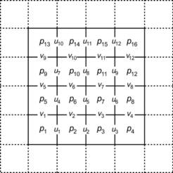
| − | In this paper the Finite Volume method (FVM) with staggered grids was applied, as described in [21], also applied by [12], with the velocities placed on the faces and the pressure on the center of the volumes. Applying this strategy avoids the numerical instabilities on the pressure solution [6,22,23]. Such grid and its ordering are represented in Figure 1 (4 to 4 volumes). | + | In this paper the Finite Volume method (FVM) with staggered grids was applied, as described in [21], also applied by [12], with the velocities placed on the faces and the pressure on the center of the volumes. Applying this strategy avoids the numerical instabilities on the pressure solution [6,22,23]. Such grid and its ordering are represented in [[#img-1|Figure 1]] (4 to 4 volumes). |
| + | <div id='img-1'></div> | ||
{| style="text-align: center; border: 1px solid #BBB; margin: 1em auto; width: auto;max-width: auto;" | {| style="text-align: center; border: 1px solid #BBB; margin: 1em auto; width: auto;max-width: auto;" | ||
|- | |- | ||
| Line 159: | Line 160: | ||
===3.2 Spatial discretization by finite volumes=== | ===3.2 Spatial discretization by finite volumes=== | ||
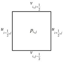
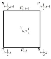
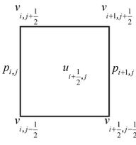
| − | Equations (1) a (3) can be integrated in each control volume described in Figure 2. | + | Equations (1) a (3) can be integrated in each control volume described in [[#img-2|Figure 2]]. |
| + | <div id='img-2'></div> | ||
{| style="text-align: center; border: 1px solid #BBB; margin: 1em auto; width: auto;max-width: auto;" | {| style="text-align: center; border: 1px solid #BBB; margin: 1em auto; width: auto;max-width: auto;" | ||
|- | |- | ||
|style="padding:10px;"|[[Image:Draft_Anunciacao_160657346-image10-c.jpeg|174px]] | |style="padding:10px;"|[[Image:Draft_Anunciacao_160657346-image10-c.jpeg|174px]] | ||
| − | | [[Image:Draft_Anunciacao_160657346-image10-c1.jpeg|center|204px]] | + | | style="padding:10px;"|[[Image:Draft_Anunciacao_160657346-image10-c1.jpeg|center|204px]] |
| − | | [[Image:Draft_Anunciacao_160657346-image10-c2.jpeg|192px]] | + | | style="padding:10px;"|[[Image:Draft_Anunciacao_160657346-image10-c2.jpeg|192px]] |
|- style="text-align: center; font-size: 75%;" | |- style="text-align: center; font-size: 75%;" | ||
| colspan="3" style="padding-bottom:10px;"| '''Figure 2'''. Control volumes | | colspan="3" style="padding-bottom:10px;"| '''Figure 2'''. Control volumes | ||
| Line 207: | Line 209: | ||
respectively. | respectively. | ||
| − | The terms of Eqs. (8), (9) and (10) were discretized applying the FVM with staggered grids, where the integrals are calculated over the control volumes defined in Figure 2, where for a matter of simplicity, the same spatial refinement was applied in all directions, that is, | + | The terms of Eqs. (8), (9) and (10) were discretized applying the FVM with staggered grids, where the integrals are calculated over the control volumes defined in Figure 2, where for a matter of simplicity, the same spatial refinement was applied in all directions, that is, <math>h_x = h_y = h</math> (uniform grids). |
In order to discretized the mass conservation, a volume centered in ''p'' was applied, Figure 2 (b), where there is: | In order to discretized the mass conservation, a volume centered in ''p'' was applied, Figure 2 (b), where there is: | ||
| Line 222: | Line 224: | ||
| − | The pressure terms were discretized applying the volumes centered in the velocity components defined in Figures 2(a) and (c), generating: | + | The pressure terms were discretized applying the volumes centered in the velocity components defined in [[#img-2|Figures 2]](a) and (c), generating: |
{| class="formulaSCP" style="width: 100%; text-align: center;" | {| class="formulaSCP" style="width: 100%; text-align: center;" | ||
| Line 333: | Line 335: | ||
===3.3 Projection methods=== | ===3.3 Projection methods=== | ||
| − | The Projection methods were introduced by [24,25], and they are characterized by the Navier-Stokes solution in two steps. Initially, an auxiliary velocity | + | The Projection methods were introduced by [24,25], and they are characterized by the Navier-Stokes solution in two steps. Initially, an auxiliary velocity <math>{\bf u}_t</math> is calculated ignoring the incompressibility condition given by Eq. (1) and the pressure term (considering <math>p = 0</math> in Eqs. (2) and (3)). In this step, a Reaction-Diffusion equation is solved by temporal discretization. In the second step, pressure is calculated by solving a Poisson equation. The most attractive property in the Projection methods is the fact that in each step a sequence of decoupled elliptical equations are solved for pressure and velocities, enabling large scale numerical simulations to be executed efficiently; however, it is not trivial to develop and analyze high order Projection methods [14]. |
| − | There are several formulations for the Projection methods, differing in the way to calculate the auxiliary velocity | + | There are several formulations for the Projection methods, differing in the way to calculate the auxiliary velocity <math>{\bf u}_t</math> and the projection step. Each of these comes from the method of [24,25], which is a Projection method with a simpler correction scheme for the pressure, which is not yet a first order method (regarding time) for pressure on norm <math>l_2</math> [14] due to the absence of the pressure gradient on the first step of the method. Goda observed that by adding the pressure gradient [26], Chorin's algorithm presents an improvement in accuracy, an idea applied by Van Kan to develop a incremental pressure-correction scheme of second order [27], which was improved by Timmemans et al. through a modification on the boundary conditions for pressure from the method mentioned previously [28]. This algorithm is known as “incremental correction for pressure on rotational form” and it will be adopted in this paper for the solution of the Navier-Stokes equations [29] . Such algorithm will be given below and it will be designated as Algorithm 1. |
| − | Furthermore, Guermond and Shen show that the incremental version on rotational form is a second order scheme for velocity on | + | Furthermore, Guermond and Shen show that the incremental version on rotational form is a second order scheme for velocity on <math>l_2</math>-, <math>l_1</math>- and <math>l_\infty</math>-norms [29]. For pressure the scheme is a second order scheme for norms <math>l_2</math>- and <math>l_1</math>-norms and 3/2 order for <math>l_\infty</math>-norms. The method consists on the following steps: |
First step: | First step: | ||
| Line 347: | Line 349: | ||
|- | |- | ||
| <math>\begin{array}{c} | | <math>\begin{array}{c} | ||
| − | \frac{3u^t-4u^n+u^{n-1}}{2\nu h_t}=\frac{\beta g}{\nu }+{\nabla }^2u^t+\frac{\nabla P^n}{\nu }\\ | + | \displaystyle\frac{3u^t-4u^n+u^{n-1}}{2\nu h_t}=\displaystyle\frac{\beta g}{\nu }+{\nabla }^2u^t+\displaystyle\frac{\nabla P^n}{\nu }\\ |
{u^t\vert }_{\partial \Omega }=b^n | {u^t\vert }_{\partial \Omega }=b^n | ||
\end{array}</math>, | \end{array}</math>, | ||
|} | |} | ||
| style="width: 5px;text-align: right;white-space: nowrap;" | (21) | | style="width: 5px;text-align: right;white-space: nowrap;" | (21) | ||
| − | |} | + | |}'''''<sup><sup>''''' |
| − | + | ||
| − | where ' | + | where 'ut is the auxiliary velocities field, un is the velocities field on the time step n, ht is the temporal refinement, Pn is pressure on the time step n and bn the boundary conditions on time step n, |
| + | <math>\beta g=u\cdot \nabla u</math> with constant <math>\beta</math> and <math>\nu =1{\mbox{/Re}}</math>. | ||
| − | Rearranging the terms on Eq. (21) , there | + | Rearranging the terms on Eq. (21) , there |
{| class="formulaSCP" style="width: 100%; text-align: center;" | {| class="formulaSCP" style="width: 100%; text-align: center;" | ||
| Line 365: | Line 367: | ||
|- | |- | ||
| <math>\begin{array}{c} | | <math>\begin{array}{c} | ||
| − | -{\nabla }^2u^t+\frac{3\mbox{Re}}{2h_t}u^t=\mbox{Re}\left(\beta g+\nabla P^n+\frac{4u^n-u^{n-1}}{2h_t}\right)\\ | + | -{\nabla }^2u^t+\displaystyle\frac{3\mbox{Re}}{2h_t}u^t=\mbox{Re}\left(\beta g+\nabla P^n+\displaystyle\frac{4u^n-u^{n-1}}{2h_t}\right)\\ |
{u^t\vert }_{\partial \Omega }=b^n | {u^t\vert }_{\partial \Omega }=b^n | ||
\end{array}</math>, | \end{array}</math>, | ||
| Line 373: | Line 375: | ||
| − | which has the form of a Reaction-Diffusion equation (Eq. (6)) for the variable | + | which has the form of a Reaction-Diffusion equation (Eq. (6)) for the variable <math>{\bf u}_t</math>, with: |
{| class="formulaSCP" style="width: 100%; text-align: center;" | {| class="formulaSCP" style="width: 100%; text-align: center;" | ||
| Line 380: | Line 382: | ||
{| style="text-align: center; margin:auto;" | {| style="text-align: center; margin:auto;" | ||
|- | |- | ||
| − | | <math>\eta =-\frac{3\mbox{Re}}{2h_t}</math> | + | | <math>\eta =-\displaystyle\frac{3\mbox{Re}}{2h_t}</math> |
|} | |} | ||
| style="width: 5px;text-align: right;white-space: nowrap;" | (23) | | style="width: 5px;text-align: right;white-space: nowrap;" | (23) | ||
| Line 393: | Line 395: | ||
{| style="text-align: center; margin:auto;" | {| style="text-align: center; margin:auto;" | ||
|- | |- | ||
| − | | <math>f=\mbox{Re}\left(\beta g+\nabla P^n+\frac{4u^n-u^{n-1}}{2h_t}\right)</math>. | + | | <math>f=\mbox{Re}\left(\beta g+\nabla P^n+\displaystyle\frac{4u^n-u^{n-1}}{2h_t}\right)</math>. |
|} | |} | ||
| style="width: 5px;text-align: right;white-space: nowrap;" | (24) | | style="width: 5px;text-align: right;white-space: nowrap;" | (24) | ||
| Line 407: | Line 409: | ||
|- | |- | ||
| <math>\begin{array}{c} | | <math>\begin{array}{c} | ||
| − | {\nabla }^2{\phi }^{n+1}=\frac{3}{2h_t}\nabla \cdot u^t\\ | + | {\nabla }^2{\phi }^{n+1}=\displaystyle\frac{3}{2h_t}\nabla \cdot u^t\\ |
| − | u^{n+1}=u^t-\frac{2h_t}{3}\nabla {\phi }^{n+1}\\ | + | u^{n+1}=u^t-\displaystyle\frac{2h_t}{3}\nabla {\phi }^{n+1}\\ |
P^{n+1}=P^n+{\phi }^{n+1}-\nu \nabla \cdot u^t | P^{n+1}=P^n+{\phi }^{n+1}-\nu \nabla \cdot u^t | ||
\end{array}</math>, | \end{array}</math>, | ||
| Line 415: | Line 417: | ||
|} | |} | ||
| − | where <math>{\phi }^{n+1}</math> is the pressure correction. | + | where <math>{\phi }^{n+1}</math>is the pressure correction. |
<div class="center" style="font-size: 75%;">'''Algorithm 1'''. Projection method | <div class="center" style="font-size: 75%;">'''Algorithm 1'''. Projection method | ||
| Line 432: | Line 434: | ||
|style="padding-left:25px;" |For ''n'' = 0, 1, 2, ..., <math>N_t</math> – 1, do: | |style="padding-left:25px;" |For ''n'' = 0, 1, 2, ..., <math>N_t</math> – 1, do: | ||
|-style="border-left: 1pt solid black;border-right: 1pt solid black;text-align: left;" | |-style="border-left: 1pt solid black;border-right: 1pt solid black;text-align: left;" | ||
| − | |style="padding-left:25px;" |'''Step 1''': given the velocities <math>u^n\mbox{, }u^{n-1}</math> and the pressure <math>P^n</math> , calculate | + | |style="padding-left:25px;" |'''Step 1''': given the velocities <math>u^n\mbox{, }u^{n-1}</math> and the pressure <math>P^n</math> , calculate <math>{\bf u}_t</math>, solving the Reaction-Diffusion equation: |
|-style="border-left: 1pt solid black;border-right: 1pt solid black;text-align: left;" | |-style="border-left: 1pt solid black;border-right: 1pt solid black;text-align: left;" | ||
|style="padding-left:25px;" |<math>-{\nabla }^2u^t+\frac{3\mbox{Re}}{2h_t}u^t=\mbox{Re}\left(\beta g+ \nabla P^n+\frac{4u^n-u^{n-1}}{2h_t}\right)</math> | |style="padding-left:25px;" |<math>-{\nabla }^2u^t+\frac{3\mbox{Re}}{2h_t}u^t=\mbox{Re}\left(\beta g+ \nabla P^n+\frac{4u^n-u^{n-1}}{2h_t}\right)</math> | ||
|-style="border-left: 1pt solid black;border-right: 1pt solid black;text-align: left;" | |-style="border-left: 1pt solid black;border-right: 1pt solid black;text-align: left;" | ||
| − | |style="padding-left:25px;" |'''Step 2''': Given the velocity | + | |style="padding-left:25px;" |'''Step 2''': Given the velocity <math>{\bf u}_t</math>, calculate <math>{\phi }^{n+1}</math> , solving the Poisson equation: |
|-style="border-left: 1pt solid black;border-right: 1pt solid black;text-align: left;" | |-style="border-left: 1pt solid black;border-right: 1pt solid black;text-align: left;" | ||
|style="padding-left:25px;" |<math>{\nabla }^2{\phi }^{n+1}=\frac{3}{2h_t}\nabla \cdot u^t</math> | |style="padding-left:25px;" |<math>{\nabla }^2{\phi }^{n+1}=\frac{3}{2h_t}\nabla \cdot u^t</math> | ||
| Line 451: | Line 453: | ||
| − | If the time step | + | If the time step <math>h_t</math> is too large in relation to spatial refinement (<math>h_x</math> and <math>h_y</math>), the simulations can become unstable [30]. The criterion applied in this paper to avoid instabilities is given by [12,30]: |
{| class="formulaSCP" style="width: 100%; text-align: center;" | {| class="formulaSCP" style="width: 100%; text-align: center;" | ||
| Line 458: | Line 460: | ||
{| style="text-align: center; margin:auto;" | {| style="text-align: center; margin:auto;" | ||
|- | |- | ||
| − | | <math>h_t<\frac{1}{2\mbox{Re}}\frac{h_x^2h_y^2}{h_x^2+h_y^2}</math>. | + | | <math>h_t<\displaystyle\frac{1}{2\mbox{Re}}\displaystyle\frac{h_x^2h_y^2}{h_x^2+h_y^2}</math>. |
|} | |} | ||
| style="width: 5px;text-align: right;white-space: nowrap;" | (26) | | style="width: 5px;text-align: right;white-space: nowrap;" | (26) | ||
| Line 464: | Line 466: | ||
| − | Since this paper considers | + | Since this paper considers <math>h_x = h_y = h</math>, the criterion can be rewritten as |
{| class="formulaSCP" style="width: 100%; text-align: center;" | {| class="formulaSCP" style="width: 100%; text-align: center;" | ||
| Line 471: | Line 473: | ||
{| style="text-align: center; margin:auto;" | {| style="text-align: center; margin:auto;" | ||
|- | |- | ||
| − | | <math>h_t<\frac{h^2}{4\mbox{Re}}</math>. | + | | <math>h_t<\displaystyle\frac{h^2}{4\mbox{Re}}</math>. |
|} | |} | ||
| style="width: 5px;text-align: right;white-space: nowrap;" | (27) | | style="width: 5px;text-align: right;white-space: nowrap;" | (27) | ||
| Line 484: | Line 486: | ||
{| style="text-align: center; margin:auto;" | {| style="text-align: center; margin:auto;" | ||
|- | |- | ||
| − | | <math>{\int }_{\Omega }{\nabla }^2{\phi }^{n+1}={\int }_{\Omega }\frac{1}{h_t}\nabla \cdot u^{n+1}=</math><math>0</math>. | + | | <math>{\int }_{\Omega }{\nabla }^2{\phi }^{n+1}={\int }_{\Omega }\displaystyle\frac{1}{h_t}\nabla \cdot u^{n+1}=</math><math>0</math>. |
|} | |} | ||
| style="width: 5px;text-align: right;white-space: nowrap;" | (28) | | style="width: 5px;text-align: right;white-space: nowrap;" | (28) | ||
| Line 506: | Line 508: | ||
|} | |} | ||
| − | where ''b'' and <math>f\in R^n</math> where ''b'' can be ''u'', ''v'' or <math>\phi </math> , according to steps 1 and 2 on | + | where ''b'' and <math>f\in R^n</math> where ''b'' can be ''u'', ''v'' or <math>\phi </math> , according to steps 1 and 2 on Algorithm 1. |
===4.1 Gauss-Seidel method (GS)=== | ===4.1 Gauss-Seidel method (GS)=== | ||
| Line 552: | Line 554: | ||
where <math>B=P^{-1}N</math>, <math>N=P-A</math>, and ''B'' is called the iteration matrix of the method given by Eq. (32). | where <math>B=P^{-1}N</math>, <math>N=P-A</math>, and ''B'' is called the iteration matrix of the method given by Eq. (32). | ||
| − | If the diagonal entries of ''A'' are non-zeros, the unknown corresponding value can be isolated in each equation, resulting in the Gauss-Seidel method, given an initial estimate | + | If the diagonal entries of ''A'' are non-zeros, the unknown corresponding value can be isolated in each equation, resulting in the Gauss-Seidel method, given an initial estimate <math>b^{(0)}</math>: |
{| class="formulaSCP" style="width: 100%; text-align: center;" | {| class="formulaSCP" style="width: 100%; text-align: center;" | ||
| Line 566: | Line 568: | ||
===4.2 Preconditioned Conjugated Gradient (PCG)=== | ===4.2 Preconditioned Conjugated Gradient (PCG)=== | ||
| − | Descent methods are based on obtaining a solution ''b'' for a system of the type given by Eq. (29) by the minimization property of an appropriate norm for the error. From an initial estimate | + | Descent methods are based on obtaining a solution ''b'' for a system of the type given by Eq. (29) by the minimization property of an appropriate norm for the error. From an initial estimate <math>b^{(0)}</math>, these methods determine a solution for the problem by diminishing the error. |
| − | The vectorial norm being given by <math>{\Vert b\Vert }_2=\langle b,Sb\rangle </math>, where <math>S\in R^{nxn}</math> is a positive defined symmetrical matrix. Considering the residual equation | + | The vectorial norm being given by <math>{\Vert b\Vert }_2=\langle b,Sb\rangle </math>, where <math>S\in R^{nxn}</math> is a positive defined symmetrical matrix. Considering the residual equation <math>Ae^{(k)} = r^{(k)}</math>, it can be deduced that: |
{| class="formulaSCP" style="width: 100%; text-align: center;" | {| class="formulaSCP" style="width: 100%; text-align: center;" | ||
| Line 575: | Line 577: | ||
{| style="text-align: center; margin:auto;" | {| style="text-align: center; margin:auto;" | ||
|- | |- | ||
| − | | <math>{\Vert e^{\left(k\right)}\Vert }_2=\langle e^{\left(k\right)},Se^{\left(k\right)}\rangle =</math><math>\langle r^{\left(k\right)},Rr^{\left(k\right)}\rangle </math> , | + | | <math>{\Vert e^{\left(k\right)}\Vert }_2=\langle e^{\left(k\right)},Se^{\left(k\right)}\rangle =</math><math>\langle r^{\left(k\right)},Rr^{\left(k\right)}\rangle </math>, |
|} | |} | ||
| style="width: 5px;text-align: right;white-space: nowrap;" | (34) | | style="width: 5px;text-align: right;white-space: nowrap;" | (34) | ||
| Line 582: | Line 584: | ||
where <math>R=A^{-T}SA^{-1}</math>, which means that minimizing the error equals minimizing the residue in the same norm [7]. | where <math>R=A^{-T}SA^{-1}</math>, which means that minimizing the error equals minimizing the residue in the same norm [7]. | ||
| − | On the Descent method one starts from an initial estimate | + | On the Descent method one starts from an initial estimate <math>b^{(0)}</math> for the solution and a succession of vectors <math>b^{1} ,\cdots , b^{(k)} ,\cdots </math> is generated, moving successively towards diminishing the error, making this succession converge to ''b''. |
| − | One of the ways to choose the best direction in each point | + | One of the ways to choose the best direction in each point <math>b^{(k)}</math> would be to choose the direction of <math>p^{(k)}</math> which is lined up with the direction of the function gradient, but in the opposite orientation (Gradients method). |
Thus, the iterative expression of the Gradients methods is given by [7]: | Thus, the iterative expression of the Gradients methods is given by [7]: | ||
| Line 600: | Line 602: | ||
where <math>G_k=I-{\alpha }_kS</math> and <math>c_k={\alpha }_kSA^{-1}f</math>, <math>{\alpha }_k</math> being a constant. | where <math>G_k=I-{\alpha }_kS</math> and <math>c_k={\alpha }_kSA^{-1}f</math>, <math>{\alpha }_k</math> being a constant. | ||
| − | Conjugate Gradient method (CG) is an iterative descent method applied in cases where the iteration matrix ''A ''is a symmetric positive definite matrix. This method demands a more careful choice of the descent directions | + | Conjugate Gradient method (CG) is an iterative descent method applied in cases where the iteration matrix ''A ''is a symmetric positive definite matrix. This method demands a more careful choice of the descent directions <math>p^{(k)}</math>. |
| − | In order to exemplify it, consider a two-dimensional problem. The lines <math>{\Vert e^{\left(k\right)}\Vert }_2={\Vert r^{\left(k\right)}\Vert }_2=</math><math>\mbox{constante}</math>, are concentric ellipses with the center in ''b'', as illustrated in Figure 3. | + | In order to exemplify it, consider a two-dimensional problem. The lines <math>{\Vert e^{\left(k\right)}\Vert }_2={\Vert r^{\left(k\right)}\Vert }_2=</math><math>\mbox{constante}</math>, are concentric ellipses with the center in ''b'', as illustrated in [[#img-3|Figure 3]]. |
| + | <div id='img-3'></div> | ||
{| style="text-align: center; border: 1px solid #BBB; margin: 1em auto; width: auto;max-width: auto;" | {| style="text-align: center; border: 1px solid #BBB; margin: 1em auto; width: auto;max-width: auto;" | ||
|- | |- | ||
| Line 612: | Line 615: | ||
| − | Supposing there is an initial estimate | + | Supposing there is an initial estimate <math>b^{(0)}</math>, according to the Gradient method, one can start from this point and research the minimum of <math>{\Vert e^{\left(k\right)}\Vert }_2</math>, across the direction <math>r^{(0)}</math>, obtaining <math>b^{(1)}</math>. Observing Figure 3, it can be verified that the best progression of <math>b^{(1)}</math> would not be the more inclined direction, but the direction <math>p^{(1)}</math> which points to the center of the ellipse. |
| − | In fact, the new minimizing point | + | In fact, the new minimizing point <math>b^{(2)}</math> would coincide with the exact solution of ''b'', and thus the iterative process would end with just two iterations. Therefore a direction <math>p^{(1)}</math> can be chosen as: |
{| class="formulaSCP" style="width: 100%; text-align: center;" | {| class="formulaSCP" style="width: 100%; text-align: center;" | ||
| Line 688: | Line 691: | ||
where <math>cond_2A={\Vert A\Vert }_2\cdot {\Vert A^{-1}\Vert }_2</math>. | where <math>cond_2A={\Vert A\Vert }_2\cdot {\Vert A^{-1}\Vert }_2</math>. | ||
| − | Thus, it can be noticed that the CG method, theoretically, calculates the exact solution in ''n'' iterations, which is not verified in practice due to the application of this method in finite precision arithmetic’s and the introduction of rounding errors which destroy the exact conjugacy of the direction | + | Thus, it can be noticed that the CG method, theoretically, calculates the exact solution in ''n'' iterations, which is not verified in practice due to the application of this method in finite precision arithmetic’s and the introduction of rounding errors which destroy the exact conjugacy of the direction <math>p^{(k)}</math> and the exact orthogonality of the residues <math>r^{(k)}</math>. Thus, this method takes a typical iterative form. |
One way to make this iterative method faster consists in transforming the system <math>Ab=f</math> into an equivalent system, where the matrix has a more favorable conditioning number. According to Eq. (41), if it is possible to reduce <math>cond_2A</math>, consequently a fast convergence is achieved. | One way to make this iterative method faster consists in transforming the system <math>Ab=f</math> into an equivalent system, where the matrix has a more favorable conditioning number. According to Eq. (41), if it is possible to reduce <math>cond_2A</math>, consequently a fast convergence is achieved. | ||
| Line 706: | Line 709: | ||
The system now corresponds, therefore, to <math>\overline{A}\overline{b}=\overline{f}</math>, with <math>\overline{A}=PAQ</math>, <math>\overline{b}=Q^{-1}b</math> and <math>\overline{f}=Pf</math>, the matrixes ''P'' and ''Q'' having to be chosen in the way that provides the best convergence properties to the matrix in relation to the original matrix ''A''. This procedure is known as preconditioning of the original equations system, ''P'' and ''Q'' being known by the name of preconditioning matrixes. | The system now corresponds, therefore, to <math>\overline{A}\overline{b}=\overline{f}</math>, with <math>\overline{A}=PAQ</math>, <math>\overline{b}=Q^{-1}b</math> and <math>\overline{f}=Pf</math>, the matrixes ''P'' and ''Q'' having to be chosen in the way that provides the best convergence properties to the matrix in relation to the original matrix ''A''. This procedure is known as preconditioning of the original equations system, ''P'' and ''Q'' being known by the name of preconditioning matrixes. | ||
| − | Considering that in the CG method the transformed matrix has to keep being a symmetric positive definite matrix, the preconditioning will also have to preserve this property. In fact, it can be obtained making | + | Considering that in the CG method the transformed matrix has to keep being a symmetric positive definite matrix, the preconditioning will also have to preserve this property. In fact, it can be obtained making <math>P = S</math> and <math>Q = P^ T = S^T</math>, and in this manner, it can be concluded that <math>\overline{A}\overline{b}=\overline{f}</math>, <math>\overline{A}=SAS^T</math>, <math>\overline{b}=S^{-T}b</math> and <math>\overline{f}=Sf</math>. |
Thus, it can be verified that <math>{\overline{p}}^{\left(0\right)}={\overline{r}}^{\left(0\right)}=</math><math>\overline{f}-\overline{A}{\overline{b}}^{\left(0\right)}=</math><math>Sr^{\left(0\right)}.</math> On the other hand, choosing <math>p^{\left(0\right)}=S^T{\overline{p}}^{\left(0\right)}=</math><math>S^T{\overline{r}}^{\left(0\right)}=S^TSr^{\left(0\right)},</math> there is <math>\langle {\overline{p}}^{\left(0\right)},\overline{A}{\overline{p}}^{\left(0\right)}\rangle =</math><math>\langle p^{\left(0\right)},Ap^{\left(0\right)}\rangle ,</math> the relation <math>\langle {\overline{r}}^{\left(0\right)},{\overline{r}}^{\left(0\right)}\rangle =</math><math>\langle {\overline{r}}^{\left(0\right)},r^{\left(0\right)}\rangle </math> also being valid, with | Thus, it can be verified that <math>{\overline{p}}^{\left(0\right)}={\overline{r}}^{\left(0\right)}=</math><math>\overline{f}-\overline{A}{\overline{b}}^{\left(0\right)}=</math><math>Sr^{\left(0\right)}.</math> On the other hand, choosing <math>p^{\left(0\right)}=S^T{\overline{p}}^{\left(0\right)}=</math><math>S^T{\overline{r}}^{\left(0\right)}=S^TSr^{\left(0\right)},</math> there is <math>\langle {\overline{p}}^{\left(0\right)},\overline{A}{\overline{p}}^{\left(0\right)}\rangle =</math><math>\langle p^{\left(0\right)},Ap^{\left(0\right)}\rangle ,</math> the relation <math>\langle {\overline{r}}^{\left(0\right)},{\overline{r}}^{\left(0\right)}\rangle =</math><math>\langle {\overline{r}}^{\left(0\right)},r^{\left(0\right)}\rangle </math> also being valid, with | ||
| Line 891: | Line 894: | ||
In this paper, moreover, the V-Cycle was applied, for its computational efficiency. The equations of Poisson and Reaction-Diffusion being linear, the correction scheme (CS) was applied, which transfers only the residues to the coarser grids [5,6]. The coarsening ratio, considering uniform grids, is defined as ''r'' = ''H''/''h'', where ''h ''represents the size of the spacing of the fine grid, <math>{\Omega }^h</math> , (also called the dimension of the fine grid elements), and ''H'' the size at the element of the next coarser grid, <math>{\Omega }^H</math> . | In this paper, moreover, the V-Cycle was applied, for its computational efficiency. The equations of Poisson and Reaction-Diffusion being linear, the correction scheme (CS) was applied, which transfers only the residues to the coarser grids [5,6]. The coarsening ratio, considering uniform grids, is defined as ''r'' = ''H''/''h'', where ''h ''represents the size of the spacing of the fine grid, <math>{\Omega }^h</math> , (also called the dimension of the fine grid elements), and ''H'' the size at the element of the next coarser grid, <math>{\Omega }^H</math> . | ||
| − | Figure 4 illustrates the cycle-V with CS for five grids. The superscripts ''h'', 2''h'' , 4''h'', ... indicate the grid where the vectors and matrixes are defined, the smoothing numbers (S) being achieved in the restriction process (R) (pre-smoothing) and prolongation (P) (post-smoothing) being represented, respectively, by <math>{\nu }_1</math> and <math>{\nu }_2</math>. | + | [[#img-4|Figure 4]] illustrates the cycle-V with CS for five grids. The superscripts ''h'', 2''h'' , 4''h'', ... indicate the grid where the vectors and matrixes are defined, the smoothing numbers (S) being achieved in the restriction process (R) (pre-smoothing) and prolongation (P) (post-smoothing) being represented, respectively, by <math>{\nu }_1</math> and <math>{\nu }_2</math>. |
| + | <div id='img-4'></div> | ||
{| style="text-align: center; border: 1px solid #BBB; margin: 1em auto; width: auto;max-width: auto;" | {| style="text-align: center; border: 1px solid #BBB; margin: 1em auto; width: auto;max-width: auto;" | ||
|- | |- | ||
| Line 917: | Line 921: | ||
:4) Preconditioned Conjugated Gradient with Multigrid and ILU solver (PCG-MG-ILU). | :4) Preconditioned Conjugated Gradient with Multigrid and ILU solver (PCG-MG-ILU). | ||
| − | In all simulations and for all the variables of interest, the stop criterion applied was the nondimensionalized residue | + | In all simulations and for all the variables of interest, the stop criterion applied was the nondimensionalized residue <math>l_2</math>-norm based on the initial estimate, given by: |
{| class="formulaSCP" style="width: 100%; text-align: center;" | {| class="formulaSCP" style="width: 100%; text-align: center;" | ||
| Line 929: | Line 933: | ||
|} | |} | ||
| − | where | + | where <math>r^{\left(k\right)}</math> is the residue on the current iteration, <math>r^{\left(0\right)}</math> is the residue of the initial estimate, and ε is the tolerance. |
| − | In this paper the null vector was utilized as the initial estimate for all the variables of interest and with the use of double precision. The standard coarsening ratio was utilized, that is , | + | In this paper the null vector was utilized as the initial estimate for all the variables of interest and with the use of double precision. The standard coarsening ratio was utilized, that is , <math>r = 2</math> [5], where the Multigrid method started from the finest grid and got to the coarsest grid possible, that is, the grid with <math>N= 2\times 2</math> volumes. The number of unknowns in the finest grids was: <math>N = 16\times</math>16, 32<math>\times</math>32, 64<math>\times</math>64, 128<math>\times</math>128, 256<math>\times</math>256, 512<math>\times</math>512 and 1024<math>\times</math>1024. The number of pre- and post-smoothing was equals to <math>\nu ={\nu }_1={\nu }_2=3</math>. |
The computer utilized for the simulations has an Intel Core i7-5500 processor, a 2.40 Ghz CPU, 16.0 Gb memory and a 64 bits Windows 10 operational system. | The computer utilized for the simulations has an Intel Core i7-5500 processor, a 2.40 Ghz CPU, 16.0 Gb memory and a 64 bits Windows 10 operational system. | ||
| Line 937: | Line 941: | ||
Four parameters were analyzed in order to compare the four methodologies: | Four parameters were analyzed in order to compare the four methodologies: | ||
| − | :* | + | :* <math>l_\infty</math>-norm for numerical error (<math>||E||_\infty</math>); |
| − | :* | + | :* <math>l_2</math>-norm for nondimensionalized residue based on the initial estimate (Eq. (54)); |
:* Empirical convergence factor, defined as [6]: | :* Empirical convergence factor, defined as [6]: | ||
| Line 948: | Line 952: | ||
{| style="text-align: center; margin:auto;" | {| style="text-align: center; margin:auto;" | ||
|- | |- | ||
| − | | <math>q^{\mbox{(}k\mbox{)}}=\frac{{\Vert r^{\left(k\right)}\Vert }_2}{{\Vert r^{\left(k-1\right)}\Vert }_2}</math> | + | | <math>q^{\mbox{(}k\mbox{)}}=\displaystyle\frac{{\Vert r^{\left(k\right)}\Vert }_2}{{\Vert r^{\left(k-1\right)}\Vert }_2}</math> |
|} | |} | ||
| style="width: 5px;text-align: right;white-space: nowrap;" | (55) | | style="width: 5px;text-align: right;white-space: nowrap;" | (55) | ||
| Line 961: | Line 965: | ||
This phase it is intended to determine the best method to solve the Poisson equation, which models pressure, determining a method to solve the velocities equations. In this case, MG-GS, MG-ILU, PCG-MG-GS and PCG-MG-ILU were utilized for pressure and MG-GS for the velocities. | This phase it is intended to determine the best method to solve the Poisson equation, which models pressure, determining a method to solve the velocities equations. In this case, MG-GS, MG-ILU, PCG-MG-GS and PCG-MG-ILU were utilized for pressure and MG-GS for the velocities. | ||
| − | The behavior of the | + | The behavior of the <math>l_\infty</math>-norm was initially evaluated for the four studied methods, where it could be noticed that all of them presented a reduction in the numerical error norm with the increase in the size of the problem; a desirable characteristic in a convergent numerical method ([[#img-5|Figure 5]]). |
| + | <div id='img-5'></div> | ||
{| style="text-align: center; border: 1px solid #BBB; margin: 1em auto; width: auto;max-width: auto;" | {| style="text-align: center; border: 1px solid #BBB; margin: 1em auto; width: auto;max-width: auto;" | ||
|- | |- | ||
| Line 971: | Line 976: | ||
| − | Figure 6 presents the number of iterations necessary in order to reach the stop criterion for the problem with <math>N' = 1024\times 1024</math>. Based on this figure, it can be noticed that PCG-MG-ILU reached the stop criterion in a lower number of iterations. | + | [[#img-6|Figure 6]] presents the number of iterations necessary in order to reach the stop criterion for the problem with <math>N' = 1024\times 1024</math>. Based on this figure, it can be noticed that PCG-MG-ILU reached the stop criterion in a lower number of iterations. |
| + | <div id='img-6'></div> | ||
{| style="text-align: center; border: 1px solid #BBB; margin: 1em auto; width: auto;max-width: auto;" | {| style="text-align: center; border: 1px solid #BBB; margin: 1em auto; width: auto;max-width: auto;" | ||
|- | |- | ||
|style="padding:10px;"|[[Image:Draft_Anunciacao_160657346-image127.jpeg|456px]] | |style="padding:10px;"|[[Image:Draft_Anunciacao_160657346-image127.jpeg|456px]] | ||
|- style="text-align: center; font-size: 75%;" | |- style="text-align: center; font-size: 75%;" | ||
| − | | colspan="1" style="padding | + | | colspan="1" style="padding:10px;"| '''Figure 6'''. <math>l_2</math>-norm for the nondimensionalized residue by the norm of initial estimate ''versus'' number of |
| − | + | ||
| − | estimate ''versus'' number of | + | |
iterations for the problem with <math>N' = 1024\times 1024</math> for ''p'' | iterations for the problem with <math>N' = 1024\times 1024</math> for ''p'' | ||
|} | |} | ||
| − | Figure 7 illustrates the behavior of the empirical convergence factor with the increase of the size of the problem. Based on this figure, it can be claimed again that the PCG-MG-ILU methodology presented the best results, since it is the one that generated the best values for the convergence factors, that is, values near to zero [5,34]. | + | [[#img-7|Figure 7]] illustrates the behavior of the empirical convergence factor with the increase of the size of the problem. Based on this figure, it can be claimed again that the PCG-MG-ILU methodology presented the best results, since it is the one that generated the best values for the convergence factors, that is, values near to zero [5,34]. |
| + | <div id='img-7'></div> | ||
{| style="text-align: center; border: 1px solid #BBB; margin: 1em auto; width: auto;max-width: auto;" | {| style="text-align: center; border: 1px solid #BBB; margin: 1em auto; width: auto;max-width: auto;" | ||
|- | |- | ||
| Line 994: | Line 999: | ||
| − | Figure 8 illustrates the behavior of the CPU time (in seconds) of the simulations with the increase of the size of the problem. It can be noticed that the computational times became very close, with a slight advantage for the PCG-MG-ILU methodology, which can be confirmed in sequence. | + | [[#img-8|Figure 8]] illustrates the behavior of the CPU time (in seconds) of the simulations with the increase of the size of the problem. It can be noticed that the computational times became very close, with a slight advantage for the PCG-MG-ILU methodology, which can be confirmed in sequence. |
| + | <div id='img-8'></div> | ||
{| style="text-align: center; border: 1px solid #BBB; margin: 1em auto; width: auto;max-width: auto;" | {| style="text-align: center; border: 1px solid #BBB; margin: 1em auto; width: auto;max-width: auto;" | ||
|- | |- | ||
| Line 1,017: | Line 1,023: | ||
| − | Table 1 shows the Speed-up of the three methods MG-GS, MG-ILU and PCG-MG-GS in relation to the PCG-MG-ILU method. | + | [[#tab-1|Table 1]] shows the Speed-up of the three methods MG-GS, MG-ILU and PCG-MG-GS in relation to the PCG-MG-ILU method. |
<div class="center" style="font-size: 75%;">'''Table 1'''. Speed-up values for MG-GS, MG-ILU and PCG-MG-GS in relation to PCG-MG-ILU | <div class="center" style="font-size: 75%;">'''Table 1'''. Speed-up values for MG-GS, MG-ILU and PCG-MG-GS in relation to PCG-MG-ILU | ||
</div> | </div> | ||
| − | {| style="margin: 1em auto 0.1em auto;border-collapse: collapse;font-size:85%;width: | + | <div id='tab-1'></div> |
| + | {| class="wikitable" style="margin: 1em auto 0.1em auto;border-collapse: collapse;font-size:85%;width:auto;" | ||
| + | |-style="text-align:center" | ||
| + | ! ''N'' !! '''MG-GS''' !! '''MG-ILU''' !! '''PCG-MG-GS''' | ||
|- | |- | ||
| − | | style=" | + | | style="text-align: center;vertical-align: top;"|16<math>\times</math>16 |
| − | + | | style="text-align: center;vertical-align: top;"|1 | |
| − | + | | style="text-align: center;vertical-align: top;"|1 | |
| − | + | | style="text-align: center;vertical-align: top;"|1 | |
| − | + | ||
| − | + | ||
| − | | style=" | + | |
| − | | style=" | + | |
| − | | style=" | + | |
|- | |- | ||
| style="text-align: center;vertical-align: top;"|32<math>\times</math>32 | | style="text-align: center;vertical-align: top;"|32<math>\times</math>32 | ||
| Line 1,059: | Line 1,063: | ||
| style="text-align: center;vertical-align: top;"|1.160 | | style="text-align: center;vertical-align: top;"|1.160 | ||
|- | |- | ||
| − | | style=" | + | | style="text-align: center;vertical-align: top;"|1024<math>\times</math>1024 |
| − | | style=" | + | | style="text-align: center;vertical-align: top;"|1.074 |
| − | | style=" | + | | style="text-align: center;vertical-align: top;"|1.194 |
| − | | style=" | + | | style="text-align: center;vertical-align: top;"|1.167 |
|} | |} | ||
| Line 1,074: | Line 1,078: | ||
In this phase, it is intended to determine the best method to solve the Reaction-Diffusion equations, which model the velocities ''u'' and ''v'', determining the best method for pressure presented in the previous section, which was PCG-MG-ILU. Since the results for the velocities ''u'' and ''v'' for all the parameters are similar, it was chose to display only the results for ''u''. | In this phase, it is intended to determine the best method to solve the Reaction-Diffusion equations, which model the velocities ''u'' and ''v'', determining the best method for pressure presented in the previous section, which was PCG-MG-ILU. Since the results for the velocities ''u'' and ''v'' for all the parameters are similar, it was chose to display only the results for ''u''. | ||
| − | Figure 9 shows the behavior of the numerical error ''versus'' the size of the problem, for the several solution methods. It can be noticed that the four studied methods presented an expected characteristic for the convergent iterative methods, that is, the decrease in the numerical error with the increase in the size of the problem. It can also be noticed that the presented error have values which are very close among themselves. | + | [[#img-9|Figure 9]] shows the behavior of the numerical error ''versus'' the size of the problem, for the several solution methods. It can be noticed that the four studied methods presented an expected characteristic for the convergent iterative methods, that is, the decrease in the numerical error with the increase in the size of the problem. It can also be noticed that the presented error have values which are very close among themselves. |
| + | <div id='img-9'></div> | ||
{| style="text-align: center; border: 1px solid #BBB; margin: 1em auto; width: auto;max-width: auto;" | {| style="text-align: center; border: 1px solid #BBB; margin: 1em auto; width: auto;max-width: auto;" | ||
|- | |- | ||
|style="padding:10px;"| [[Image:Draft_Anunciacao_160657346-image131.jpeg|432px]] | |style="padding:10px;"| [[Image:Draft_Anunciacao_160657346-image131.jpeg|432px]] | ||
|- style="text-align: center; font-size: 75%;" | |- style="text-align: center; font-size: 75%;" | ||
| − | | colspan="1" style="padding | + | | colspan="1" style="padding:10px;"| '''Figure 9'''. <math>l_\infty </math>-norm for the numerical error (<math>||E||_\infty</math>) ''versus'' size of the problem (''N'') for ''p'' |
|} | |} | ||
| − | Figure 10 displays the behavior of <math>_2</math>-norm of the nondimensionalized residue by <math>l_2</math>-norm of the initial estimate in function of the number of iterations for the problem with <math>N = 1024\times 1024</math> volumes. Based on this figure, it can be noticed that the PCG-MG-ILU and the MG-ILU methods were the ones which achieved the stop criterion in the lowest number of iterations. | + | [[#img-10|Figure 10]] displays the behavior of <math>_2</math>-norm of the nondimensionalized residue by <math>l_2</math>-norm of the initial estimate in function of the number of iterations for the problem with <math>N = 1024\times 1024</math> volumes. Based on this figure, it can be noticed that the PCG-MG-ILU and the MG-ILU methods were the ones which achieved the stop criterion in the lowest number of iterations. |
| − | {| style="text-align: center; border: 1px solid #BBB; margin: 1em auto; width: auto;max-width: | + | <div id='img-10'></div> |
| + | {| style="text-align: center; border: 1px solid #BBB; margin: 1em auto; width: auto;max-width: 50%;" | ||
|- | |- | ||
|style="padding:10px;"| [[Image:Draft_Anunciacao_160657346-image132.jpeg|456px]] | |style="padding:10px;"| [[Image:Draft_Anunciacao_160657346-image132.jpeg|456px]] | ||
|- style="text-align: center; font-size: 75%;" | |- style="text-align: center; font-size: 75%;" | ||
| − | | colspan="1" style="padding | + | | colspan="1" style="padding:10px;"| '''Figure 10'''. <math>l_2</math>-norm for the nondimensionalized residue by <math>l_2</math>-norm of the initial estimate ''versus'' number of iterations for the problem with <math>N = 1024\times 1024</math> for ''u'' |
|} | |} | ||
| − | Figure 11 illustrates the behavior of the empirical convergence factor in function of the size of the problem. Based on this figure, it can be concluded that the PCG-MG-ILU method presented the best results, since it generated the best values for the convergence factors (closest values to zero), besides decreasing its value with the increase of the size of the problem. | + | [[#img-11|Figure 11]] illustrates the behavior of the empirical convergence factor in function of the size of the problem. Based on this figure, it can be concluded that the PCG-MG-ILU method presented the best results, since it generated the best values for the convergence factors (closest values to zero), besides decreasing its value with the increase of the size of the problem. |
| + | <div id='img-11'></div> | ||
{| style="text-align: center; border: 1px solid #BBB; margin: 1em auto; width: auto;max-width: auto;" | {| style="text-align: center; border: 1px solid #BBB; margin: 1em auto; width: auto;max-width: auto;" | ||
|- | |- | ||
| Line 1,104: | Line 1,111: | ||
| − | Figure 12 shows the CPU times (in seconds) of the simulations with the increase of the size of the problem. Based on this figure, it can be noticed that the computational times were very close, with a slight advantage for the PCG-MG-ILU methodology, which can be confirmed in the results presented in the sequence. | + | [[#img-12|Figure 12]] shows the CPU times (in seconds) of the simulations with the increase of the size of the problem. Based on this figure, it can be noticed that the computational times were very close, with a slight advantage for the PCG-MG-ILU methodology, which can be confirmed in the results presented in the sequence. |
| + | <div id='img-12'></div> | ||
{| style="text-align: center; border: 1px solid #BBB; margin: 1em auto; width: auto;max-width: auto;" | {| style="text-align: center; border: 1px solid #BBB; margin: 1em auto; width: auto;max-width: auto;" | ||
|- | |- | ||
| Line 1,114: | Line 1,122: | ||
| − | Table 2 presents the Speed-up (Eq.(56)) of the MG-GS, MG-ILU and PCG-MG-GS methods in relation to the PCG-MG-ILU method. In this table, it can be confirmed that the CPU times are close among themselves, but there is an advantage with the use of PCG-MG-ILU, that is, the method that most accelerated the convergence of the iterative process for the presented problem. | + | [[#tab-2|Table 2]] presents the Speed-up (Eq.(56)) of the MG-GS, MG-ILU and PCG-MG-GS methods in relation to the PCG-MG-ILU method. In this table, it can be confirmed that the CPU times are close among themselves, but there is an advantage with the use of PCG-MG-ILU, that is, the method that most accelerated the convergence of the iterative process for the presented problem. |
<div class="center" style="font-size: 75%;">'''Table 2'''. Values of Speed-up for MG-GS, MG-ILU and PCG-MG-GS in relation to PCG-MG-ILU | <div class="center" style="font-size: 75%;">'''Table 2'''. Values of Speed-up for MG-GS, MG-ILU and PCG-MG-GS in relation to PCG-MG-ILU | ||
</div> | </div> | ||
| − | {| style=" | + | <div id='tab-2'></div> |
| + | {| class="wikitable" style="margin: 1em auto 0.1em auto;border-collapse: collapse;font-size:85%;width:auto;" | ||
| + | |-style="text-align:center" | ||
| + | ! style="text-align: center;"|''N'' !! style="text-align: center;vertical-align: top;"|'''MG-GS''' !! style="text-align: center;vertical-align: top;"|'''MG-ILU''' !! style="text-align: center;vertical-align: top;"|'''PCG-MG-GS''' | ||
|- | |- | ||
| − | | style=" | + | | style="text-align: center;vertical-align: top;"|16<math>\times</math>16 |
| − | + | | style="text-align: center;vertical-align: top;"|1 | |
| − | + | | style="text-align: center;vertical-align: top;"|1 | |
| − | + | | style="text-align: center;vertical-align: top;"|1 | |
| − | + | ||
| − | + | ||
| − | | style=" | + | |
| − | | style=" | + | |
| − | | style=" | + | |
|- | |- | ||
| style="text-align: center;vertical-align: top;"|32<math>\times</math>32 | | style="text-align: center;vertical-align: top;"|32<math>\times</math>32 | ||
| Line 1,156: | Line 1,162: | ||
| style="text-align: center;vertical-align: top;"|1.524 | | style="text-align: center;vertical-align: top;"|1.524 | ||
|- | |- | ||
| − | | style=" | + | | style="text-align: center;vertical-align: top;"|1024<math>\times</math>1024 |
| − | | style=" | + | | style="text-align: center;vertical-align: top;"|1.337 |
| − | | style=" | + | | style="text-align: center;vertical-align: top;"|1.228 |
| − | | style=" | + | | style="text-align: center;vertical-align: top;"|1.535 |
|} | |} | ||
| − | ==5.4 Algorithm== | + | ===5.4 Algorithm=== |
| − | After the tests of the two previous phases (sections 5.2 and 5.3), whose objective was to identify the best methods for the solution of the equations for the variables | + | After the tests of the two previous phases (sections 5.2 and 5.3), whose objective was to identify the best methods for the solution of the equations for the variables <math>p</math> (Poisson equation) and <math>u</math> and <math>v</math> (Reaction-Diffusion equations), we get to the point where the best methods were applied simultaneously to solve the Navier-Stokes equations. |
| − | The results presented below are compared the classic Gauss-Seidel (GS) method in its singlegrid version (only grid method) so that the gains can be measured when using the proposed algorithm (adaptation of the Projection method presented in Algorithm 1), that is, using the PCG-MG-ILU solver in the solution of the linear systems given in steps 1 and 2 of Algorithm 1 | + | The results presented below are compared the classic Gauss-Seidel (GS) method in its singlegrid version (only grid method) so that the gains can be measured when using the proposed algorithm (adaptation of the Projection method presented in Algorithm 1), that is, using the PCG-MG-ILU solver in the solution of the linear systems given in steps 1 and 2 of Algorithm 1. |
| − | Figure 13 presents the behavior of | + | [[#img-13|Figure 13]] presents the behavior of <math>l_2</math>-norm of the nondimensionalized residue by the initial estimate in function of the number of iterations for the problem with <math>N = 128\times128</math> volumes for the variables <math>u</math>, <math>v</math> and <math>p</math>. Based on this figure, it can be noticed that the PCG-MG-ILU method reached the stop criterion ε = 10<sup>–10</sup> in an extremely lower number of iterations, both for <math>p</math> and for <math>u</math> and <math>v</math>. |
| − | <div | + | <div id='img-13'></div> |
| − | + | {| style="text-align: center; border: 1px solid #BBB; margin: 1em auto; width: 60%;" | |
| + | |- | ||
| + | |style="padding:10px;"| [[Image:Draft_Anunciacao_160657346-image135.jpeg|456px]] | ||
| + | |- style="text-align: center; font-size: 75%;" | ||
| + | | colspan="1" style="padding-bottom:10px;"| '''Figure 13'''. <math>l_2</math>-norm of the nondimensionalized residue by norm <math>l_2</math> for the initial estimate ''versus'' number of iterations for the problem with <math>N = 128\times128</math> for <math>u</math>, <math>v</math> and <math>p</math> | ||
| + | |} | ||
| − | |||
| − | |||
| − | Figure 14 illustrates the behavior of the empirical convergence factor with the increase of the size of the problem. Based on this figure, it can be concluded that the PCG-MG-ILU method presented much better results for the convergence factors for the three variables of interest, comparing with the classic GS method. | + | [[#img-14|Figure 14]] illustrates the behavior of the empirical convergence factor with the increase of the size of the problem. Based on this figure, it can be concluded that the PCG-MG-ILU method presented much better results for the convergence factors for the three variables of interest, comparing with the classic GS method. |
| − | <div | + | <div id='img-14'></div> |
| − | + | {| style="text-align: center; border: 1px solid #BBB; margin: 1em auto; width: auto;max-width: auto;" | |
| + | |- | ||
| + | |style="padding:10px;"|[[Image:Draft_Anunciacao_160657346-image136.jpeg|456px]] | ||
| + | |- style="text-align: center; font-size: 75%;" | ||
| + | | colspan="1" style="padding-bottom:10px;"| '''Figure 14'''. Empirical convergence factor (<math>q^{(k)}</math>) ''versus'' size of the problem (''N'') for <math>u</math>, <math>v</math> and <math>p</math> | ||
| + | |} | ||
| − | |||
| − | |||
| − | Figure 15 contains the values of the CPU times (in seconds) of the simulations with the increase of the size of the problem. Based on this figure, it can be noticed that the PCG-MG-ILU methodology was the one that converged faster, being quite evident the difference in CPU time between the proposed methodology and the classic GS method. | + | [[#img-15|Figure 15]] contains the values of the CPU times (in seconds) of the simulations with the increase of the size of the problem. Based on this figure, it can be noticed that the PCG-MG-ILU methodology was the one that converged faster, being quite evident the difference in CPU time between the proposed methodology and the classic GS method. |
| − | <div | + | <div id='img-15'></div> |
| − | + | {| style="text-align: center; border: 1px solid #BBB; margin: 1em auto; width: auto;max-width: auto;" | |
| + | |- | ||
| + | |style="padding:10px;"| [[Image:Draft_Anunciacao_160657346-image137.jpeg|432px]] | ||
| + | |- style="text-align: center; font-size: 75%;" | ||
| + | | colspan="1" style="padding-bottom:10px;"| '''Figure 15'''. CPU time (in seconds) ''versus'' size of the problem (''N'') | ||
| + | |} | ||
| − | |||
| − | |||
| − | Table 3 presents the Speed-up (Eq.(56)) on the GS method in relation to the PCG-MG-ILU method. According to the data on this table, the methodology that uses the PCG-MG-ILU method proved much more efficient than the methodology that utilizes the GS method, reaching a 105 times higher velocity for the biggest problem compared in this table. It can also be noticed that the Speed-up increases as the size of the problem increases, which is a highly desirable property. | + | [[#tab-3|Table 3]] presents the Speed-up (Eq.(56)) on the GS method in relation to the PCG-MG-ILU method. According to the data on this table, the methodology that uses the PCG-MG-ILU method proved much more efficient than the methodology that utilizes the GS method, reaching a 105 times higher velocity for the biggest problem compared in this table. It can also be noticed that the Speed-up increases as the size of the problem increases, which is a highly desirable property. |
| − | <div class="center" style=" | + | <div class="center" style="font-size: 75%;">'''Table 3'''. Values of GS Speed-up in relation to PCG-MG-ILU |
| − | '''Table 3 | + | </div> |
| − | {| style="margin: 1em auto 0.1em auto;border-collapse: collapse;" | + | <div id='tab-3'></div> |
| + | {| class="wikitable" style="margin: 1em auto 0.1em auto;border-collapse: collapse;font-size:85%;width:auto;" | ||
| + | |-style="text-align:center" | ||
| + | ! style="text-align: center;"|''N'' !! style="text-align: center;vertical-align: top;"|''S<sub>P</sub>'' | ||
|- | |- | ||
| − | | style=" | + | | style="text-align: center;vertical-align: top;"|8<math>\times</math>8 |
| − | | style=" | + | | style="text-align: center;vertical-align: top;"|3.013 |
|- | |- | ||
| − | + | | style="text-align: center;vertical-align: top;"|16<math>\times</math>16 | |
| − | + | ||
| − | + | ||
| − | | style="text-align: center;vertical-align: top;"| | + | |
| style="text-align: center;vertical-align: top;"|6.504 | | style="text-align: center;vertical-align: top;"|6.504 | ||
|- | |- | ||
| − | | style="text-align: center;vertical-align: top;"| | + | | style="text-align: center;vertical-align: top;"|32<math>\times</math>32 |
| style="text-align: center;vertical-align: top;"|11.785 | | style="text-align: center;vertical-align: top;"|11.785 | ||
|- | |- | ||
| − | | style="text-align: center;vertical-align: top;"| | + | | style="text-align: center;vertical-align: top;"|64<math>\times</math>64 |
| style="text-align: center;vertical-align: top;"|31.181 | | style="text-align: center;vertical-align: top;"|31.181 | ||
|- | |- | ||
| − | | style=" | + | | style="text-align: center;vertical-align: top;"|128<math>\times</math>128 |
| − | | style=" | + | | style="text-align: center;vertical-align: top;"|105.242 |
|} | |} | ||
| Line 1,230: | Line 1,245: | ||
| style="width: 5px;text-align: right;white-space: nowrap;" | (57) | | style="width: 5px;text-align: right;white-space: nowrap;" | (57) | ||
|} | |} | ||
| − | |||
where ''p'' represents the order of the solver associated with the employed method and ''c'' is a coefficient that depends on each method and each solver, ''N ''is the number of unknowns of the system and <math>t_{CPU},</math> the CPU time. | where ''p'' represents the order of the solver associated with the employed method and ''c'' is a coefficient that depends on each method and each solver, ''N ''is the number of unknowns of the system and <math>t_{CPU},</math> the CPU time. | ||
| − | For the ideal MG method, | + | For the ideal MG method, <math> p = 1</math>, meaning that the computational effort increases linearly with the size of the grid [3,6]. Thus, for a given hardware and compilator, the closer ''p'' is to the unity, the more efficient the algorithm is and the lower the value of ''c'', the faster it is. |
| − | Table 4 presents the values of ''p'' and ''c'' for the curve adjustments obtained for the studied methods (data from | + | [[#tab-4|Table 4]] presents the values of ''p'' and ''c'' for the curve adjustments obtained for the studied methods (data from Figure 15). In this table, it can be observed that the value of <math>p \approx 1</math> for PCG-MG-ILU, being <math>p \approx 2</math> for GS, as expected from literature [6]. Besides that, the lower value for ''c'' appears for PCG-MG-ILU. |
| − | <div class="center" style=" | + | <div class="center" style="font-size: 75%;"> '''Table 4'''. Values of ''p'' and ''c'' for the algorithms of the studied methodologies</div> |
| − | '''Table 4 | + | |
| − | {| style=" | + | <div id='tab-4'></div> |
| − | + | {| class="wikitable" style="margin: 1em auto 0.1em auto;border-collapse: collapse;font-size:85%;width:auto;" | |
| − | + | |-style="text-align:center" | |
| − | | | + | ! Metodology !! ''c'' !! ''p'' |
| − | + | ||
|- | |- | ||
| − | | style=" | + | | style="text-align: center;vertical-align: top;"|GS |
| − | | style=" | + | | style="text-align: center;vertical-align: top;"|5.332E-04 |
| − | | style=" | + | | style="text-align: center;vertical-align: top;"|1.855 |
|- | |- | ||
| − | | style=" | + | | style="text-align: center;vertical-align: top;"|PCG-MG-ILU |
| − | | style=" | + | | style="text-align: center;vertical-align: top;"|4.272E-05 |
| − | | style=" | + | | style="text-align: center;vertical-align: top;"|0.984 |
|} | |} | ||
| − | =6. Conclusion= | + | ==6. Conclusion== |
| − | In this paper, a problem of a two dimensional laminar flow of an incompressible, isothermal fluid in a transient regime given by the Navier-Stokes equations was solved utilizing a Projection method with the intention of obtaining the primary variables ''u'', ''v'', and ''p''. The Finite Volume Method in staggered grids in the discretization process was used, generating systems of linear equations, which were solved by applying the Geometric Multigrid method and some combinations with different solvers. Numerical tests were performed for the Taylor-Green vortices problems, which have a known analytical solution. Based on the obtained results, it was verified that the proposed algorithm, the algorithm that contemplates the PCG-MG-ILU method on the solution systems arising from pressure and velocities, presented results better than the methodologies compared in this paper, since it converges with few iterations, has the best empirical convergence factor, Speed-up and complexity factors values. Therefore, the computational time was reduced, for example, in up to 105 times for the problem with | + | In this paper, a problem of a two dimensional laminar flow of an incompressible, isothermal fluid in a transient regime given by the Navier-Stokes equations was solved utilizing a Projection method with the intention of obtaining the primary variables ''u'', ''v'', and ''p''. The Finite Volume Method in staggered grids in the discretization process was used, generating systems of linear equations, which were solved by applying the Geometric Multigrid method and some combinations with different solvers. Numerical tests were performed for the Taylor-Green vortices problems, which have a known analytical solution. Based on the obtained results, it was verified that the proposed algorithm, the algorithm that contemplates the PCG-MG-ILU method on the solution systems arising from pressure and velocities, presented results better than the methodologies compared in this paper, since it converges with few iterations, has the best empirical convergence factor, Speed-up and complexity factors values. Therefore, the computational time was reduced, for example, in up to 105 times for the problem with 128<math>\times</math>128 in relation to a classic method, and an improvement tendency of this factor (Speed-up) was noticed with the increase of the size of the problem, a quite desirable property. |
==Acknowledgements == | ==Acknowledgements == | ||
| Line 1,265: | Line 1,277: | ||
==References== | ==References== | ||
| + | <div class="auto" style="text-align: left;width: auto; margin-left: auto; margin-right: auto;font-size: 85%;"> | ||
| − | [1] Mitin | + | [1] Mitin A.V. Linear extrapolation in an iterative method for solving systems of equations, U.S.S.R. Comput. Maths. Math. Phys., 25(2):1-6, 1985. |
| − | [2] Fedorenko | + | [2] Fedorenko R.P. On the speed of convergence of an iteration process. U.S.S.R. Comput. Math. And Math. Phys., 4(3):227-235, 1964. |
| − | [3] Brandt | + | [3] Brandt A. Multi-level adaptive solutions to boundary-value problems. Mathematics of Computation, 31:333-390, 1977. |
| − | [4] Pletcher | + | [4] Pletcher R., Tannehill J., Anderson D. Computational fluid mechanics and heat transfer. Series in Computational and Physical processes in Mechanics and Thermal Sciences, 2nd ed., Taylor & Francis, 1997. |
| − | [5] Briggs | + | [5] Briggs W.L., Henson V.E., McCormick S.F. A multigrid tutorial. 2nd ed., SIAM, 2000. |
| − | [6] Trottenberg | + | [6] Trottenberg U., Oosterlee C., Schüller A. Multigrid. Academic Press, 2001. |
| − | [7] Saad | + | [7] Saad Y. Iterative methods for sparse linear systems. SIAM, 2003. |
| − | [8] Batchelor | + | [8] Batchelor G. An introduction to fluid dynamics. Cambridge University Press, 1970. |
| − | [9] Peyret | + | [9] Peyret R., Taylor T.D. Computational methods for fluids flow. Springer-Verlag, 1983. |
| − | [10] Panton | + | [10] Panton R.L. Incompressible flow. John Wiley & Sons, 1984. |
| − | [11] Fletcher | + | [11] Fletcher C.A.J. Computational methods for fluid dynamics. Vol. 1, 2nd ed., Springer, 1992. |
| − | [12] Maliska | + | [12] Maliska C.R. Transferência de calor e mecânica dos fluidos computacional. 2nd ed., LTC, 2004. |
| − | [13] Ferziger | + | [13] Ferziger J.H., Peric M. Computational methods for fluid dynamics. Springer-Verlag, 2002. |
| − | [14] Guermond | + | [14] Guermond J.L., Minev P., Shen J. An overview of projection methods for incompressible flows. Computer Methods in Applied Mechanics and Engineering, 195(44):6011-6045, 2006. |
| − | [15] Griffith | + | [15] Griffith B.E. An accurate and efficient method for the incompressible Navier–Stokes equations using the projection method as a preconditioner. Journal of Computational Physics, 228(20):7565-7595, 2009. |
| − | [16] Kim | + | [16] Kim J., Moin P. Application of a fractional-step method to incompressible Navier Stokes equations. Journal of Computational Physics, 59:308-323, 1985. |
| − | [17] Hughes | + | [17] Hughes W.F., Brighton J.A. Dinâmica dos fluidos. McGraw Hill, 1967. |
| − | [18] Pearson | + | [18] Pearson C.E. A computational method for time dependent two dimensional incompressible viscous flow problems. Sperry-Rand Research Center, 1964. |
| − | [19] Ernst | + | [19] Ernst O.G., Gander M.J. Why it is difficult to solve Helmholtz problems with classical iterative methods? Computational Science and Engineering, 83:325-363, 2012. |
| − | [20] Incropera | + | [20] Incropera F.P., Dewitt D.P. Bergman T.L., Lavine, A.S. Fundamentals of heat and mass transfer. 6 ed., John Wiley & Sons, 2007. |
| − | [21] Harlow | + | [21] Harlow F.H., Welch J.E. Numerical calculation of time-dependent viscous incompressible flow of fluid with free surface. The Physics of Fluids, 8:2182-2189, 1965. |
| − | [22] Shih | + | [22] Shih T.M., Tan C.H., Hwang B.C. Effects of grid staggering on numerical scheme. Int. J. Num. Met. Fluids, 9:193-212, 1989. |
| − | [23] Devendran | + | [23] Devendran D., Corona E. Projection nethods, computational fluid dynamics reading group. Courant Institute of Mathematical Sciences of New York University, New York, 2009. |
| − | [24] Chorin | + | [24] Chorin A.J. Numerical solution of the Navier-Stokes equations. Mathematics of Computation, 22(104):745-762, 1968. |
| − | [25] Temam | + | [25] Temam R. Sur l’approximation de la solution des équations de Navier-Stokes par la méthode des fractionnaires. Archive for Rational Mechanics and Analysis, 33(5):377-385, 1969. |
| − | [26] Goda | + | [26] Goda K. A multistep technique with implicit difference schemes for calculating two-or three-dimensional cavity flows. Journal of Computational Physics, 30(1):76-95, 1979. |
| − | [27] Van Kan | + | [27] Van Kan J. A second-order accurate pressure-correction scheme for viscous incompressible flow. SIAM J. Sci. Stat. Comput., 7(3):870-891, 1986. |
| − | [28] Timmemans | + | [28] Timmemans L.J.P., Minev P.D., Van de Vosse F.N. An approximate projection scheme for incompressible flow using spectral elements. International Journal for Numerical Methods in Fluids, 22(7):673-688, 1996. |
| − | [29] Guermond | + | [29] Guermond J.L., Shen J. On the error estimates for the rotational pressure-correction projection methods. Math. Comput., 73(248):1719–1737, 2004. |
| − | [30] Kalland | + | [30] Kalland K.A. Navier-stokes solver for single and two-phase flow. Master Thesis, University of Oslo, 2008. |
| − | [31] Villar | + | [31] Villar M.M. Análise numérica detalhada de escoamentos multifásicos bidimensionais. Thesis UFU, Uberlandia, Brazil, 2007. |
| − | [32] Wesseling | + | [32] Wesseling P. An introduction to multigrid methods. John Wiley & Sons, 1992. |
| − | [33] Hackbush W. Multigrid | + | [33] Hackbush W. Multigrid methods and applications. Springer-Verlag, 1985. |
| − | [34] Burden | + | [34] Burden R.L., Faires J.D. Análise numérica. Pioneira Thomson Learning, 2007. |
| − | [35] Anunciação | + | [35] Anunciação M.A.M., Pinto M.A.V., Neundorf R.L. Análise de parâmetros do método do Gradiente Conjugado pré-condicionado com Multigrid para a equação de Poisson bidimensional. In XXXVIII Ibero-Latin American Congress on Computational Methods in Engineering (CILAMCE), Proceedings Florianópolis, 2017. |
| + | </div> | ||
Latest revision as of 12:18, 12 February 2021
Abstract
Among the main problems in the field of Computational Fluid Dynamics (CFD), there is the two-dimensional laminar flow in a transient regime of an incompressible fluid modeled by Navier-Stokes equations. Among the decoupled solutions for this equation system, that is, solutions for velocity regardless to pressure, there are the Projection methods, which separate the solution in three parts, solved in each time steps applying an iterative process regardless to the iterative process for the other variables. It may result, according to the Projection method applied, in two Reaction-Diffusion equations and one Poisson equation to be solved in each time step. This paper sought to develop an algorithm to solve the Navier-Stokes equation, applying the Finite Volume Method (FVM) with second order approximation scheme (CDS), beside a Projection method with incremental pressure-correction scheme, so that each Reaction-Diffusion and the Poisson equation are solved efficiently. Therefore, several solvers were tested for each equation, resulting in an algorithm with the combination that achieved the best result for each equation, with the preconditioned Conjugate Gradient method (PCG) with the Multigrid method (MG) and ILU solver (Incomplete LU factorization) being the methodology used in the whole problem solving process. The geometric Multigrid with V cycle, the correction scheme (CS), the full weighting restriction, the prolongation through bilinear interpolation and the maximum number of levels for the studied cases were utilized. The results achieved were satisfactory, since the proposed methodology accelerated the iterative process considerably in relation to the classical methods available in the literature.
Keywords: Navier-Stokes, multigrid, conjugated gradient, projection methods, ILU factorization
1. Introduction
In computational mathematics, determining the solution for linear or nonlinear equation systems is an important problem, since they often occur in the discretization process of mathematical models in Computational Fluid Dynamics (CFD). In order to achieve such solutions, iterative methods are widely applied. They can be categorized as linear, nonlinear, stationary and nonstationary. These approaches may result in difficulties related to the slow convergence of the iterative process applied [1]. In order to improve the convergence of the iterative methods, the Multigrid method has been proving very efficient [2-6]. Its philosophy is based on the application of several grids with several degrees of refinement, which are gone through during the iterative process. Nevertheless, the conditioning of the matrix for the linear system's coefficients may slow the iterative method's convergence. It may be accelerated by modifying this coefficient matrix in order to improve its conditioning. This process is called matrix preconditioning [7]. Among the preconditioning technics, one can mention the incomplete LU factorization (ILU), which consists in changing a matrix A into a product of a lower triangular matrix L and an upper triangular matrix U, attached to a matrix called residual R.
In the study of incompressible fluids in transient regime, the Navier-Stokes equations are well established by the conservation laws [8-13]. In order to know the state of a fluid, one has to determine the value of the variables that identify it through the time for each point in space occupied by the fluid. The variables that identify the state of an incompressible fluid in transient and isothermal regime are the velocity and pressure in each point in space.
In order to overcome the dependence between pressure and velocity in the Navier-Stokes equations, several numerical schemes have been developed, remarkably the Projection method [14], which split the solution in three parts, solved in each time step applying a local iterative process. These methods may be categorized in three classes: pressure-correction schemes, velocity-correction schemes and consistent splitting schemes.
In this paper, the problem of a two dimensional laminar flow in a transient regime of an incompressible fluid modeled by the Navier-Stokes equations with Dirichlet boundary conditions for the velocities was solved numerically. A Projection method with incremental pressure-correction scheme was applied, in which the strategies to speed the solutions of the linear systems from these equations were mixed, such as the preconditioned Krylov Subspace method (Conjugated Gradient method) with Multigrid and ILU solver. The behaviors of some computational parameters that measure the convergence ratio of the methods and norms regarding the errors in numerical solutions were analyzed, in order to produce the algorithm with the best methodology among the ones that were studied.
2. Mathematical model and solution method
The mathematical model in two dimensional Cartesian coordinates for the laminar flow of an incompressible fluid, isothermal and in a transient regime, given by the Navier-Stokes equations [16], in this paper, is represented by the continuity equation that depicts the physical principle of the conservation of mass, and by the equations of dimensionless movement in the directions x and y:
|
|
(1) |
|
|
(2) |
|
|
(3) |
where x and y are the coordinates; t the temporal coordinate, u and v the velocity components of the vector in the directions x and y, respectively; p the static fluid pressure and Re the Reynolds number associated to the viscous and the inertia forces. According to Hughes and Brighton, when Re << 1, the viscous forces prevail and when Re >> 1 the inertia forces prevail [17].
For this set of equations, the Taylor-Green Vortices problem [18] was solved, whose domain is given by , and the analytical solution by:
|
(4) |
where is the initial time and .
The initial and boundary conditions are obtained directly from the analytical solution.
The methods for solution of the Navier-Stokes equations can be generally categorized in coupled methods and segregated methods [13,14].
Coupled methods seek to solve the complete equation system for each computational cycle, coupling the equations of continuity and movement conservation. This is the most immediate way to solve the Navier-Stokes equations, but it renders grater difficulties in its implementation and a higher computational cost, due to the strong influence of the non-linearity convective terms [13].
Segregated methods seek the decoupling of the equations, separating the nonlinear system in simpler problems, which can be solved sequentially. Among these methods, the Projection methods [14] stand out.
Basically, the main idea of the Projection method for the Navier-Stokes Eqs. (1) to (3) is to apply the movement equation to determine a temporary velocity field.
According to Ernst and Gander [19], Eqs. (5) and (6) are Helmholtz equations
|
|
(5) |
|
|
(6) |
where k and η are constants that depend on the studied problem and f the source term.
Equation (6) is common in CFD and describes stationary Reaction-Diffusion phenomena, being the model to be solved in order to obtain the provisional velocity field. Despite the similarities, Eq. (6) is a much greater challenge in the classic iterative methods application [19].
After having obtained this temporary field, for the two dimensional case, it can be shown that a system of three equations and three unknowns (u, v and p) can be obtained, where the pressure appears in only one of the equations. The role of pressure in incompressible flows is to make the velocity field satisfy the continuity equation. Therefore, it is necessary to calculate pressure in the following step. For this purpose, an elliptical Poisson equation is solved for the continuity equation to be satisfied and for the pressure to be determined [14,15].
The Poisson equation is a elliptic partial differential equation. with wide usage in incompressible fluid flows, described by [20]:
|
(7) |
The importance of this equation for pressure is that it links the movement conservation and the continuity equations. Thus, the final velocity field and pressure are calculated.
3. Numerical models
3.1 Utilized grid
In this paper the Finite Volume method (FVM) with staggered grids was applied, as described in [21], also applied by [12], with the velocities placed on the faces and the pressure on the center of the volumes. Applying this strategy avoids the numerical instabilities on the pressure solution [6,22,23]. Such grid and its ordering are represented in Figure 1 (4 to 4 volumes).
|
| Figure 1. Grid and lexicographic order for the pressure and velocities variables |
In this grid, the volumes with dashed lines are the volumes with ghost volumes (which do not belong to the physical domain of the problem), and it may be noticed that in applying this kind of grid, the boundary conditions for the variable u are automatically prescribed in the east and west boundaries, while in the other boundaries some kind of procedure is necessary in order for the ghost volumes to consider the contour information. Here, linear extrapolation was applied, and a similar case for the v variable in the south and north contours.
3.2 Spatial discretization by finite volumes
Equations (1) a (3) can be integrated in each control volume described in Figure 2.
|
| |
| Figure 2. Control volumes | ||
Thus, the mass conservation equations, given by Eq. (1), of linear momentum in the direction x, Eq. (2), and linear momentum in the direction y, Eq. (3), can be written as:
|
|
(8) |
|
|
(9) |
and
|
|
(10) |
respectively.
The terms of Eqs. (8), (9) and (10) were discretized applying the FVM with staggered grids, where the integrals are calculated over the control volumes defined in Figure 2, where for a matter of simplicity, the same spatial refinement was applied in all directions, that is, (uniform grids).
In order to discretized the mass conservation, a volume centered in p was applied, Figure 2 (b), where there is:
|
(11) |
The pressure terms were discretized applying the volumes centered in the velocity components defined in Figures 2(a) and (c), generating:
|
|
(12) |
and
|
(13) |
The same control volumes defined in Figures 2(a) and (c) were applied in the discretization of the diffusive terms, where one obtains:
|
|
(14) |
and
|
(15) |
Furthermore, applying control volumes centered in the velocity components, the advective terms were discretized, resulting in:
|
|
(16) |
and
|
(17) |
The velocities that appear in Eqs. (16) and (17) can be approximated by:
|
(18) |
|
|
(19) |
and
|
(20) |
3.3 Projection methods
The Projection methods were introduced by [24,25], and they are characterized by the Navier-Stokes solution in two steps. Initially, an auxiliary velocity is calculated ignoring the incompressibility condition given by Eq. (1) and the pressure term (considering in Eqs. (2) and (3)). In this step, a Reaction-Diffusion equation is solved by temporal discretization. In the second step, pressure is calculated by solving a Poisson equation. The most attractive property in the Projection methods is the fact that in each step a sequence of decoupled elliptical equations are solved for pressure and velocities, enabling large scale numerical simulations to be executed efficiently; however, it is not trivial to develop and analyze high order Projection methods [14].
There are several formulations for the Projection methods, differing in the way to calculate the auxiliary velocity and the projection step. Each of these comes from the method of [24,25], which is a Projection method with a simpler correction scheme for the pressure, which is not yet a first order method (regarding time) for pressure on norm [14] due to the absence of the pressure gradient on the first step of the method. Goda observed that by adding the pressure gradient [26], Chorin's algorithm presents an improvement in accuracy, an idea applied by Van Kan to develop a incremental pressure-correction scheme of second order [27], which was improved by Timmemans et al. through a modification on the boundary conditions for pressure from the method mentioned previously [28]. This algorithm is known as “incremental correction for pressure on rotational form” and it will be adopted in this paper for the solution of the Navier-Stokes equations [29] . Such algorithm will be given below and it will be designated as Algorithm 1.
Furthermore, Guermond and Shen show that the incremental version on rotational form is a second order scheme for velocity on -, - and -norms [29]. For pressure the scheme is a second order scheme for norms - and -norms and 3/2 order for -norms. The method consists on the following steps:
First step:
|
(21) |
where 'ut is the auxiliary velocities field, un is the velocities field on the time step n, ht is the temporal refinement, Pn is pressure on the time step n and bn the boundary conditions on time step n, with constant and .
Rearranging the terms on Eq. (21) , there
|
(22) |
which has the form of a Reaction-Diffusion equation (Eq. (6)) for the variable , with:
|
|
(23) |
and source term
|
(24) |
Second step:
|
(25) |
where is the pressure correction.
| Start |
| Estimate initial conditions for u and v: . |
| Estimate initial conditions for P: . |
| Establish the last step for simulation time: . |
| For n = 0, 1, 2, ..., – 1, do: |
| Step 1: given the velocities and the pressure , calculate , solving the Reaction-Diffusion equation: |
| Step 2: Given the velocity , calculate , solving the Poisson equation: |
| Update and by: |
| End |
| End |
If the time step is too large in relation to spatial refinement ( and ), the simulations can become unstable [30]. The criterion applied in this paper to avoid instabilities is given by [12,30]:
|
(26) |
Since this paper considers , the criterion can be rewritten as
|
(27) |
In [30] other criteria are presented, which support the numerical stability. A common characteristic of the Projection methods is that they impose Neumann boundary conditions for the pressure on the contours [14]. Due to the boundary conditions, the following integrability condition has to be satisfied in order to assure the existence and uniqueness of the solution [5]:
|
(28) |
For details on how Eq. (28) is satisfied for each time step, see the procedure proposed by [31].
4. Method for linear systems solution
The discretization for the partial differential equations to be solved results on the following algebraic equations system:
|
(29) |
where b and where b can be u, v or , according to steps 1 and 2 on Algorithm 1.
4.1 Gauss-Seidel method (GS)
Matrix A being divided in the form:
|
(30) |
with non-singular P, and P is called preconditioning matrix or preconditioner.
To solve Eq. (29), there is the following method, which is called basic iterative method:
|
(31) |
where the superscript of b is the representation of the iterations.
Considering the method on the following mode:
|
(32) |
where , , and B is called the iteration matrix of the method given by Eq. (32).
If the diagonal entries of A are non-zeros, the unknown corresponding value can be isolated in each equation, resulting in the Gauss-Seidel method, given an initial estimate :
|
(33) |
4.2 Preconditioned Conjugated Gradient (PCG)
Descent methods are based on obtaining a solution b for a system of the type given by Eq. (29) by the minimization property of an appropriate norm for the error. From an initial estimate , these methods determine a solution for the problem by diminishing the error.
The vectorial norm being given by , where is a positive defined symmetrical matrix. Considering the residual equation , it can be deduced that:
|
(34) |
where , which means that minimizing the error equals minimizing the residue in the same norm [7].
On the Descent method one starts from an initial estimate for the solution and a succession of vectors is generated, moving successively towards diminishing the error, making this succession converge to b.
One of the ways to choose the best direction in each point would be to choose the direction of which is lined up with the direction of the function gradient, but in the opposite orientation (Gradients method).
Thus, the iterative expression of the Gradients methods is given by [7]:
|
(35) |
where and , being a constant.
Conjugate Gradient method (CG) is an iterative descent method applied in cases where the iteration matrix A is a symmetric positive definite matrix. This method demands a more careful choice of the descent directions .
In order to exemplify it, consider a two-dimensional problem. The lines , are concentric ellipses with the center in b, as illustrated in Figure 3.
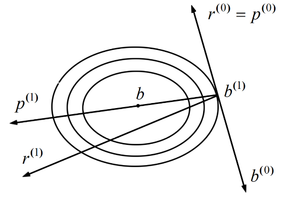
|
| Figure 3. Graphical representation of the Conjugated Gradient method |
Supposing there is an initial estimate , according to the Gradient method, one can start from this point and research the minimum of , across the direction , obtaining . Observing Figure 3, it can be verified that the best progression of would not be the more inclined direction, but the direction which points to the center of the ellipse.
In fact, the new minimizing point would coincide with the exact solution of b, and thus the iterative process would end with just two iterations. Therefore a direction can be chosen as:
|
(36) |
As it can be observed, complying with the orthogonality of the successive residues verified previously, there is
|
(37) |
in such a way that
|
(38) |
The sought directions are
|
(39) |
where is given by
|
(40) |
The iterations of the CG method satisfy the following error estimate [7]:
|
(41) |
where .
Thus, it can be noticed that the CG method, theoretically, calculates the exact solution in n iterations, which is not verified in practice due to the application of this method in finite precision arithmetic’s and the introduction of rounding errors which destroy the exact conjugacy of the direction and the exact orthogonality of the residues . Thus, this method takes a typical iterative form.
One way to make this iterative method faster consists in transforming the system into an equivalent system, where the matrix has a more favorable conditioning number. According to Eq. (41), if it is possible to reduce , consequently a fast convergence is achieved.
The transformation of the pre- and post-multiplication of the matrix A by the matrixes P and Q being invertible by the following manner:
|
(42) |
The system now corresponds, therefore, to , with , and , the matrixes P and Q having to be chosen in the way that provides the best convergence properties to the matrix in relation to the original matrix A. This procedure is known as preconditioning of the original equations system, P and Q being known by the name of preconditioning matrixes.
Considering that in the CG method the transformed matrix has to keep being a symmetric positive definite matrix, the preconditioning will also have to preserve this property. In fact, it can be obtained making and , and in this manner, it can be concluded that , , and .
Thus, it can be verified that On the other hand, choosing there is the relation also being valid, with
|
|
(43) |
and
|
(44) |
From that, there is:
|
(45) |
|
(46) |
|
(47) |
|
|
(48) |
and
|
(49) |
keeping these expressions for the following iterations.
Algorithm 2 presents the preconditioned CG method (PCG), where it can be noticed that at each iteration it is necessary to solve the auxiliary system:
|
(50) |
and it is desirable that its resolution is not very laborious.
| Start |
| Read A, f |
| Estimate b(0) |
| Determine a tolerance γ |
| Calculate |
| Solve |
| Attribute |
| For j = 0, 1, ... until convergence |
| Solve |
| End |
| End |
4.3 Incomplete LU decomposition (ILU)
The incomplete LU decomposition (ILU) consists in decomposing a matrix A in an incomplete manner, as the name suggests. Such decomposition is in the A = LU – R form, where L and U are, respectively, inferior and superior triangular matrixes A and R represents the residue or decomposition error. On the matrix R, conditions are imposed such as having null terms in determined positions in order to maintain certain characteristics of the original matrix A.
A general algorithm for ILU can be obtained applying the Gaussian Elimination [7] and having some elements in predetermined positions. For this, a set of points is determined where the elements of the matrix will be null. In this case, there can be several variations of the ILU decomposition, for example: ILU(0), where the structure of the LU decomposition is identical to the structure of matrix A, that is, it does not allow extra fillings; ILU(1), where the filling of one additional diagonal is allowed in each LU factor, etc. In this paper, ILU(1) was chosen, which will be called 7-points ILU (since the stencil of the original problem has 5 points).
Thus, given the incomplete LU decomposition, it is solved in an iterative process composed of the following steps:
(1) to obtain , being the residue vector
(2) to obtain .
Thus, the solution in the iteration k +1 is such that:
|
(51) |
4.4 Multigrid method (MG)
The MG method [5,6,32] makes use of the error smoothing characteristics from the classic iterative methods: it occurs fast (in the initial iterations) for oscillatory components, while for smooth components, for a high number of iterations, such methods lose their efficiency. Thus, the MG method works with a system of auxiliary coarser grids (with a lower number of points) in which the error components are quickly smoothed, in order to return to the original grid. The information is transferred between grids through operators, called restriction operators (information from a fine to a following coarser grid), generically represented by and defined by
|
(52) |
or prolongation ones (information from the coarse grid to a finer one), represented generically by and defined by
|
(53) |
The restriction operator applied in this paper was the complete weighting operator and the prolongation operator was the bilinear interpolation [5,6,32,33].
In this paper, moreover, the V-Cycle was applied, for its computational efficiency. The equations of Poisson and Reaction-Diffusion being linear, the correction scheme (CS) was applied, which transfers only the residues to the coarser grids [5,6]. The coarsening ratio, considering uniform grids, is defined as r = H/h, where h represents the size of the spacing of the fine grid, , (also called the dimension of the fine grid elements), and H the size at the element of the next coarser grid, .
Figure 4 illustrates the cycle-V with CS for five grids. The superscripts h, 2h , 4h, ... indicate the grid where the vectors and matrixes are defined, the smoothing numbers (S) being achieved in the restriction process (R) (pre-smoothing) and prolongation (P) (post-smoothing) being represented, respectively, by and .
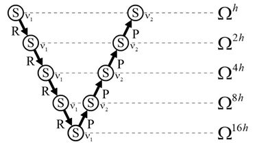
|
| Figure 4. Cycle-V for five grids |
In this paper, the MG with GS and ILU solvers was applied. Such iterative methods were also applied as preconditioners for the PCG method, that is, they were used to solve the linear system given by Eq. (50) at each iteration of the CG method.
5. Results
5.1 Methodology and computational details
Computational tests were done to calculate the values of p, u and v in the discretized model problem, Eqs. (22) and (25), applying the following methodology:
- 1) Multigrid with Gauss-Seidel solver (MG-GS).
- 2) Multigrid with ILU solver (MG-ILU).
- 3) Preconditioned Conjugated Gradient with Multigrid and Gauss-Seidel solver (PCG-MG-GS).
- 4) Preconditioned Conjugated Gradient with Multigrid and ILU solver (PCG-MG-ILU).
In all simulations and for all the variables of interest, the stop criterion applied was the nondimensionalized residue -norm based on the initial estimate, given by:
|
(54) |
where is the residue on the current iteration, is the residue of the initial estimate, and ε is the tolerance.
In this paper the null vector was utilized as the initial estimate for all the variables of interest and with the use of double precision. The standard coarsening ratio was utilized, that is , [5], where the Multigrid method started from the finest grid and got to the coarsest grid possible, that is, the grid with volumes. The number of unknowns in the finest grids was: 16, 3232, 6464, 128128, 256256, 512512 and 10241024. The number of pre- and post-smoothing was equals to .
The computer utilized for the simulations has an Intel Core i7-5500 processor, a 2.40 Ghz CPU, 16.0 Gb memory and a 64 bits Windows 10 operational system.
Four parameters were analyzed in order to compare the four methodologies:
- -norm for numerical error ();
- -norm for nondimensionalized residue based on the initial estimate (Eq. (54));
- Empirical convergence factor, defined as [6]:
|
|
(55) |
and
- CPU time.
5.2 Analysis of the pressure
This phase it is intended to determine the best method to solve the Poisson equation, which models pressure, determining a method to solve the velocities equations. In this case, MG-GS, MG-ILU, PCG-MG-GS and PCG-MG-ILU were utilized for pressure and MG-GS for the velocities.
The behavior of the -norm was initially evaluated for the four studied methods, where it could be noticed that all of them presented a reduction in the numerical error norm with the increase in the size of the problem; a desirable characteristic in a convergent numerical method (Figure 5).
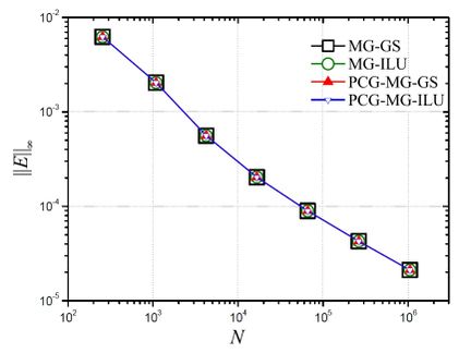
|
| Figure 5. -norm for the numerical error () versus size of problem (N) for p |
Figure 6 presents the number of iterations necessary in order to reach the stop criterion for the problem with . Based on this figure, it can be noticed that PCG-MG-ILU reached the stop criterion in a lower number of iterations.
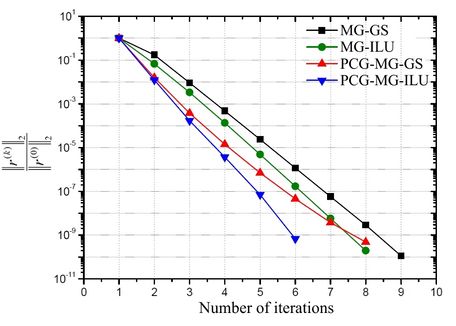
|
| Figure 6. -norm for the nondimensionalized residue by the norm of initial estimate versus number of
iterations for the problem with for p |
Figure 7 illustrates the behavior of the empirical convergence factor with the increase of the size of the problem. Based on this figure, it can be claimed again that the PCG-MG-ILU methodology presented the best results, since it is the one that generated the best values for the convergence factors, that is, values near to zero [5,34].
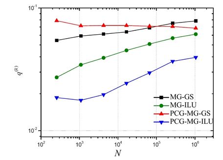
|
| Figure 7. Empirical convergence factor () versus size of the problem (N) for p |
Figure 8 illustrates the behavior of the CPU time (in seconds) of the simulations with the increase of the size of the problem. It can be noticed that the computational times became very close, with a slight advantage for the PCG-MG-ILU methodology, which can be confirmed in sequence.
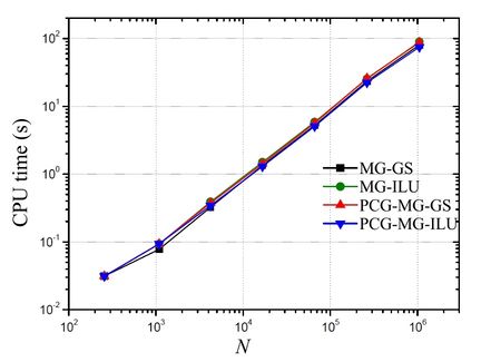
|
| Figure 8. CPU time (in seconds) versus size of the problem (N) for p |
The speed-up is a measure utilized to determine the increase in velocity obtained during the execution of a program utilizing an algorithm “A” in relation to its execution utilizing an algorithm “B” [6]. It is given by:
|
(56) |
Table 1 shows the Speed-up of the three methods MG-GS, MG-ILU and PCG-MG-GS in relation to the PCG-MG-ILU method.
| N | MG-GS | MG-ILU | PCG-MG-GS |
|---|---|---|---|
| 1616 | 1 | 1 | 1 |
| 3232 | 0.833 | 1 | 1 |
| 6464 | 0.948 | 1.136 | 1.109 |
| 128128 | 1.036 | 1.156 | 1.109 |
| 256256 | 1.033 | 1.153 | 1.110 |
| 512512 | 1.055 | 1.139 | 1.160 |
| 10241024 | 1.074 | 1.194 | 1.167 |
According to the data presented in this table, it can be confirmed that the CPU times are close among themselves, but there is a slight advantage with the use of PCG-MG-ILU (Speed-up above 1), as described in [35].
It all leads us to conclude that the CGP-MG-ILU method has the potential to accelerate the convergence of the presented problem.
5.3 Analysis of the velocities
In this phase, it is intended to determine the best method to solve the Reaction-Diffusion equations, which model the velocities u and v, determining the best method for pressure presented in the previous section, which was PCG-MG-ILU. Since the results for the velocities u and v for all the parameters are similar, it was chose to display only the results for u.
Figure 9 shows the behavior of the numerical error versus the size of the problem, for the several solution methods. It can be noticed that the four studied methods presented an expected characteristic for the convergent iterative methods, that is, the decrease in the numerical error with the increase in the size of the problem. It can also be noticed that the presented error have values which are very close among themselves.
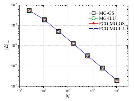
|
| Figure 9. -norm for the numerical error () versus size of the problem (N) for p |
Figure 10 displays the behavior of -norm of the nondimensionalized residue by -norm of the initial estimate in function of the number of iterations for the problem with volumes. Based on this figure, it can be noticed that the PCG-MG-ILU and the MG-ILU methods were the ones which achieved the stop criterion in the lowest number of iterations.
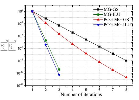
|
| Figure 10. -norm for the nondimensionalized residue by -norm of the initial estimate versus number of iterations for the problem with for u |
Figure 11 illustrates the behavior of the empirical convergence factor in function of the size of the problem. Based on this figure, it can be concluded that the PCG-MG-ILU method presented the best results, since it generated the best values for the convergence factors (closest values to zero), besides decreasing its value with the increase of the size of the problem.
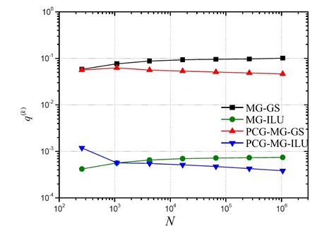
|
| Figure 11. Empirical convergence factor () versus size of the problem (N) for u |
Figure 12 shows the CPU times (in seconds) of the simulations with the increase of the size of the problem. Based on this figure, it can be noticed that the computational times were very close, with a slight advantage for the PCG-MG-ILU methodology, which can be confirmed in the results presented in the sequence.
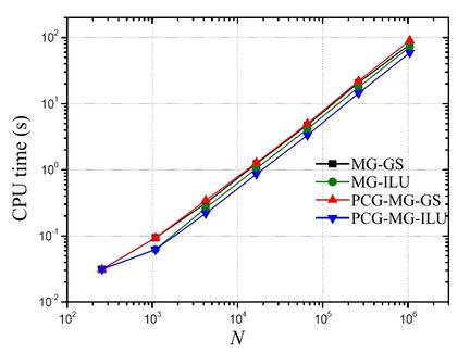
|
| Figure 12. CPU time (in seconds) versus size of the problem (N) |
Table 2 presents the Speed-up (Eq.(56)) of the MG-GS, MG-ILU and PCG-MG-GS methods in relation to the PCG-MG-ILU method. In this table, it can be confirmed that the CPU times are close among themselves, but there is an advantage with the use of PCG-MG-ILU, that is, the method that most accelerated the convergence of the iterative process for the presented problem.
| N | MG-GS | MG-ILU | PCG-MG-GS |
|---|---|---|---|
| 1616 | 1 | 1 | 1 |
| 3232 | 1.5 | 1 | 1.5 |
| 6464 | 1.428 | 1.214 | 1.571 |
| 128128 | 1.436 | 1.218 | 1.490 |
| 256256 | 1.425 | 1.242 | 1.495 |
| 512512 | 1.443 | 1.230 | 1.524 |
| 10241024 | 1.337 | 1.228 | 1.535 |
5.4 Algorithm
After the tests of the two previous phases (sections 5.2 and 5.3), whose objective was to identify the best methods for the solution of the equations for the variables (Poisson equation) and and (Reaction-Diffusion equations), we get to the point where the best methods were applied simultaneously to solve the Navier-Stokes equations.
The results presented below are compared the classic Gauss-Seidel (GS) method in its singlegrid version (only grid method) so that the gains can be measured when using the proposed algorithm (adaptation of the Projection method presented in Algorithm 1), that is, using the PCG-MG-ILU solver in the solution of the linear systems given in steps 1 and 2 of Algorithm 1.
Figure 13 presents the behavior of -norm of the nondimensionalized residue by the initial estimate in function of the number of iterations for the problem with volumes for the variables , and . Based on this figure, it can be noticed that the PCG-MG-ILU method reached the stop criterion ε = 10–10 in an extremely lower number of iterations, both for and for and .
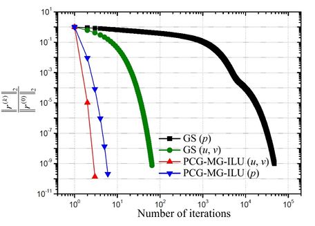
|
| Figure 13. -norm of the nondimensionalized residue by norm for the initial estimate versus number of iterations for the problem with for , and |
Figure 14 illustrates the behavior of the empirical convergence factor with the increase of the size of the problem. Based on this figure, it can be concluded that the PCG-MG-ILU method presented much better results for the convergence factors for the three variables of interest, comparing with the classic GS method.
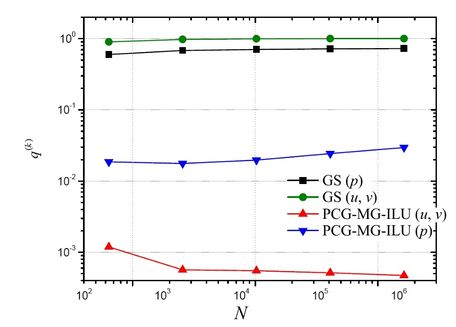
|
| Figure 14. Empirical convergence factor () versus size of the problem (N) for , and |
Figure 15 contains the values of the CPU times (in seconds) of the simulations with the increase of the size of the problem. Based on this figure, it can be noticed that the PCG-MG-ILU methodology was the one that converged faster, being quite evident the difference in CPU time between the proposed methodology and the classic GS method.
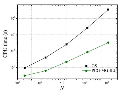
|
| Figure 15. CPU time (in seconds) versus size of the problem (N) |
Table 3 presents the Speed-up (Eq.(56)) on the GS method in relation to the PCG-MG-ILU method. According to the data on this table, the methodology that uses the PCG-MG-ILU method proved much more efficient than the methodology that utilizes the GS method, reaching a 105 times higher velocity for the biggest problem compared in this table. It can also be noticed that the Speed-up increases as the size of the problem increases, which is a highly desirable property.
| N | SP |
|---|---|
| 88 | 3.013 |
| 1616 | 6.504 |
| 3232 | 11.785 |
| 6464 | 31.181 |
| 128128 | 105.242 |
Another complementary study can be done through the comparative of complexities of algorithms utilizing the different methods. For complexity analysis of such algorithms, the exponent p was calculated; obtaining the by least square fitting, for the function given by
|
(57) |
where p represents the order of the solver associated with the employed method and c is a coefficient that depends on each method and each solver, N is the number of unknowns of the system and the CPU time.
For the ideal MG method, , meaning that the computational effort increases linearly with the size of the grid [3,6]. Thus, for a given hardware and compilator, the closer p is to the unity, the more efficient the algorithm is and the lower the value of c, the faster it is.
Table 4 presents the values of p and c for the curve adjustments obtained for the studied methods (data from Figure 15). In this table, it can be observed that the value of for PCG-MG-ILU, being for GS, as expected from literature [6]. Besides that, the lower value for c appears for PCG-MG-ILU.
| Metodology | c | p |
|---|---|---|
| GS | 5.332E-04 | 1.855 |
| PCG-MG-ILU | 4.272E-05 | 0.984 |
6. Conclusion
In this paper, a problem of a two dimensional laminar flow of an incompressible, isothermal fluid in a transient regime given by the Navier-Stokes equations was solved utilizing a Projection method with the intention of obtaining the primary variables u, v, and p. The Finite Volume Method in staggered grids in the discretization process was used, generating systems of linear equations, which were solved by applying the Geometric Multigrid method and some combinations with different solvers. Numerical tests were performed for the Taylor-Green vortices problems, which have a known analytical solution. Based on the obtained results, it was verified that the proposed algorithm, the algorithm that contemplates the PCG-MG-ILU method on the solution systems arising from pressure and velocities, presented results better than the methodologies compared in this paper, since it converges with few iterations, has the best empirical convergence factor, Speed-up and complexity factors values. Therefore, the computational time was reduced, for example, in up to 105 times for the problem with 128128 in relation to a classic method, and an improvement tendency of this factor (Speed-up) was noticed with the increase of the size of the problem, a quite desirable property.
Acknowledgements
The authors would like to thank the Graduate Program in Numerical Methods in Engineering (PPGMNE) of the Federal University of Paraná (Brazil). The third author thanks the scholarship of Meteorological System of Paraná (SIMEPAR). This study was financied partly by the Coordenação de Aperfeiçoamento de Pessoal de Nível Superior - Brasil (CAPES) - Finance Code 001.
References
[1] Mitin A.V. Linear extrapolation in an iterative method for solving systems of equations, U.S.S.R. Comput. Maths. Math. Phys., 25(2):1-6, 1985.
[2] Fedorenko R.P. On the speed of convergence of an iteration process. U.S.S.R. Comput. Math. And Math. Phys., 4(3):227-235, 1964.
[3] Brandt A. Multi-level adaptive solutions to boundary-value problems. Mathematics of Computation, 31:333-390, 1977.
[4] Pletcher R., Tannehill J., Anderson D. Computational fluid mechanics and heat transfer. Series in Computational and Physical processes in Mechanics and Thermal Sciences, 2nd ed., Taylor & Francis, 1997.
[5] Briggs W.L., Henson V.E., McCormick S.F. A multigrid tutorial. 2nd ed., SIAM, 2000.
[6] Trottenberg U., Oosterlee C., Schüller A. Multigrid. Academic Press, 2001.
[7] Saad Y. Iterative methods for sparse linear systems. SIAM, 2003.
[8] Batchelor G. An introduction to fluid dynamics. Cambridge University Press, 1970.
[9] Peyret R., Taylor T.D. Computational methods for fluids flow. Springer-Verlag, 1983.
[10] Panton R.L. Incompressible flow. John Wiley & Sons, 1984.
[11] Fletcher C.A.J. Computational methods for fluid dynamics. Vol. 1, 2nd ed., Springer, 1992.
[12] Maliska C.R. Transferência de calor e mecânica dos fluidos computacional. 2nd ed., LTC, 2004.
[13] Ferziger J.H., Peric M. Computational methods for fluid dynamics. Springer-Verlag, 2002.
[14] Guermond J.L., Minev P., Shen J. An overview of projection methods for incompressible flows. Computer Methods in Applied Mechanics and Engineering, 195(44):6011-6045, 2006.
[15] Griffith B.E. An accurate and efficient method for the incompressible Navier–Stokes equations using the projection method as a preconditioner. Journal of Computational Physics, 228(20):7565-7595, 2009.
[16] Kim J., Moin P. Application of a fractional-step method to incompressible Navier Stokes equations. Journal of Computational Physics, 59:308-323, 1985.
[17] Hughes W.F., Brighton J.A. Dinâmica dos fluidos. McGraw Hill, 1967.
[18] Pearson C.E. A computational method for time dependent two dimensional incompressible viscous flow problems. Sperry-Rand Research Center, 1964.
[19] Ernst O.G., Gander M.J. Why it is difficult to solve Helmholtz problems with classical iterative methods? Computational Science and Engineering, 83:325-363, 2012.
[20] Incropera F.P., Dewitt D.P. Bergman T.L., Lavine, A.S. Fundamentals of heat and mass transfer. 6 ed., John Wiley & Sons, 2007.
[21] Harlow F.H., Welch J.E. Numerical calculation of time-dependent viscous incompressible flow of fluid with free surface. The Physics of Fluids, 8:2182-2189, 1965.
[22] Shih T.M., Tan C.H., Hwang B.C. Effects of grid staggering on numerical scheme. Int. J. Num. Met. Fluids, 9:193-212, 1989.
[23] Devendran D., Corona E. Projection nethods, computational fluid dynamics reading group. Courant Institute of Mathematical Sciences of New York University, New York, 2009.
[24] Chorin A.J. Numerical solution of the Navier-Stokes equations. Mathematics of Computation, 22(104):745-762, 1968.
[25] Temam R. Sur l’approximation de la solution des équations de Navier-Stokes par la méthode des fractionnaires. Archive for Rational Mechanics and Analysis, 33(5):377-385, 1969.
[26] Goda K. A multistep technique with implicit difference schemes for calculating two-or three-dimensional cavity flows. Journal of Computational Physics, 30(1):76-95, 1979.
[27] Van Kan J. A second-order accurate pressure-correction scheme for viscous incompressible flow. SIAM J. Sci. Stat. Comput., 7(3):870-891, 1986.
[28] Timmemans L.J.P., Minev P.D., Van de Vosse F.N. An approximate projection scheme for incompressible flow using spectral elements. International Journal for Numerical Methods in Fluids, 22(7):673-688, 1996.
[29] Guermond J.L., Shen J. On the error estimates for the rotational pressure-correction projection methods. Math. Comput., 73(248):1719–1737, 2004.
[30] Kalland K.A. Navier-stokes solver for single and two-phase flow. Master Thesis, University of Oslo, 2008.
[31] Villar M.M. Análise numérica detalhada de escoamentos multifásicos bidimensionais. Thesis UFU, Uberlandia, Brazil, 2007.
[32] Wesseling P. An introduction to multigrid methods. John Wiley & Sons, 1992.
[33] Hackbush W. Multigrid methods and applications. Springer-Verlag, 1985.
[34] Burden R.L., Faires J.D. Análise numérica. Pioneira Thomson Learning, 2007.
[35] Anunciação M.A.M., Pinto M.A.V., Neundorf R.L. Análise de parâmetros do método do Gradiente Conjugado pré-condicionado com Multigrid para a equação de Poisson bidimensional. In XXXVIII Ibero-Latin American Congress on Computational Methods in Engineering (CILAMCE), Proceedings Florianópolis, 2017.
Document information
Published on 10/03/20
Accepted on 25/12/19
Submitted on 13/06/19
Volume 36, Issue 1, 2020
DOI: 10.23967/j.rimni.2020.01.003
Licence: CC BY-NC-SA license
