(Created page with "<!-- metadata commented in wiki content <div class="center" style="width: auto; margin-left: auto; margin-right: auto;"> <big>Analysis of Short-Circuit Failures in Synchrono...") |
m (Arm1987 moved page Arrieta et al 2020a to Arrieta et al 2020b) |
||
| (46 intermediate revisions by 3 users not shown) | |||
| Line 6: | Line 6: | ||
<div class="center" style="width: auto; margin-left: auto; margin-right: auto;"> | <div class="center" style="width: auto; margin-left: auto; margin-right: auto;"> | ||
| − | <big>Edgardo Arrieta<sup>1</sup>, Neider Romero<sup>2</sup>, Melissa Torregroza<sup>3</sup>, | + | <big>Edgardo Arrieta<sup>1</sup>, Neider Romero<sup>2</sup>, Melissa Torregroza<sup>3</sup>, Isaías Fuly<sup>1</sup></div> |
<div class="center" style="width: auto; margin-left: auto; margin-right: auto;"> | <div class="center" style="width: auto; margin-left: auto; margin-right: auto;"> | ||
| Line 17: | Line 17: | ||
<sup>3</sup> CERin, Department Electric Engineering, Universidade Federal de Itajubá, Itajubá, Brasil.</div> | <sup>3</sup> CERin, Department Electric Engineering, Universidade Federal de Itajubá, Itajubá, Brasil.</div> | ||
| − | |||
| − | |||
--> | --> | ||
| − | + | ==Abstract== | |
| − | + | ||
In this paper, a mathematical model using finite element software is developed. An electromagnetic analysis is performed to determine the behavior of quantities such as magnetic flux density and output voltage when short-circuit failures occur in the winding of the rotor poles of a synchronous small size machine when it works as a generator. The voltage values obtained from the simulations were compared with data from actual tests performed in the laboratory. | In this paper, a mathematical model using finite element software is developed. An electromagnetic analysis is performed to determine the behavior of quantities such as magnetic flux density and output voltage when short-circuit failures occur in the winding of the rotor poles of a synchronous small size machine when it works as a generator. The voltage values obtained from the simulations were compared with data from actual tests performed in the laboratory. | ||
| − | '''Keywords''': Synchronous machine, finite elements, magnetic flux, short-circuit | + | '''Keywords''': Synchronous machine, finite elements, magnetic flux, short-circuit |
| − | =1. | + | ==1. Introduction== |
A synchronous machine (SM) is an electric machine capable of generating electrical energy through the transformation of mechanical energy present in its rotation axle [1,2]. The importance of the synchronous machine within the electricity generation system makes it essential to maintain its reliability and performance to avoid failures that may affect it and also the electricity generation and transmission system. | A synchronous machine (SM) is an electric machine capable of generating electrical energy through the transformation of mechanical energy present in its rotation axle [1,2]. The importance of the synchronous machine within the electricity generation system makes it essential to maintain its reliability and performance to avoid failures that may affect it and also the electricity generation and transmission system. | ||
| Line 37: | Line 34: | ||
This work has as main objective the use of the finite element method to present an analysis of the behavior of the magnetic flux density when short circuit failures occur in the windings of the rotor poles of a small synchronous machine, and when it works under different operating conditions. | This work has as main objective the use of the finite element method to present an analysis of the behavior of the magnetic flux density when short circuit failures occur in the windings of the rotor poles of a small synchronous machine, and when it works under different operating conditions. | ||
| − | =2. | + | ==2. Finite elements== |
The Finite Element Method also known as FEM is a tool widely used to solve engineering and physics problems, especially for the study of electromagnetic phenomena where it has taken a lot of recognition in recent years. This is due to the high degree of accuracy that this method is capable of achieving, as well as its capacity for modeling complex systems [5,6]. Therefore, the Finite Element Method allows us to solve, on a large scale, the complex problem of electromagnetic field, planted through simple and general data structures [7,8]. | The Finite Element Method also known as FEM is a tool widely used to solve engineering and physics problems, especially for the study of electromagnetic phenomena where it has taken a lot of recognition in recent years. This is due to the high degree of accuracy that this method is capable of achieving, as well as its capacity for modeling complex systems [5,6]. Therefore, the Finite Element Method allows us to solve, on a large scale, the complex problem of electromagnetic field, planted through simple and general data structures [7,8]. | ||
| Line 43: | Line 40: | ||
FEM is a method of approximating continuous problems that are divided into a finite number of parts, called finite elements. The behavior of these small parts is specified through a finite number of parameters associated with the nodes, which are a series of points that connect the elements to each other. The behavior in each element is defined by a matrix which is formed by a group of polynomial functions that depend on the interpolation of known values in the nodes. The process of dividing the discrete geometric model into small finite elements is called a mesh [9,10]. The division of the geometric model into triangular elements is widely used, specifically in the analysis of magnetic devices because mathematically they are easy to understand, their results are quite approximate, and they have a lower computational cost [11]. | FEM is a method of approximating continuous problems that are divided into a finite number of parts, called finite elements. The behavior of these small parts is specified through a finite number of parameters associated with the nodes, which are a series of points that connect the elements to each other. The behavior in each element is defined by a matrix which is formed by a group of polynomial functions that depend on the interpolation of known values in the nodes. The process of dividing the discrete geometric model into small finite elements is called a mesh [9,10]. The division of the geometric model into triangular elements is widely used, specifically in the analysis of magnetic devices because mathematically they are easy to understand, their results are quite approximate, and they have a lower computational cost [11]. | ||
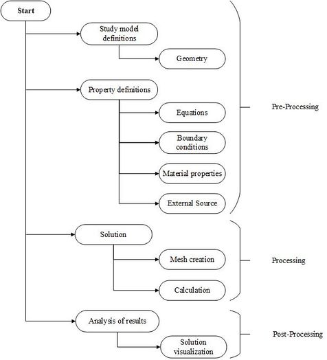
| − | To solve a physical problem using finite element software, the steps that are represented in the flow diagram of Figure 1 are performed. In that graphic we present a general solution of how the finite element software finds the solution for the continuous medium model. The process for determining the model solution is divided into four stages, the first one is the Pre-processing stage, in this phase we have the definition of the model in which the geometry of the medium will be defined. Then, in the second one, we have the Property Definitions where the equations, boundary conditions, material properties and external source are defined. The equations are specified depending on the type of analysis (static or dynamic) and Maxwell's laws used for the study (Ampere, Faraday, Gauss). Boundary conditions are the boundaries that limit the region of the solution. In the properties of the materials, the materials that make up the physical environment are defined, these can be obtained from the software libraries. The external source is the excitation source of the model that in this case is the density of the external current. | + | To solve a physical problem using finite element software, the steps that are represented in the flow diagram of [[#img-1|Figure 1]] are performed. In that graphic we present a general solution of how the finite element software finds the solution for the continuous medium model. The process for determining the model solution is divided into four stages, the first one is the Pre-processing stage, in this phase we have the definition of the model in which the geometry of the medium will be defined. Then, in the second one, we have the Property Definitions where the equations, boundary conditions, material properties and external source are defined. The equations are specified depending on the type of analysis (static or dynamic) and Maxwell's laws used for the study (Ampere, Faraday, Gauss). Boundary conditions are the boundaries that limit the region of the solution. In the properties of the materials, the materials that make up the physical environment are defined, these can be obtained from the software libraries. The external source is the excitation source of the model that in this case is the density of the external current. |
The third phase is the solution, this is part of the processing step, here the mesh of the discrete system is created and also during the calculation of the equations that make up the discrete system, the quantities of interest are determined, which in our specific case is the magnetic flux density. | The third phase is the solution, this is part of the processing step, here the mesh of the discrete system is created and also during the calculation of the equations that make up the discrete system, the quantities of interest are determined, which in our specific case is the magnetic flux density. | ||
| Line 49: | Line 46: | ||
Finally, we have the fourth and last one phase, the post-processed, in this step the results of the simulation are graphically represented to make the analysis of the results, it is also allowed to export the results to be analyzed in other software. | Finally, we have the fourth and last one phase, the post-processed, in this step the results of the simulation are graphically represented to make the analysis of the results, it is also allowed to export the results to be analyzed in other software. | ||
| − | <div | + | <div id='img-1'></div> |
| − | [[Image:Draft_Arrieta_886506833-image1.jpeg| | + | {| style="text-align: center; border: 1px solid #BBB; margin: 1em auto; width: auto;max-width: auto;" |
| + | |- | ||
| + | |style="padding:10px;"| [[Image:Draft_Arrieta_886506833-image1.jpeg|476px]] | ||
| + | |- style="text-align: center; font-size: 75%;" | ||
| + | | colspan="1" style="padding-bottom:10px;"| '''Figure 1'''. Flow diagram for calculation with FEM software | ||
| + | |} | ||
| − | + | ==3. Methodology== | |
| − | + | ||
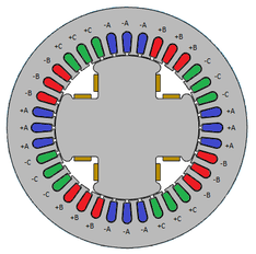
| − | + | This project uses a model for a small machine. The geometric model of the machine is based on a machine that has 4 poles and 36 slots in the stator, and an external diameter of the stator is 0.5 meters. The electrical characteristics in nominal conditions are shown in [[#tab-1|Tables 1]], [[#tab-2|2]] and in [[#img-2|Figure 2]], a main section of the geometric model that represents this machine is shown. | |
| − | + | <div class="center" style="font-size: 75%;">'''Table 1'''. Small SM electrical characteristics</div> | |
| − | <div | + | <div id='tab-1'></div> |
| − | + | {| class="wikitable" style="margin: 1em auto 0.1em auto;border-collapse: collapse;font-size:85%;width:auto;" | |
| − | + | |-style="text-align:center" | |
| − | {| style=" | + | ! Number of<br/>phases !! Nominal<br/>power !! Nominal<br/>voltage !! Nominal<br/>current !! Power<br/>factor !! Nominal<br/>speed !! style="vertical-align:top" |Frequency<br/> |
| − | + | ||
| − | + | ||
| − | + | ||
| − | |- | + | |
| − | + | ||
| − | + | ||
| − | + | ||
| − | + | ||
| − | + | ||
| − | + | ||
| − | + | ||
| − | + | ||
| − | + | ||
| − | + | ||
| − | + | ||
| − | + | ||
| − | + | ||
| − | + | ||
|- | |- | ||
| − | | style=" | + | | style="text-align: center;"|3 |
| − | | style=" | + | | style="text-align: center;vertical-align: top;"|35 KVA |
| + | | style="text-align: center;vertical-align: top;"|VFF=380 [V]/<br/>VFN=220[V] | ||
| + | | style="text-align: center;vertical-align: top;"|53.2 [A] | ||
| + | | style="text-align: center;vertical-align: top;"|<math>\cos \phi=0.8</math> | ||
| + | | style="text-align: center;vertical-align: top;"|1800 [rpm] | ||
| + | | style="text-align: center;vertical-align: top;"|60 [Hz] | ||
|} | |} | ||
| − | The resistors for the stator circuit and the rotor excitation were obtained through manual measurements of the real synchronous machine and are presented in | + | The resistors for the stator circuit and the rotor excitation were obtained through manual measurements of the real synchronous machine and are presented in [[#tab-2|Table 2]]. |
| − | <div class="center" style=" | + | <div class="center" style="font-size: 75%;">'''Table 2'''. Resistances</div> |
| − | '''Table 2'''. Resistances | + | |
| − | {| style="margin: 1em auto 0.1em auto;border-collapse: collapse;" | + | <div id='tab-2'></div> |
| + | {| class="wikitable" style="margin: 1em auto 0.1em auto;border-collapse: collapse;font-size:85%;width:auto;" | ||
| + | |-style="text-align:center" | ||
| + | ! Stator !! Rotor | ||
|- | |- | ||
| − | | style=" | + | | style="text-align: center;vertical-align: top;"|0.3 <math>[\Omega ]</math> /phase |
| − | + | | style="text-align: center;vertical-align: top;"|15 <math>[\Omega ]</math> | |
| − | + | ||
| − | + | ||
| − | | style=" | + | |
|} | |} | ||
| − | <div | + | <div id='img-2'></div> |
| − | + | {| style="text-align: center; border: 1px solid #BBB; margin: 1em auto; width: auto;max-width: auto;" | |
| + | |- | ||
| + | |style="padding:10px;"| [[Image:Draft_Arrieta_886506833-image2.png|234px]] | ||
| + | |- style="text-align: center; font-size: 75%;" | ||
| + | | colspan="1" style="padding-bottom:10px;"| '''Figure 2'''. Cross Section of SM | ||
| + | |} | ||
| − | |||
| − | |||
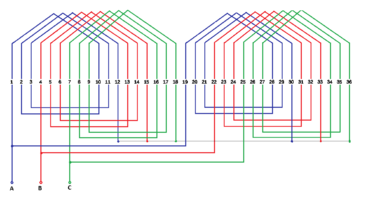
| − | In | + | In [[#img-2|Figure 2]] it is shown the machine's stator winding, here the phases are represented by the letters A, B and C. The positive sign indicates that the coil goes up through the stator in the indicated slot, while the negative sign indicates that it is going down through that slot, as shown in [[#img-3|Figure 3]]. |
| − | <div | + | <div id='img-3'></div> |
| − | + | {| style="text-align: center; border: 1px solid #BBB; margin: 1em auto; width: auto;max-width: auto;" | |
| + | |- | ||
| + | |style="padding:10px;"| [[Image:Draft_Arrieta_886506833-image3.png|366px]] | ||
| + | |- style="text-align: center; font-size: 75%;" | ||
| + | | colspan="1" style="padding-bottom:10px;"| '''Figure 3'''. Diagram of the winding of the SM | ||
| + | |} | ||
| − | + | ==4. Results== | |
| − | + | ||
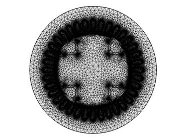
| − | + | [[#img-4|Figure 4]] shows the geometric model of the synchronous machine after the mesh process. The mesh is made up of a set of 51 417 triangular elements. The size of the triangular elements was automatically defined by the software, in the figure it can be seen that in the most critical areas of the geometric model the triangular elements are thinner so that the results of the simulation are more accurate. | |
| − | + | <div id='img-4'></div> | |
| + | {| style="text-align: center; border: 1px solid #BBB; margin: 1em auto; width: auto;max-width: auto;" | ||
| + | |- | ||
| + | |style="padding:10px;"| [[Image:Draft_Arrieta_886506833-image4.jpeg|370px]] | ||
| + | |- style="text-align: center; font-size: 75%;" | ||
| + | | colspan="1" style="padding-bottom:10px;"| '''Figure 4'''. Mesh SM | ||
| + | |} | ||
| − | |||
| − | |||
| − | + | ===4.1 Analysis under normal operating conditions and with no load connected=== | |
| − | + | ||
| − | + | The simulations were made as a function of time and the materials were soft iron for the rotor core and the stator, air for the air gap and copper for the windings. From the simulation under normal operating conditions, [[#img-5|Figure 5]] was obtained, showing the magnetic flux density on the surface of the SM, the magnetic flux density is measured in Tesla [T]. | |
| − | + | <div id='img-5'></div> | |
| + | {| style="text-align: center; border: 1px solid #BBB; margin: 1em auto; width: auto;max-width: auto;" | ||
| + | |- | ||
| + | |style="padding:10px;"| [[Image:Draft_Arrieta_886506833-image5.png|300px]] | ||
| + | |- style="text-align: center; font-size: 75%;" | ||
| + | | colspan="1" style="padding:10px;"| '''Figure 5'''. Magnetic flow density of SM in normal conditions | ||
| + | |} | ||
| − | |||
| − | |||
| − | + | In [[#img-5|Figure 5]], it can be seen that the magnetic flux density has rotational symmetry that is maintained throughout the operation time. In addition, it is also observed how the magnetic paths are established, they leave a north pole and go to a south pole, in this way, they pass through the teeth and the stator crown. When the magnetic flux density passes through the teeth of the stator it becomes more concentrated due to the reduction in the available area since the normal pitch of the magnetic flux density is restricted, as shown in [[#img-6|Figure 6]]. The highest density of magnetic flux within the SM is concentrated in the corners that join the rotor poles, and in this case, it has a value of <math>0.88 [T]</math> and the minimum value of the magnetic flux density is around <math>80 [\mu T]</math>. In the stator teeth, the flow density reaches a maximum value of <math>0.53 [T]</math> when in front of them are one of the poles of the rotor and a minimum value of <math>110 [\mu T]</math> when in front of them passes the space between two poles. In [[#tab-3|Table 3]], we can find other values of the magnetic flux density on the surface of the SM, where it is shown that the magnetic flux density is constant in each of the poles and in [[#img-7|Figure 7]] it shows the behavior of the magnetic flux in the air gap. | |
| − | + | ||
| − | + | <div id='img-6'></div> | |
| + | {| style="text-align: center; border: 1px solid #BBB; margin: 1em auto; width: auto;max-width: auto;" | ||
| + | |- | ||
| + | |style="padding:10px;"| [[Image:Draft_Arrieta_886506833-image6.png|290px]] | ||
| + | |- style="text-align: center; font-size: 75%;" | ||
| + | | colspan="1" style="padding:10px;"| '''Figure 6'''. Magnetic flow density concentration in the stator teeth | ||
| + | |} | ||
| − | |||
| − | |||
| − | <div class="center" style=" | + | <div class="center" style="font-size: 75%;">'''Table 3'''. Density values of magnetic flow at the poles in normal conditions</div> |
| − | ''' | + | |
| − | <div | + | <div id='tab-3'></div> |
| − | + | {| class="wikitable" style="margin: 1em auto 0.1em auto;border-collapse: collapse;font-size:85%;width:auto;" | |
| − | + | |-style="text-align:center" | |
| − | {| style=" | + | ! !! Pole 1 !! Pole 2 !! Pole 3 !! Pole 4 |
|- | |- | ||
| − | | style=" | + | | style="text-align: left;"|Flow in the center of the pole [T] |
| − | | style=" | + | | style="text-align: center;"|0.26 |
| − | | style=" | + | | style="text-align: center;"|0.26 |
| − | | style=" | + | | style="text-align: center;"|0.26 |
| − | | style=" | + | | style="text-align: center;"|0.26 |
|- | |- | ||
| − | | style=" | + | | style="text-align: left;"|Flow on the right side of the pole [T] |
| − | | style=" | + | | style="text-align: center;"|0.34 |
| − | | style=" | + | | style="text-align: center;"|0.34 |
| − | | style=" | + | | style="text-align: center;"|0.34 |
| − | | style=" | + | | style="text-align: center;"|0.34 |
|- | |- | ||
| − | | style=" | + | | style="text-align: left;"|Flow on the left side of the pole [T] |
| − | | style=" | + | | style="text-align: center;"|0.34 |
| − | | style=" | + | | style="text-align: center;"|0.34 |
| − | | style=" | + | | style="text-align: center;"|0.34 |
| − | | style=" | + | | style="text-align: center;"|0.34 |
|- | |- | ||
| − | | style=" | + | | style="text-align: left;"|Flow at the midpoint of the crown [T] |
| − | + | | style="text-align: center;"|0.16 | |
| − | + | | style="text-align: center;"|0.16 | |
| − | + | | style="text-align: center;"|0.16 | |
| − | + | | style="text-align: center;"|0.16 | |
| − | + | ||
| − | + | ||
| − | | style=" | + | |
| − | | style=" | + | |
| − | | style=" | + | |
| − | | style=" | + | |
|} | |} | ||
| − | <div | + | <div id='img-7'></div> |
| − | + | {| style="text-align: center; border: 1px solid #BBB; margin: 1em auto; width: auto;max-width: auto;" | |
| + | |- | ||
| + | |style="padding:10px;"|[[Image:Draft_Arrieta_886506833-image7.jpeg|382px]] | ||
| + | |- style="text-align: center; font-size: 75%;" | ||
| + | | colspan="1" style="padding:10px;"| '''Figure 7'''. Flow density in the air gap | ||
| + | |} | ||
| − | |||
| − | |||
| − | Figure 7 shows the variation in flow density as a function of time in the air gap during the operating time of the SM. This measurement was performed simulating the installation of a sensor to measure the magnetic flux in this region. Each''' '''one of the crests represents the density of magnetic flux in one pole and the valleys represent the density of flux in the space between them. In the previous graph we can also see how the magnetic flux decreases critically in the space between the poles. | + | [[#img-7|Figure 7]] shows the variation in flow density as a function of time in the air gap during the operating time of the SM. This measurement was performed simulating the installation of a sensor to measure the magnetic flux in this region. Each''' '''one of the crests represents the density of magnetic flux in one pole and the valleys represent the density of flux in the space between them. In the previous graph we can also see how the magnetic flux decreases critically in the space between the poles. |
| − | + | After conducting the magnetic flux density analysis, the induced voltages in the statistine coils were analyzed, their behavior is shown in [[#img-8|Figure 8]], where it can be seen that the voltages of the statistine coils show an approximately sinusoidal behavior with 120 ° lag, it has an effective value of 220 [V]. Likewise, it is also observed that the signal has harmonic components, this is due to the type of winding used in the study: composed of only one coil in each group of coils, six coils per phase and in a single layer. | |
| − | + | ||
| − | <div | + | <div id='img-8'></div> |
| − | '''Figure 8'''. Statistical | + | {| style="text-align: center; border: 1px solid #BBB; margin: 1em auto; width: auto;max-width: auto;" |
| + | |- | ||
| + | |style="padding:10px;"|[[Image:Draft_Arrieta_886506833-image8.jpeg|358px]] | ||
| + | |- style="text-align: center; font-size: 75%;" | ||
| + | | colspan="1" style="padding:10px;"| '''Figure 8'''. Statistical stresses of SM in normal conditions | ||
| + | |} | ||
| − | + | ===4.2 Short circuit analysis on a pole coil and no load connected=== | |
| − | + | When a short circuit occurs in a coil, the number of turns is reduced. According to the law of Ampere applied to a coil of N tight turns, the magnetic flux will be reduced, since these variables are directly proportional. The excitation current is also directly proportional to the magnetic flux [12], therefore, to model the short circuit in the defective winding, a current with a value of 5% of the nominal current used in simulations under normal operating conditions was assumed. [[#img-9|Figure 9]] shows the behavior of the magnetic flux density in several regions of the SM. | |
| − | + | <div id='img-9'></div> | |
| + | {| style="text-align: center; border: 1px solid #BBB; margin: 1em auto; width: auto;max-width: auto;" | ||
| + | |- | ||
| + | |style="padding:10px;"|[[Image:Draft_Arrieta_886506833-image9.png|300px]] | ||
| + | |- style="text-align: center; font-size: 75%;" | ||
| + | | colspan="1" style="padding:10px;"| '''Figure 9'''. SM magnetic flow density with short circuit in a pole | ||
| + | |} | ||
| − | |||
| − | |||
| − | + | [[#img-9|Figure 9]] shows how the short circuit affects the magnetic flux density, decreasing the density value at the pole with short-coil and also at the adjacent poles, but it increases slightly at the pole opposite the short-circuit pole, as it is shown in [[#tab-4|Table 4]] and [[#img-10|Figure 10]]. | |
| − | + | ||
| − | + | <div class="center" style="font-size: 75%;"> | |
| − | + | '''Table 4'''. Density values of magnetic flow at the poles in short circuit condition</div> | |
| − | <div class="center" style=" | + | |
| − | '''Table 4'''. Density | + | |
| − | {| style=" | + | <div id='tab-4'></div> |
| + | {| class="wikitable" style="margin: 1em auto 0.1em auto;border-collapse: collapse;font-size:85%;width:auto;" | ||
| + | |-style="text-align:center" | ||
| + | ! !! Pole 1 !! Pole 2 !! Pole 3 !! Pole 4 | ||
|- | |- | ||
| − | | style=" | + | | style="text-align: left;"|Flow in the center of the pole [T] |
| − | | style=" | + | | style="text-align: center;"|0.32 |
| − | | style=" | + | | style="text-align: center;"|0.20 |
| − | | style=" | + | | style="text-align: center;"|0.08 |
| − | | style=" | + | | style="text-align: center;"|0.20 |
|- | |- | ||
| − | | | + | | style="text-align: left;"|Flow on the right side of the pole [T] |
| − | | style=" | + | | style="text-align: center;"|0.40 |
| − | | style=" | + | | style="text-align: center;"|0.30 |
| − | | style=" | + | | style="text-align: center;"|0.11 |
| − | | style=" | + | | style="text-align: center;"|0.22 |
|- | |- | ||
| − | | style=" | + | | style="text-align: left;"|Flow on the left side of the pole [T] |
| − | | style=" | + | | style="text-align: center;"|0.40 |
| − | | style=" | + | | style="text-align: center;"|0.22 |
| − | | style=" | + | | style="text-align: center;"|0.11 |
| − | | style=" | + | | style="text-align: center;"|0.30 |
|- | |- | ||
| − | | style=" | + | | style="text-align: left;"|Flow at the midpoint of the crown [T] |
| − | + | | style="text-align: center;"|0.22 | |
| − | + | | style="text-align: center;"|0.14 | |
| − | + | | style="text-align: center;"|0.05 | |
| − | + | | style="text-align: center;"|0.14 | |
| − | + | ||
| − | + | ||
| − | | style=" | + | |
| − | | style=" | + | |
| − | | style=" | + | |
| − | | style=" | + | |
|} | |} | ||
| − | <div | + | <div id='img-10'></div> |
| − | + | {| style="text-align: center; border: 1px solid #BBB; margin: 1em auto; width: auto;max-width: auto;" | |
| + | |- | ||
| + | |style="padding:10px;"| [[Image:Draft_Arrieta_886506833-image10.jpeg|458px]] | ||
| + | |- style="text-align: center; font-size: 75%;" | ||
| + | | colspan="1" style="padding:10px;"| '''Figure 10'''. Density of magnetic flow in the air gap | ||
| + | |} | ||
| − | |||
| − | |||
| − | Figure 10 shows that the crest with the lowest magnetic flux value represents the pole in short circuit and the crests that have intermediate value represent the poles that are next to the pole in short circuit, it can also be seen that the crest with higher value represents the pole that is on the opposite side of the pole in short circuit. In addition, the maximum value of the magnetic flux density has increased by 20%, but it must be remembered that this measurement of the magnetic flux density is taken in the air gap. | + | [[#img-10|Figure 10]] shows that the crest with the lowest magnetic flux value represents the pole in short circuit and the crests that have intermediate value represent the poles that are next to the pole in short circuit, it can also be seen that the crest with higher value represents the pole that is on the opposite side of the pole in short circuit. In addition, the maximum value of the magnetic flux density has increased by 20%, but it must be remembered that this measurement of the magnetic flux density is taken in the air gap. |
| − | The short circuit in the winding of one of the poles will also affect the voltage in the stator winding, as it is shown in Figure 11. | + | The short circuit in the winding of one of the poles will also affect the voltage in the stator winding, as it is shown in [[#img-11|Figure 11]]. |
| − | <div | + | <div id='img-11'></div> |
| − | + | {| style="text-align: center; border: 1px solid #BBB; margin: 1em auto; width: auto;max-width: auto;" | |
| + | |- | ||
| + | |style="padding:10px;"| [[Image:Draft_Arrieta_886506833-image11.jpeg|418px]] | ||
| + | |- style="text-align: center; font-size: 75%;" | ||
| + | | colspan="1" style="padding:10px;"| '''Figure 11'''. Statistical stresses of SM with pole in short circuit | ||
| + | |} | ||
| − | |||
| − | |||
| − | In Figure | + | In [[#img-10|Figure 10]], it is shown how the amplitude of the stator voltage has decreased to a value close to 168.7 [V] due to the short circuit in the coil of one of the poles, but it can be seen that the signals have approximately sinusoidal behavior and the lag between them. |
| − | ==4.3 | + | ===4.3 Analysis under normal operating conditions and with load connected=== |
| − | To analyze the operation of the SM with a load connected to the statistical winding a load of 7.2 KW was simulated, this is a resistive load connected in each of the phases of the statistical winding. The behavior of the magnetic flux density is the same as in Figure 5. Therefore, when connecting a load in each of the phases, the magnetic flux density will remain stable, and the magnetic flux density will have the same behavior and the same values as in | + | To analyze the operation of the SM with a load connected to the statistical winding a load of 7.2 KW was simulated, this is a resistive load connected in each of the phases of the statistical winding. The behavior of the magnetic flux density is the same as in [[#img-5|Figure 5]]. Therefore, when connecting a load in each of the phases, the magnetic flux density will remain stable, and the magnetic flux density will have the same behavior and the same values as in [[#img-7|Figure 7]] , but the voltage amplitude of the statics windings will decrease as seen in the graph in [[#img-12|Figure 12]]. |
| − | <div | + | <div id='img-12'></div> |
| − | + | {| style="text-align: center; border: 1px solid #BBB; margin: 1em auto; width: auto;max-width: auto;" | |
| + | |- | ||
| + | |style="padding:10px;"| [[Image:Draft_Arrieta_886506833-image12.jpeg|412px]] | ||
| + | |- style="text-align: center; font-size: 75%;" | ||
| + | | colspan="1" style="padding:10px;"| '''Figure 12'''. Static strains of SM in normal state after connecting a load at the output | ||
| + | |} | ||
| − | |||
| − | |||
| − | The graph in Figure 12 shows how the output voltage decreases when a resistive load is connected to each of the phases. In this graph, it is observed that the value of the output voltage is approximately 195 [V], to normalize this value to 220 [V] you only have to increase the excitation current of the rotor coils, it will also increase the magnetic flux density inside the SM as shown in Figures 13 and 14, and in Table 5. | + | The graph in [[#img-12|Figure 12]] shows how the output voltage decreases when a resistive load is connected to each of the phases. In this graph, it is observed that the value of the output voltage is approximately 195 [V], to normalize this value to 220 [V] you only have to increase the excitation current of the rotor coils, it will also increase the magnetic flux density inside the SM as shown in [[#img-13|Figures 13]] and [[#img-14|14]], and in [[#tab-5|Table 5]]. |
| − | <div | + | <div id='img-13'></div> |
| − | + | {| style="text-align: center; border: 1px solid #BBB; margin: 1em auto; width:45%;" | |
| + | |- | ||
| + | |style="padding:10px;"| [[Image:Draft_Arrieta_886506833-image13.png|334px]] | ||
| + | |- style="text-align: center; font-size: 75%;" | ||
| + | | colspan="1" style="padding:10px;"| '''Figure 13'''. Magnetic flow density of the SM in normal condition after normalizing the output voltage at 220 [V] | ||
| + | |} | ||
| − | |||
| − | |||
| − | <div class="center" style=" | + | <div class="center" style="font-size: 75%;">'''Table 5'''. Density values of magnetic flow at the poles after normalizing the output voltage</div> |
| − | '''Table 5'''. Density | + | |
| − | {| style=" | + | <div id='tab-5'></div> |
| + | {| class="wikitable" style="margin: 1em auto 0.1em auto;border-collapse: collapse;font-size:85%;width:auto;" | ||
| + | |-style="text-align:center" | ||
| + | ! !! Pole 1 !! Pole 2 !! Pole 3 !! Pole 4 | ||
|- | |- | ||
| − | | style=" | + | | style="text-align: left;"|Flow in the center of the pole [T] |
| − | | style=" | + | | style="text-align: center;"|0.30 |
| − | | style=" | + | | style="text-align: center;"|0.30 |
| − | | style=" | + | | style="text-align: center;"|0.30 |
| − | | style=" | + | | style="text-align: center;"|0.30 |
|- | |- | ||
| − | | style=" | + | | style="text-align: left;"|Flow on the right side of the pole [T] |
| − | | style=" | + | | style="text-align: center;"|0.39 |
| − | | style=" | + | | style="text-align: center;"|0.39 |
| − | | style=" | + | | style="text-align: center;"|0.39 |
| − | | style=" | + | | style="text-align: center;"|0.39 |
|- | |- | ||
| − | | style=" | + | | style="text-align: left;"|Flow on the left side of the pole [T] |
| − | | style=" | + | | style="text-align: center;"|0.39 |
| − | | style=" | + | | style="text-align: center;"|0.39 |
| − | | style=" | + | | style="text-align: center;"|0.39 |
| − | | style=" | + | | style="text-align: center;"|0.39 |
|- | |- | ||
| − | | style=" | + | | style="text-align: left;"|Flow at the midpoint of the crown [T] |
| − | + | | style="text-align: center;"|0.19 | |
| − | + | | style="text-align: center;"|0.19 | |
| − | + | | style="text-align: center;"|0.19 | |
| − | + | | style="text-align: center;"|0.19 | |
| − | + | ||
| − | + | ||
| − | | style=" | + | |
| − | | style=" | + | |
| − | | style=" | + | |
| − | | style=" | + | |
|} | |} | ||
| − | In Figure 14 is shown that after increasing the value of the excitation current, the value of the magnetic flux density in the air gap and in the stator teeth also increased and the amplitude of the output voltage increased to 220 [V] showing the same behavior of Figure 8, showing that there is a direct proportionality relationship between the excitation current, the magnetic flux density and the voltage induced in the statics windings. | + | In [[#img-14|Figure 14]] is shown that after increasing the value of the excitation current, the value of the magnetic flux density in the air gap and in the stator teeth also increased and the amplitude of the output voltage increased to 220 [V] showing the same behavior of [[#img-8|Figure 8]], showing that there is a direct proportionality relationship between the excitation current, the magnetic flux density and the voltage induced in the statics windings. |
| − | <div | + | <div id='img-14'></div> |
| − | + | {| style="text-align: center; border: 1px solid #BBB; margin: 1em auto; width: auto;max-width: auto;" | |
| + | |- | ||
| + | |style="padding:10px;"| [[Image:Draft_Arrieta_886506833-image14.jpeg|400px]] | ||
| + | |- style="text-align: center; font-size: 75%;" | ||
| + | | colspan="1" style="padding:10px;"| '''Figure 14'''. Density of magnetic flow in the air gap | ||
| + | |} | ||
| − | |||
| − | |||
| − | For the laboratory test, the synchronous machine rotor was moved through a primary machine mechanically attached to the shaft, as it is shown in Figure 15. After starting the synchronous machine operation and stabilizing the output voltage at an rms value of 220 [V], the resistive load was connected, which caused a drop in the output voltage, for this reason the excitation current was increased to normalize the voltage again. Figure 16 shows this variation. | + | For the laboratory test, the synchronous machine rotor was moved through a primary machine mechanically attached to the shaft, as it is shown in [[#img-15|Figure 15]] . After starting the synchronous machine operation and stabilizing the output voltage at an rms value of 220 [V], the resistive load was connected, which caused a drop in the output voltage, for this reason the excitation current was increased to normalize the voltage again. [[#img-16|Figure 16]] shows this variation. |
| − | <div | + | <div id='img-15'></div> |
| − | + | {| style="text-align: center; border: 1px solid #BBB; margin: 1em auto; width: auto;max-width: auto;" | |
| + | |- | ||
| + | |style="padding:10px;"| [[Image:Draft_Arrieta_886506833-image15.jpeg|458px]] | ||
| + | |- style="text-align: center; font-size: 75%;" | ||
| + | | colspan="1" style="padding:10px;"| '''Figure 15'''. Work bench [13] | ||
| + | |} | ||
| − | |||
| − | |||
| − | <div | + | <div id='img-16'></div> |
| − | + | {| style="text-align: center; border: 1px solid #BBB; margin: 1em auto; width: auto;max-width: auto;" | |
| + | |- | ||
| + | |style="padding:10px;"| [[Image:Draft_Arrieta_886506833-image16.png|442px]] | ||
| + | |- style="text-align: center; font-size: 75%;" | ||
| + | | colspan="1" style="padding:10px;"| '''Figure 16'''. SM statorial stresses measured in the laboratory test | ||
| + | |} | ||
| − | |||
| − | |||
| − | Figure 16 shows the behavior of stator voltages (peaks) in each of the phases before and after connecting the resistive load to each of these phases. It can be noted that the voltage in each phase corresponds to 220 [V] before connecting the load, from then in the voltage amplitude decreases to a value of approximately 194 [V], as happened in the simulations. After decreasing to this value, the voltage started to reestablish itself by varying the excitation current, after a certain time the voltage in each phase stabilizes at 220 [V]. | + | [[#img-16|Figure 16]] shows the behavior of stator voltages (peaks) in each of the phases before and after connecting the resistive load to each of these phases. It can be noted that the voltage in each phase corresponds to 220 [V] before connecting the load, from then in the voltage amplitude decreases to a value of approximately 194 [V], as happened in the simulations. After decreasing to this value, the voltage started to reestablish itself by varying the excitation current, after a certain time the voltage in each phase stabilizes at 220 [V]. |
| − | + | ===4.4 Analysis in short-circuit and with connected load=== | |
| − | For this last analysis, the same resistive load of the previous simulations was simulated, a short circuit of 5% of the total value of the coil was chosen, this value practically leaves the pole coil with a total short circuit. Figure 17 shows the behavior of the magnetic flux density in the different regions of the SM when it has a connected load and has a short circuit in the coil of one of the poles. | + | For this last analysis, the same resistive load of the previous simulations was simulated, a short circuit of 5% of the total value of the coil was chosen, this value practically leaves the pole coil with a total short circuit. [[#img-17|Figure 17]] shows the behavior of the magnetic flux density in the different regions of the SM when it has a connected load and has a short circuit in the coil of one of the poles. |
| − | <div | + | <div id='img-17'></div> |
| − | + | {| style="text-align: center; border: 1px solid #BBB; margin: 1em auto; width: 45%;" | |
| + | |- | ||
| + | |style="padding:10px;"| [[Image:Draft_Arrieta_886506833-image17.png|346px]] | ||
| + | |- style="text-align: center; font-size: 75%;" | ||
| + | | colspan="1" style="padding:10px;"| '''Figure 17'''. SM magnetic flow density with short circuit pole and load connected | ||
| + | |} | ||
| − | |||
| − | |||
| − | Figure 17 shows that the distribution of the magnetic flux density in the teeth of the stator and in the crown of the poles is not uniform due to the short circuit present in one of the poles, this behavior is described in Figure 18 and Table 6. | + | [[#img-17|Figure 17]] shows that the distribution of the magnetic flux density in the teeth of the stator and in the crown of the poles is not uniform due to the short circuit present in one of the poles, this behavior is described in [[#img-18|Figure 18]] and [[#tab-6|Table 6]]. |
| − | <div class="center" style=" | + | <div class="center" style="font-size: 75%;">'''Table 6'''. Density values of magnetic flow at the poles with short-circuit and load in the stator</div> |
| − | '''Table 6'''. Density | + | |
| − | {| style=" | + | <div id='tab-6'></div> |
| + | {| class="wikitable" style="margin: 1em auto 0.1em auto;border-collapse: collapse;font-size:85%;width:auto;" | ||
| + | |-style="text-align:center" | ||
| + | ! !! Pole 1 !! Pole 2 !! Pole 3 !! Pole 4 | ||
|- | |- | ||
| − | | style=" | + | | style="text-align: left;"|Flow in the center of the pole [T] |
| − | | style=" | + | |
| − | | style=" | + | | style="text-align: center;"|0.36 |
| − | | style=" | + | | style="text-align: center;"|0.23 |
| − | | style=" | + | | style="text-align: center;"|0.09 |
| + | | style="text-align: center;"|0.23 | ||
|- | |- | ||
| − | | style=" | + | | style="text-align: left;"|Flow on the right side of the pole [T] |
| − | | style=" | + | | style="text-align: center;"|0.46 |
| − | | style=" | + | | style="text-align: center;"|0.34 |
| − | | style=" | + | | style="text-align: center;"|0.13 |
| − | | style=" | + | | style="text-align: center;"|0.25 |
|- | |- | ||
| − | | style=" | + | | style="text-align: left;"|Flow on the left side of the pole [T] |
| − | | style=" | + | | style="text-align: center;"|0.46 |
| − | | style=" | + | | style="text-align: center;"|0.25 |
| − | | style=" | + | | style="text-align: center;"|0.13 |
| − | | style=" | + | | style="text-align: center;"|0.34 |
|- | |- | ||
| − | | style=" | + | | style="text-align: left;"|Flow at the midpoint of the crown [T] |
| − | + | | style="text-align: center;"|0.23 | |
| − | + | | style="text-align: center;"|0.16 | |
| − | + | | style="text-align: center;"|0.06 | |
| − | + | | style="text-align: center;"|0.16 | |
| − | + | ||
| − | + | ||
| − | | style=" | + | |
| − | | style=" | + | |
| − | | style=" | + | |
| − | | style=" | + | |
|} | |} | ||
| − | <div | + | <div id='img-18'></div> |
| − | + | {| style="text-align: center; border: 1px solid #BBB; margin: 1em auto; width: auto;max-width: auto;" | |
| + | |- | ||
| + | |style="padding:10px;"| [[Image:Draft_Arrieta_886506833-image18.jpeg|382px]] | ||
| + | |- style="text-align: center; font-size: 75%;" | ||
| + | | colspan="1" style="padding:10px;"| '''Figure 18'''. Density of magnetic flow in the air gap | ||
| + | |} | ||
| − | |||
| − | |||
| − | In Figure 18 we can see how the magnetic flux density in the air gap behaves when one of the poles is short-circuited, it is observed that the maximum value of the magnetic flux density also increases, but this short-circuit will also affect the amplitude of the voltage in each of the phases as in the simulations in short-circuit without load, showing behavior and values similar to those of Figure 11. | + | In [[#img-18|Figure 18]] we can see how the magnetic flux density in the air gap behaves when one of the poles is short-circuited, it is observed that the maximum value of the magnetic flux density also increases, but this short-circuit will also affect the amplitude of the voltage in each of the phases as in the simulations in short-circuit without load, showing behavior and values similar to those of [[#img-11|Figure 11]]. |
| − | After increasing the excitation current to compensate for the output voltage, reduced by the short circuit, it is observed in Figure 19 that the results of the simulation are very close to the results obtained in the laboratory test. | + | After increasing the excitation current to compensate for the output voltage, reduced by the short circuit, it is observed in [[#img-19|Figure 19]] that the results of the simulation are very close to the results obtained in the laboratory test. |
| − | <div | + | <div id='img-19'></div> |
| − | + | {| style="text-align: center; border: 1px solid #BBB; margin: 1em auto; width: auto;max-width: auto;" | |
| + | |- | ||
| + | |style="padding:10px;"| [[Image:Draft_Arrieta_886506833-image19.png|454px]] | ||
| + | |- style="text-align: center; font-size: 75%;" | ||
| + | | colspan="1" style="padding:10px;"| '''Figure 19'''. Density of magnetic flow in the air gap | ||
| + | |} | ||
| − | |||
| − | |||
The test carried out in the laboratory consisted of making a short circuit in the coil of one of the poles of the real synchronous machine and representing 5% of its total value, after doing this, the operation of the synchronous machine started and a load was connected to the output. When the machine entered the steady state it was noticed that for the excitation current values of the SM working without short circuit and under load the output voltage decreased to 175 [V], It could be affirmed hat the short circuit affected the amplitude of the output voltage. Finally, the excitation current was increased to normalize the output voltage up to 220 [V]. Comparing the results of the SM simulation with the data shown in Figure 19, it can be inferred that the results of the simulation are close to the data of the laboratory test, when in the simulation a short circuit was made at a pole, the voltage value decreased until 165.8 [V] and in the laboratory test when this short circuit was made the voltage value decreased to approximately 175 [V], presenting an error of 5.2%. The graph in Figure 18 also shows that the voltage normalizes to 220 [V] after increasing the excitation current, as well in the simulations and laboratory tests with the machine operating with a short circuit. | The test carried out in the laboratory consisted of making a short circuit in the coil of one of the poles of the real synchronous machine and representing 5% of its total value, after doing this, the operation of the synchronous machine started and a load was connected to the output. When the machine entered the steady state it was noticed that for the excitation current values of the SM working without short circuit and under load the output voltage decreased to 175 [V], It could be affirmed hat the short circuit affected the amplitude of the output voltage. Finally, the excitation current was increased to normalize the output voltage up to 220 [V]. Comparing the results of the SM simulation with the data shown in Figure 19, it can be inferred that the results of the simulation are close to the data of the laboratory test, when in the simulation a short circuit was made at a pole, the voltage value decreased until 165.8 [V] and in the laboratory test when this short circuit was made the voltage value decreased to approximately 175 [V], presenting an error of 5.2%. The graph in Figure 18 also shows that the voltage normalizes to 220 [V] after increasing the excitation current, as well in the simulations and laboratory tests with the machine operating with a short circuit. | ||
| − | =5. | + | ==5. Conclusions== |
As the analysis of the results of the simulations of the SM in different operating conditions can show that a magnetic flux density has radial symmetry and it is also uniform in some regions of the SM, the teeth and crowns of the poles, this happens when the machine works under normal conditions. When there is a short circuit in the coil of one of the poles, the density of magnetic flux will not be uniform in the different regions of the poles and the radial symmetry will be lost. In addition, the density of magnetic flux in the short-circuited pole will decrease, being proportional to the size of the short circuit. It also affects the flux density generated by the poles without short in addition to decreasing the amplitude of the output voltage in each of the phases, but does not change its waveforms. | As the analysis of the results of the simulations of the SM in different operating conditions can show that a magnetic flux density has radial symmetry and it is also uniform in some regions of the SM, the teeth and crowns of the poles, this happens when the machine works under normal conditions. When there is a short circuit in the coil of one of the poles, the density of magnetic flux will not be uniform in the different regions of the poles and the radial symmetry will be lost. In addition, the density of magnetic flux in the short-circuited pole will decrease, being proportional to the size of the short circuit. It also affects the flux density generated by the poles without short in addition to decreasing the amplitude of the output voltage in each of the phases, but does not change its waveforms. | ||
| Line 416: | Line 441: | ||
The air gap is the ideal place to measure the magnetic flux generated by the poles and to detect short-circuit failures, since at these points the flow density behavior pattern can be perceived. | The air gap is the ideal place to measure the magnetic flux generated by the poles and to detect short-circuit failures, since at these points the flow density behavior pattern can be perceived. | ||
| − | The results obtained from the simulations made in the finite element software allow for a more detailed analysis and to understand the behavior of the magnetic flux density in the different regions of the SM. This work can be very useful for research, especially for the development of magnetic flow sensors applied to synchronous generators because the data obtained with them can be compared with the results obtained in this research. The results of this project also allow us to understand the flow behavior in each of the materials that are part of the SM, as well as to determine a relationship between the magnetic flux density and the output voltage of the SM, including seeing how the composition of the SM ( number of slots) changes the behavior of the voltage signal. | + | The results obtained from the simulations made in the finite element software allow for a more detailed analysis and to understand the behavior of the magnetic flux density in the different regions of the SM. This work can be very useful for research, especially for the development of magnetic flow sensors applied to synchronous generators because the data obtained with them can be compared with the results obtained in this research. The results of this project also allow us to understand the flow behavior in each of the materials that are part of the SM, as well as to determine a relationship between the magnetic flux density and the output voltage of the SM, including seeing how the composition of the SM ( number of slots) changes the behavior of the voltage signal. |
| + | |||
| + | == Acknowledgements == | ||
| − | + | This work was partially supported by Fundação de Amparo à Pesquisa do Estado de Minas Gerais (FAPEMIG). | |
| − | + | ==References== | |
| − | [ | + | <div class="auto" style="text-align: left;width: auto; margin-left: auto; margin-right: auto;font-size: 85%;"> |
| + | [1] Chapman S. Máquinas eléctricas. McGraw Hill. 3rd ed., 2000. | ||
| − | [ | + | [2] Fraile Mora J. Máquinas eléctricas. McGraw Hill, 5th ed, Madrid, Spain, 2003. |
| − | [ | + | [3] Antunes H. Modelagem matematica do gerador sincrono trifásico de pólos salientes. Universidade Federal de Viçosa, Viçosa, Brazil, 2007. |
| − | [ | + | [4] Meunier G. The finite element method for electromagnetic modeling. Wiley, ISTE, 1st ed., London, England, 2008. |
| − | [ | + | [5] Bastos J., Sadowski N. Electromagnetic modeling by finite element methods. New York, United States, 2003. |
| − | [ | + | [6] Gavela P., Morales J. Medición y simulación de campos electromagnéticos con elementos finitos de las subestaciones # 2, 3, 4, y 5 pertenecientes a la Empresa Electrica Centro Sur (EERCS). Universidad Politécnica Salesiana, Cuenca, Ecuador, 2008. |
| − | [ | + | [7] Ratnajeevan S., Hoole H. Computer-aided analysis and design of electromagnetic devices. Elsevier, New York, United States, 1989. |
| − | [ | + | [8] Geyverson P. Projeto de uma máquina síncrona com ímã permanente no rotor. Universidade de São Paulo, São Carlos, Brazil, 2011. |
| − | [ | + | [9] Silwal B. Computation of eddy currents in a solid rotor induction machine with 2D and 3D FEM. AALTO University, Espoo, Finland, 2012. |
| − | [ | + | [10] Albalat G. Diseño y simulación de una máquina eléctrica lineal de reluctancia conmutada con un programa informático. Universitat Rovira I Virgili, Tarragona, Spain, 2012. |
| − | [ | + | [11] Baltierra A., Cervantes I., Escarela R. Simulación de un generador síncrono mediante el método de elemento finito con aplicación a control. Congreso Anual de la AMCA, Mexico D.F., 2004. |
| − | [ | + | [12] Serway R. Electricidad y magnetismo. McGraw-Hill, 3rd Ed., 2000. |
| − | + | [13] Flores R., Asiaín T. Diagnóstico de fallas en máquinas eléctricas rotatorias utilizando la técnica de espectros de frecuencia de bandas laterales. Información Tecnológica, 22(4):73-84, 2011. | |
| + | </div> | ||
Latest revision as of 13:23, 4 December 2020
Abstract
In this paper, a mathematical model using finite element software is developed. An electromagnetic analysis is performed to determine the behavior of quantities such as magnetic flux density and output voltage when short-circuit failures occur in the winding of the rotor poles of a synchronous small size machine when it works as a generator. The voltage values obtained from the simulations were compared with data from actual tests performed in the laboratory.
Keywords: Synchronous machine, finite elements, magnetic flux, short-circuit
1. Introduction
A synchronous machine (SM) is an electric machine capable of generating electrical energy through the transformation of mechanical energy present in its rotation axle [1,2]. The importance of the synchronous machine within the electricity generation system makes it essential to maintain its reliability and performance to avoid failures that may affect it and also the electricity generation and transmission system.
As synchronous machines are used in most of the electric energy generation systems in the world [3], their operation can affect both the reliability and stability of the electric energy system, these are considered one of the main elements of the energy system and short circuit failures in the rotor winding can cause an increase in temperature and vibrations in the rotor, as well as a variation in the output voltage. Due to the large use of synchronous machines in the electric energy generation systems around world, their operation can affect the reliability and stability of those systems, which are considered one of the main elements of the energy system as well as the short circuit failures in the rotor winding can cause an increase in temperature and vibrations in the rotor and a variation in the output voltage too. These types of failures are difficult to detect by simple voltage, current measurements or vibration analysis. To diagnose this kind of failure, it is necessary to analyze other magnitudes of the synchronous machine, such as the density of the magnetic flux in the air gap or in other regions of the machine. In this regard, Flow density analysis can be considered as a predictive technique to detect short-circuit failures in the winding, because it allows diagnosing defects in the rotor winding and programming preventive maintenance stops.
One way to study the magnetic flux density of the synchronous machine with great precision is through computer simulations, which are based on the Finite Element Method (FEM). Finite Elements are a mathematical analysis tool for solving problems using partial differential equations involved in physical problems [4] and through specialized software, simulations can be made in order to analyze the results of the studied geometries, these software take the geometries of a physical system and divide it into small parts that have the same properties as the real physical system.
This work has as main objective the use of the finite element method to present an analysis of the behavior of the magnetic flux density when short circuit failures occur in the windings of the rotor poles of a small synchronous machine, and when it works under different operating conditions.
2. Finite elements
The Finite Element Method also known as FEM is a tool widely used to solve engineering and physics problems, especially for the study of electromagnetic phenomena where it has taken a lot of recognition in recent years. This is due to the high degree of accuracy that this method is capable of achieving, as well as its capacity for modeling complex systems [5,6]. Therefore, the Finite Element Method allows us to solve, on a large scale, the complex problem of electromagnetic field, planted through simple and general data structures [7,8].
FEM is a method of approximating continuous problems that are divided into a finite number of parts, called finite elements. The behavior of these small parts is specified through a finite number of parameters associated with the nodes, which are a series of points that connect the elements to each other. The behavior in each element is defined by a matrix which is formed by a group of polynomial functions that depend on the interpolation of known values in the nodes. The process of dividing the discrete geometric model into small finite elements is called a mesh [9,10]. The division of the geometric model into triangular elements is widely used, specifically in the analysis of magnetic devices because mathematically they are easy to understand, their results are quite approximate, and they have a lower computational cost [11].
To solve a physical problem using finite element software, the steps that are represented in the flow diagram of Figure 1 are performed. In that graphic we present a general solution of how the finite element software finds the solution for the continuous medium model. The process for determining the model solution is divided into four stages, the first one is the Pre-processing stage, in this phase we have the definition of the model in which the geometry of the medium will be defined. Then, in the second one, we have the Property Definitions where the equations, boundary conditions, material properties and external source are defined. The equations are specified depending on the type of analysis (static or dynamic) and Maxwell's laws used for the study (Ampere, Faraday, Gauss). Boundary conditions are the boundaries that limit the region of the solution. In the properties of the materials, the materials that make up the physical environment are defined, these can be obtained from the software libraries. The external source is the excitation source of the model that in this case is the density of the external current.
The third phase is the solution, this is part of the processing step, here the mesh of the discrete system is created and also during the calculation of the equations that make up the discrete system, the quantities of interest are determined, which in our specific case is the magnetic flux density.
Finally, we have the fourth and last one phase, the post-processed, in this step the results of the simulation are graphically represented to make the analysis of the results, it is also allowed to export the results to be analyzed in other software.
|
| Figure 1. Flow diagram for calculation with FEM software |
3. Methodology
This project uses a model for a small machine. The geometric model of the machine is based on a machine that has 4 poles and 36 slots in the stator, and an external diameter of the stator is 0.5 meters. The electrical characteristics in nominal conditions are shown in Tables 1, 2 and in Figure 2, a main section of the geometric model that represents this machine is shown.
| Number of phases |
Nominal power |
Nominal voltage |
Nominal current |
Power factor |
Nominal speed |
Frequency |
|---|---|---|---|---|---|---|
| 3 | 35 KVA | VFF=380 [V]/ VFN=220[V] |
53.2 [A] | 1800 [rpm] | 60 [Hz] |
The resistors for the stator circuit and the rotor excitation were obtained through manual measurements of the real synchronous machine and are presented in Table 2.
| Stator | Rotor |
|---|---|
| 0.3 /phase | 15 |
|
| Figure 2. Cross Section of SM |
In Figure 2 it is shown the machine's stator winding, here the phases are represented by the letters A, B and C. The positive sign indicates that the coil goes up through the stator in the indicated slot, while the negative sign indicates that it is going down through that slot, as shown in Figure 3.
|
| Figure 3. Diagram of the winding of the SM |
4. Results
Figure 4 shows the geometric model of the synchronous machine after the mesh process. The mesh is made up of a set of 51 417 triangular elements. The size of the triangular elements was automatically defined by the software, in the figure it can be seen that in the most critical areas of the geometric model the triangular elements are thinner so that the results of the simulation are more accurate.
|
| Figure 4. Mesh SM |
4.1 Analysis under normal operating conditions and with no load connected
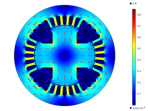
The simulations were made as a function of time and the materials were soft iron for the rotor core and the stator, air for the air gap and copper for the windings. From the simulation under normal operating conditions, Figure 5 was obtained, showing the magnetic flux density on the surface of the SM, the magnetic flux density is measured in Tesla [T].
|
| Figure 5. Magnetic flow density of SM in normal conditions |
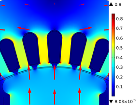
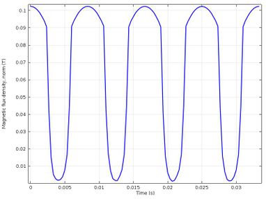
In Figure 5, it can be seen that the magnetic flux density has rotational symmetry that is maintained throughout the operation time. In addition, it is also observed how the magnetic paths are established, they leave a north pole and go to a south pole, in this way, they pass through the teeth and the stator crown. When the magnetic flux density passes through the teeth of the stator it becomes more concentrated due to the reduction in the available area since the normal pitch of the magnetic flux density is restricted, as shown in Figure 6. The highest density of magnetic flux within the SM is concentrated in the corners that join the rotor poles, and in this case, it has a value of and the minimum value of the magnetic flux density is around . In the stator teeth, the flow density reaches a maximum value of when in front of them are one of the poles of the rotor and a minimum value of when in front of them passes the space between two poles. In Table 3, we can find other values of the magnetic flux density on the surface of the SM, where it is shown that the magnetic flux density is constant in each of the poles and in Figure 7 it shows the behavior of the magnetic flux in the air gap.
|
| Figure 6. Magnetic flow density concentration in the stator teeth |
| Pole 1 | Pole 2 | Pole 3 | Pole 4 | |
|---|---|---|---|---|
| Flow in the center of the pole [T] | 0.26 | 0.26 | 0.26 | 0.26 |
| Flow on the right side of the pole [T] | 0.34 | 0.34 | 0.34 | 0.34 |
| Flow on the left side of the pole [T] | 0.34 | 0.34 | 0.34 | 0.34 |
| Flow at the midpoint of the crown [T] | 0.16 | 0.16 | 0.16 | 0.16 |
|
| Figure 7. Flow density in the air gap |
Figure 7 shows the variation in flow density as a function of time in the air gap during the operating time of the SM. This measurement was performed simulating the installation of a sensor to measure the magnetic flux in this region. Each one of the crests represents the density of magnetic flux in one pole and the valleys represent the density of flux in the space between them. In the previous graph we can also see how the magnetic flux decreases critically in the space between the poles.
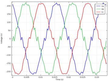
After conducting the magnetic flux density analysis, the induced voltages in the statistine coils were analyzed, their behavior is shown in Figure 8, where it can be seen that the voltages of the statistine coils show an approximately sinusoidal behavior with 120 ° lag, it has an effective value of 220 [V]. Likewise, it is also observed that the signal has harmonic components, this is due to the type of winding used in the study: composed of only one coil in each group of coils, six coils per phase and in a single layer.
|
| Figure 8. Statistical stresses of SM in normal conditions |
4.2 Short circuit analysis on a pole coil and no load connected
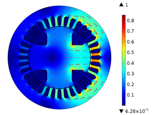
When a short circuit occurs in a coil, the number of turns is reduced. According to the law of Ampere applied to a coil of N tight turns, the magnetic flux will be reduced, since these variables are directly proportional. The excitation current is also directly proportional to the magnetic flux [12], therefore, to model the short circuit in the defective winding, a current with a value of 5% of the nominal current used in simulations under normal operating conditions was assumed. Figure 9 shows the behavior of the magnetic flux density in several regions of the SM.
|
| Figure 9. SM magnetic flow density with short circuit in a pole |
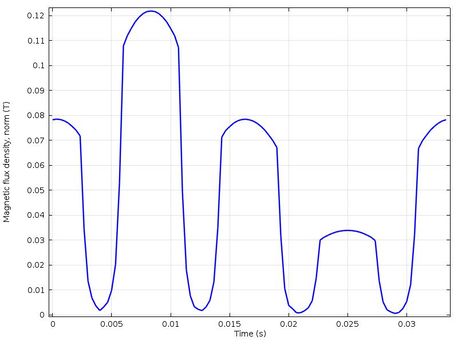
Figure 9 shows how the short circuit affects the magnetic flux density, decreasing the density value at the pole with short-coil and also at the adjacent poles, but it increases slightly at the pole opposite the short-circuit pole, as it is shown in Table 4 and Figure 10.
| Pole 1 | Pole 2 | Pole 3 | Pole 4 | |
|---|---|---|---|---|
| Flow in the center of the pole [T] | 0.32 | 0.20 | 0.08 | 0.20 |
| Flow on the right side of the pole [T] | 0.40 | 0.30 | 0.11 | 0.22 |
| Flow on the left side of the pole [T] | 0.40 | 0.22 | 0.11 | 0.30 |
| Flow at the midpoint of the crown [T] | 0.22 | 0.14 | 0.05 | 0.14 |
|
| Figure 10. Density of magnetic flow in the air gap |
Figure 10 shows that the crest with the lowest magnetic flux value represents the pole in short circuit and the crests that have intermediate value represent the poles that are next to the pole in short circuit, it can also be seen that the crest with higher value represents the pole that is on the opposite side of the pole in short circuit. In addition, the maximum value of the magnetic flux density has increased by 20%, but it must be remembered that this measurement of the magnetic flux density is taken in the air gap.
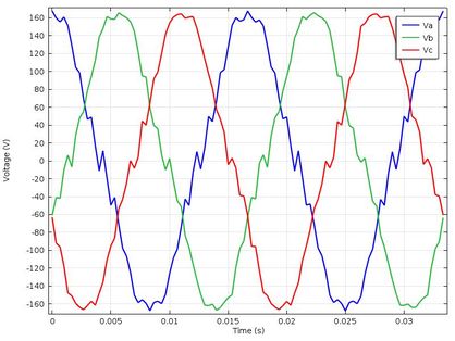
The short circuit in the winding of one of the poles will also affect the voltage in the stator winding, as it is shown in Figure 11.
|
| Figure 11. Statistical stresses of SM with pole in short circuit |
In Figure 10, it is shown how the amplitude of the stator voltage has decreased to a value close to 168.7 [V] due to the short circuit in the coil of one of the poles, but it can be seen that the signals have approximately sinusoidal behavior and the lag between them.
4.3 Analysis under normal operating conditions and with load connected
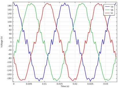
To analyze the operation of the SM with a load connected to the statistical winding a load of 7.2 KW was simulated, this is a resistive load connected in each of the phases of the statistical winding. The behavior of the magnetic flux density is the same as in Figure 5. Therefore, when connecting a load in each of the phases, the magnetic flux density will remain stable, and the magnetic flux density will have the same behavior and the same values as in Figure 7 , but the voltage amplitude of the statics windings will decrease as seen in the graph in Figure 12.
|
| Figure 12. Static strains of SM in normal state after connecting a load at the output |
The graph in Figure 12 shows how the output voltage decreases when a resistive load is connected to each of the phases. In this graph, it is observed that the value of the output voltage is approximately 195 [V], to normalize this value to 220 [V] you only have to increase the excitation current of the rotor coils, it will also increase the magnetic flux density inside the SM as shown in Figures 13 and 14, and in Table 5.
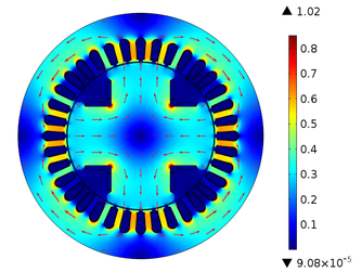
|
| Figure 13. Magnetic flow density of the SM in normal condition after normalizing the output voltage at 220 [V] |
| Pole 1 | Pole 2 | Pole 3 | Pole 4 | |
|---|---|---|---|---|
| Flow in the center of the pole [T] | 0.30 | 0.30 | 0.30 | 0.30 |
| Flow on the right side of the pole [T] | 0.39 | 0.39 | 0.39 | 0.39 |
| Flow on the left side of the pole [T] | 0.39 | 0.39 | 0.39 | 0.39 |
| Flow at the midpoint of the crown [T] | 0.19 | 0.19 | 0.19 | 0.19 |
In Figure 14 is shown that after increasing the value of the excitation current, the value of the magnetic flux density in the air gap and in the stator teeth also increased and the amplitude of the output voltage increased to 220 [V] showing the same behavior of Figure 8, showing that there is a direct proportionality relationship between the excitation current, the magnetic flux density and the voltage induced in the statics windings.
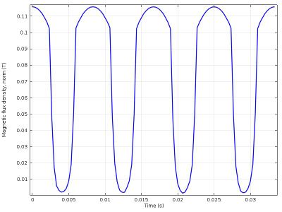
|
| Figure 14. Density of magnetic flow in the air gap |
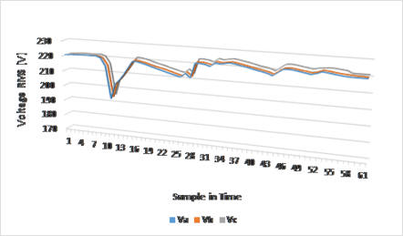
For the laboratory test, the synchronous machine rotor was moved through a primary machine mechanically attached to the shaft, as it is shown in Figure 15 . After starting the synchronous machine operation and stabilizing the output voltage at an rms value of 220 [V], the resistive load was connected, which caused a drop in the output voltage, for this reason the excitation current was increased to normalize the voltage again. Figure 16 shows this variation.
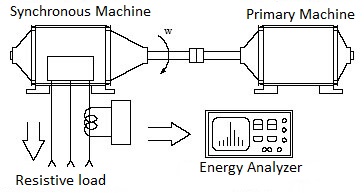
|
| Figure 15. Work bench [13] |
|
| Figure 16. SM statorial stresses measured in the laboratory test |
Figure 16 shows the behavior of stator voltages (peaks) in each of the phases before and after connecting the resistive load to each of these phases. It can be noted that the voltage in each phase corresponds to 220 [V] before connecting the load, from then in the voltage amplitude decreases to a value of approximately 194 [V], as happened in the simulations. After decreasing to this value, the voltage started to reestablish itself by varying the excitation current, after a certain time the voltage in each phase stabilizes at 220 [V].
4.4 Analysis in short-circuit and with connected load
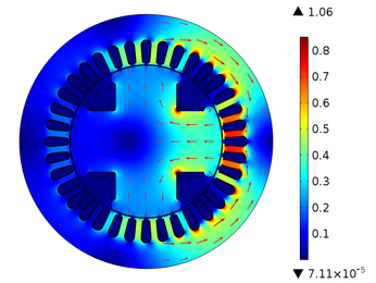
For this last analysis, the same resistive load of the previous simulations was simulated, a short circuit of 5% of the total value of the coil was chosen, this value practically leaves the pole coil with a total short circuit. Figure 17 shows the behavior of the magnetic flux density in the different regions of the SM when it has a connected load and has a short circuit in the coil of one of the poles.
|
| Figure 17. SM magnetic flow density with short circuit pole and load connected |
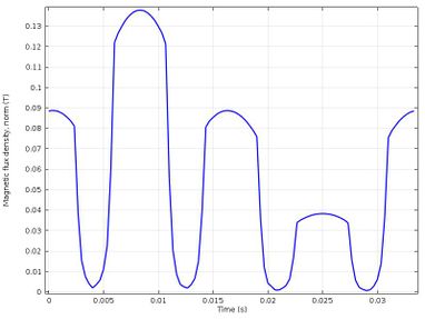
Figure 17 shows that the distribution of the magnetic flux density in the teeth of the stator and in the crown of the poles is not uniform due to the short circuit present in one of the poles, this behavior is described in Figure 18 and Table 6.
| Pole 1 | Pole 2 | Pole 3 | Pole 4 | |
|---|---|---|---|---|
| Flow in the center of the pole [T] | 0.36 | 0.23 | 0.09 | 0.23 |
| Flow on the right side of the pole [T] | 0.46 | 0.34 | 0.13 | 0.25 |
| Flow on the left side of the pole [T] | 0.46 | 0.25 | 0.13 | 0.34 |
| Flow at the midpoint of the crown [T] | 0.23 | 0.16 | 0.06 | 0.16 |
|
| Figure 18. Density of magnetic flow in the air gap |
In Figure 18 we can see how the magnetic flux density in the air gap behaves when one of the poles is short-circuited, it is observed that the maximum value of the magnetic flux density also increases, but this short-circuit will also affect the amplitude of the voltage in each of the phases as in the simulations in short-circuit without load, showing behavior and values similar to those of Figure 11.
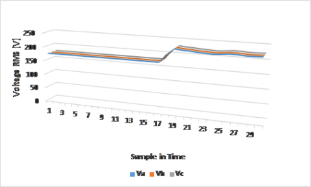
After increasing the excitation current to compensate for the output voltage, reduced by the short circuit, it is observed in Figure 19 that the results of the simulation are very close to the results obtained in the laboratory test.
|
| Figure 19. Density of magnetic flow in the air gap |
The test carried out in the laboratory consisted of making a short circuit in the coil of one of the poles of the real synchronous machine and representing 5% of its total value, after doing this, the operation of the synchronous machine started and a load was connected to the output. When the machine entered the steady state it was noticed that for the excitation current values of the SM working without short circuit and under load the output voltage decreased to 175 [V], It could be affirmed hat the short circuit affected the amplitude of the output voltage. Finally, the excitation current was increased to normalize the output voltage up to 220 [V]. Comparing the results of the SM simulation with the data shown in Figure 19, it can be inferred that the results of the simulation are close to the data of the laboratory test, when in the simulation a short circuit was made at a pole, the voltage value decreased until 165.8 [V] and in the laboratory test when this short circuit was made the voltage value decreased to approximately 175 [V], presenting an error of 5.2%. The graph in Figure 18 also shows that the voltage normalizes to 220 [V] after increasing the excitation current, as well in the simulations and laboratory tests with the machine operating with a short circuit.
5. Conclusions
As the analysis of the results of the simulations of the SM in different operating conditions can show that a magnetic flux density has radial symmetry and it is also uniform in some regions of the SM, the teeth and crowns of the poles, this happens when the machine works under normal conditions. When there is a short circuit in the coil of one of the poles, the density of magnetic flux will not be uniform in the different regions of the poles and the radial symmetry will be lost. In addition, the density of magnetic flux in the short-circuited pole will decrease, being proportional to the size of the short circuit. It also affects the flux density generated by the poles without short in addition to decreasing the amplitude of the output voltage in each of the phases, but does not change its waveforms.
The air gap is the ideal place to measure the magnetic flux generated by the poles and to detect short-circuit failures, since at these points the flow density behavior pattern can be perceived.
The results obtained from the simulations made in the finite element software allow for a more detailed analysis and to understand the behavior of the magnetic flux density in the different regions of the SM. This work can be very useful for research, especially for the development of magnetic flow sensors applied to synchronous generators because the data obtained with them can be compared with the results obtained in this research. The results of this project also allow us to understand the flow behavior in each of the materials that are part of the SM, as well as to determine a relationship between the magnetic flux density and the output voltage of the SM, including seeing how the composition of the SM ( number of slots) changes the behavior of the voltage signal.
Acknowledgements
This work was partially supported by Fundação de Amparo à Pesquisa do Estado de Minas Gerais (FAPEMIG).
References
[1] Chapman S. Máquinas eléctricas. McGraw Hill. 3rd ed., 2000.
[2] Fraile Mora J. Máquinas eléctricas. McGraw Hill, 5th ed, Madrid, Spain, 2003.
[3] Antunes H. Modelagem matematica do gerador sincrono trifásico de pólos salientes. Universidade Federal de Viçosa, Viçosa, Brazil, 2007.
[4] Meunier G. The finite element method for electromagnetic modeling. Wiley, ISTE, 1st ed., London, England, 2008.
[5] Bastos J., Sadowski N. Electromagnetic modeling by finite element methods. New York, United States, 2003.
[6] Gavela P., Morales J. Medición y simulación de campos electromagnéticos con elementos finitos de las subestaciones # 2, 3, 4, y 5 pertenecientes a la Empresa Electrica Centro Sur (EERCS). Universidad Politécnica Salesiana, Cuenca, Ecuador, 2008.
[7] Ratnajeevan S., Hoole H. Computer-aided analysis and design of electromagnetic devices. Elsevier, New York, United States, 1989.
[8] Geyverson P. Projeto de uma máquina síncrona com ímã permanente no rotor. Universidade de São Paulo, São Carlos, Brazil, 2011.
[9] Silwal B. Computation of eddy currents in a solid rotor induction machine with 2D and 3D FEM. AALTO University, Espoo, Finland, 2012.
[10] Albalat G. Diseño y simulación de una máquina eléctrica lineal de reluctancia conmutada con un programa informático. Universitat Rovira I Virgili, Tarragona, Spain, 2012.
[11] Baltierra A., Cervantes I., Escarela R. Simulación de un generador síncrono mediante el método de elemento finito con aplicación a control. Congreso Anual de la AMCA, Mexico D.F., 2004.
[12] Serway R. Electricidad y magnetismo. McGraw-Hill, 3rd Ed., 2000.
[13] Flores R., Asiaín T. Diagnóstico de fallas en máquinas eléctricas rotatorias utilizando la técnica de espectros de frecuencia de bandas laterales. Información Tecnológica, 22(4):73-84, 2011.
Document information
Published on 12/01/21
Accepted on 03/12/20
Submitted on 30/06/20
Volume 37, Issue 1, 2021
DOI: 10.23967/j.rimni.2020.12.002
Licence: CC BY-NC-SA license
Share this document
Keywords
claim authorship
Are you one of the authors of this document?