Virtual Laboratories as a Strategy for Teaching Improvement in Math Sciences and Engineering in Bolivia

Latest revision as of 12:01, 22 June 2020

Abstract

STEM education is a strategy based on four disciplines (science, technology, engineering and mathematics), integrated in an innovative interdisciplinary approach. Although, the concept of STEM education is more relevant today, the discussion of a teaching model with special attention in the four subjects aforementioned began in the early 2000s. Taking into account this context, the strategy presented in this paper has been disseminated in Bolivia's main universities for the last five years. A country that has not yet managed to associate basic disciplines such as calculus, matrix algebra, and/or differential equations to solve problems of an applicative nature, that is, to establish the link between theory and practice. To establish the connection, it is necessary to deduce differential equations associated with practical problems; solve these equations with numerical methods, appeal to the simulation concept to later introduce programming languages like Python/VPython to build virtual laboratories. The classical problem addressed for this purpose is the satellite of two degrees of freedom.

keywords

Numerical methods, Programming languages, Simulation, Satellite control.

1 INTRODUCTION

STEM education is a strategy that proposes teaching based on four disciplines (science, technology, engineering and mathematics), integrated in an innovative and interdisciplinary approach [1]. The United States, the most innovative country, home to the world's top startups, has identified the need to invest in these disciplines as a priority. For these reasons and looking for a high level of competitiveness in the professional market, several universities around the world have introduced computing tools (Matlab-Simulink®, Mathematica, Python, etc.), in their teaching programs which has helped to address a wide type of problems and increase the level of understanding not only in sciences and engineering but also in other STEM areas [2-4].

Some universities in Brazil, Chile, Argentina and Colombia have already adopted the STEM concept [5]. Contrary to this trend in South America, most universities in Bolivia do not apply it. There is a resistance to a methodological change, and to the use of technology to improve education, at the same time research works are just beginning. In this sense, this document aims to present the strategy proposed in Bolivia to improve education through the implementation of virtual laboratories. The strategy presented has been disseminated in the main Bolivian universities (Bolivia has 10 state and over 30 private universities).

1.1 Bolivian problem

For the past five years, different activities have been executed with several Bolivian universities (advanced courses, symposia and recently, master's degrees courses) [6].

As a result of this interaction, it has become clear that some universities face several problems, among them, the lack of funds for the purchase of specialized software. At the same time they have been slow in updating their study programs and in the application of modern techniques in higher education. These and other aspects do not allow universities to be much more innovative. These problems increase due to structural failures in high school education (i.e. reduced hours in math sciences) and successive changes of methodology in teaching schools where teachers of basic school are trained [7].

The strategy presented in this document was disseminated in several Bolivian universities as a proposal to improve teaching in math sciences and engineering. In the proposal, was also considered students' comments such as, what do I do with so much mathematics?, Calculus I, II, III , differential equations, numerical methods?, where do I apply all this?. These questions are constantly being asked because math science disciplines are still administered without a link of applicative character. This work tries to establish this link as the main contribution to Bolivian universities [7].

1.2 The proposal strategy

Figure 1: Chronological sequence strategy

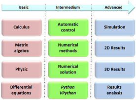
Figure 1 illustrates the chronological sequence of the strategy that starts from the basic cycle that contains disciplines such as calculus and physics, an intermediate cycle that provides knowledge in numerical methods, automatic control and software languages such as Python/VPhyton. In sequence there are advanced concepts such as simulation and visualization and analysis of the obtained results.

In this sense, section 2 presents basic modeling concepts, section 3 presents a summary of the Python and Vpython tools for building graphical interfaces. Section 4 presents the problem of the two degrees of freedom satellite, its mathematical modeling, simulation and graphical interface. Section 5 contains the corresponding control problem. Finally, some conclusions and discussions are presented in section 6.

2 BASIC CONCEPTS

Most of the phenomena that occur in nature involve the variation of one quantity related other, leading naturally to mathematical models based on differential equations ¹ [8]. To obtain these equations, physical laws such as: Newton's second law, the law of conservation of energy, Kirchhoff's law, or those corresponding to a particular phenomenon are used. Some of these basic concepts are presented below.

(¹) They can also be algebraic equations.

2.1 Euler-Lagrange equations

A dynamic system with ${\textstyle n}$ degrees of freedom in generalized coordinates ¹ ${\textstyle q\in {\mathcal {R}}^{n}}$ and external forces ${\textstyle Q_{\ell }\in {\mathcal {R}}^{n}}$ , is described by the following Euler-Lagrange equation:

(1)

where:

(2)

corresponds to Lagrange function, ${\textstyle {\mathcal {T}}({\dot {q}},q)}$ is the kinetic energy and ${\textstyle {\mathcal {V}}(q)}$ , is potential energy.

The external forces considered are: friction, control input and the interaction between system and environment. The control vector considered is ${\textstyle u\in {\mathcal {R}}^{m}}$ . Friction forces are represented as ${\textstyle {\dfrac {\partial {\mathcal {F}}}{\partial {\dot {q}}}}({\dot {q}})}$ , where ${\textstyle {\mathcal {F}}({\dot {q}})}$ is the function of Rayleigh. In summary, the following external forces are considered:

(3)

where ${\textstyle Q_{\epsilon }}$ is the signal that contains external perturbations.

(¹) Let the set of variables $q_{1}$ , $q_{2}$ , $q_{3}$ and $q_{4}$ .

2.2 Mathematical representation

Models are represented by the following differential equations:

(4)

where ${\textstyle {\dot {x}}_{i}}$ denotes the derivative of ${\textstyle x_{i}}$ related at the time ${\textstyle t}$ while, ${\textstyle u_{1}}$ , ${\textstyle u_{2}}$ , ${\textstyle \dots ,u_{m}}$ , are the control variables and ${\textstyle x_{1},x_{2},\dots ,x_{n}}$ , correspond to the state variables, with ${\textstyle x\in {\mathcal {R}}^{n}}$ and ${\textstyle u\in {\mathcal {R}}^{m}}$ . The output variables are given by:

(5)

where ${\textstyle y\in {\mathcal {R}}^{p}}$ . Finally, equations (4) and (5) can be written as:

${\dot {x}}=f(t,x,u)$	(6)
$y=g(t,x,u)$	(7)

2.3 Equilibrium points

The equilibrium points are solutions of the equations (6) and (7) such as:

2.3.1 Definition

The point $x=x^{*}$ in the state space is a equilibrium point of ${\dot {x}}=f(t,x)$ if:

(8)

in another form, the equilibrium point is $(x^{*},u^{*})$ .

In simple problems (like the pendulum), the solution of equation (8) is straightforward [9]. However, when the degree of difficulty increases, extracting operating conditions is also more complex; an aircraft is a good example [10,11].

2.4 Linearization

The linearization at a point of operation is a common practice in engineering to analyze nonlinear systems. Once the linear model is obtained, its analysis is done with widely used tools [12]. However, the approximation around an operation point offers the local behavior of the non-linear system and not the global behavior in which we are interested. One of the most common methods to perform the linearization is the expansion by series of Taylor, effective for small variations around the operation point [13,14].

3 PYTHON AND VPYTHON LANGUAGES

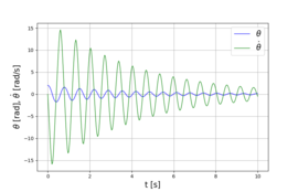
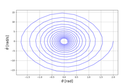
Python is a high-level interpreted language with sequential commands developed at the end of the 1980s by Guido van Rossum at the National Research Institute of Mathematics and Computer Science in the Netherlands [15]. This language is widely used in large organizations due to its multiple programming paradigms. It provides standard libraries that include areas such as: chain operations, internet, web service tools, operational system interfaces and protocols. The Python interpreter is developed under an open source license, which makes it free to use and distribute, even for commercial purposes [16]. This last characteristic makes it ideal for its use, since it dispenses the license payment reducing costs in universities and industries. Figure 2 presents a Python code example (corresponds to the simples pendulum problem [17]). Figs. 3a and 3b allow to verify the behavior of a simples pendulum in two dimensions.

from numpy import *
import numpy as np from scipy.integrate
import odeint import matplotlib.pyplot as plt
# Parameters
g = 9.8; L = 0.1; m = 0.2; u = 0.0; k = 0.1

def eqs_mov(state, t, p): # dy/dt = f(t,y)
y1, y2 = state
dydt = np.zeros_like(state)
dydt = [y2,
-(g/L)*np.sin(y1)-(k/m)*y2 + u/(m*L**2)]
return dydt
# Initial Conditions
p = [g, L, k, u, m]; state = [2., 0]
t =np.linspace(0,10,300); print (t)
sol = odeint(eqs_mov,state,t,args=(p,))

Figure 2: Python code for pendulum model

(a) Angular position and rate

(b) Phase diagram

Figure 3: Simples pendulum behavior

In sequence to the development of the language Python in the spring and summer of the year 2000, with the help of David Andersen, Ruth Chabay, Ari Heitner, Ian Peters and Bruce Sherwood, David Scherer creates Visual, a module for Python that was not only relatively simple to use, but also allowed the development of objects in three dimensions. The combination of Python and Visual is called VPython which allows users to create objects such as spheres, cylinders and 3D cones and displays them in a window, which facilitates the creation of three-dimensional visualizations. This last feature has made VPython an essential tool for the creation of virtual laboratories [18].

Figure 4: Virtual environment for double pendulum

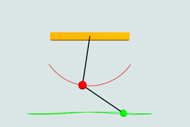
The three-dimensional representation of the double pendulum is illustrated in Figure 4.

4 TWO DEGREE OF FREEDOM SATELLITE PROBLEM

The orbit of the satellite of two degrees of freedom with mass

is illustrated in Figure 5, can be described by two non-linear and coupled equations obtained from the sum of the kinetic energy due to the tangential component

and radial component of velocity

. It is assumed that the satellite has traction in these directions, thus the magnitude of the forces are

and

respectively.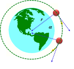

Figure 5: Two degree of freedom satellite

This problem is well known in the area of automatic control, but, is not studied in the Bolivia education program. Also, its importance lies in that it is a problem with multiple inputs and multiple outputs (MIMO) [19,20].

4.1 Mathematical model

The total kinetic energy of the satellite of Figure 5 is given by:

(9)

The equations (9) and (2) allow obtaining the mathematical model of this problem [wolovich94].

4.2 Computational solution

Figure 6a illustrates the results obtained for

and

. It is verified that

moves away from its initial condition through a ramp, for this reason the derivative

tends to be a constant.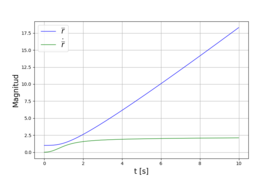

(a) Radial position and rate

(b) Angular position and rate

Figure 6: Two degree of freedom satélite in two dimensions

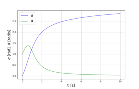
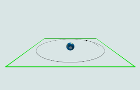
Figure 6b illustrates the results obtained for ${\textstyle \alpha (t)}$ and ${\textstyle {\dot {\alpha }}(t)}$ . It is verified that ${\textstyle \alpha (t)}$ remains with constant behavior over time, for this reason the derivative ${\textstyle {\dot {\alpha }}(t)}$ tends to zero. In practice, it is expected that the satellite will describe a trajectory with angular velocity ${\textstyle {\dot {\alpha }}(t)}$ constant and with position ${\textstyle r(t)}$ constant also.

Figure 7 illustrates the tridimensional virtual environment for the satellite of two degrees of freedom.

Figure 7: Virtual environment for two degree of freedom satellite

5 AUTOMATIC CONTROL PROBLEM

The analysis and synthesis are performed by applying theory of optimal control and the technique of Linear Quadratic Regulator (LQR), method based on the linearization of dynamic systems, represented in the time domain [10, 12]. The control structure is presented in Figure 8.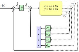

Figure 8: Generic control structure

5.1 Algorithm

The algorithm to find a control law ${\textstyle u}$ ¹ is given by:

$u=-[G_{x1}~G_{x2}~G_{x3}~G_{x4}]x+G_{i}\xi$	(10)
${\dot {\xi }}=r-y$	(11)

So that the feedback control law minimizes the performance index given by:

(12)

subject to the following state equation:

(13)

The gain matrix ${\textstyle G=[G_{x1}~G_{x2}~G_{x3}~G_{x4}~G_{i}]}$ is obtained from the solution of Riccati's equation.

(14)

where

and

are the augmented matrices. The optimal gain

can be obtained quickly using the Python Control toolbox. The code example used to calculate the gains is presented in Figure 9.

from control import* from slycot import*
from control.matlab import* import numpy as np

#Dates
Jm = 1.2; Bm = 0.1; Jl = 0.3; Bl = 0.05; m = 1; Kr = 0.5;

l= 0.5; g = 9.8;

A = [[0, 1],[-(g*l*m)/(Jl+Jm*Kr**2),
-(Bl+Bm*Kr**2)/(Jl+Jm*Kr**2)]];

B = [[0],[1/(Jm+(Jl/Kr**2))]];

C = [[1, 0],[0,1]]; D = [[0],[0]];

Aaum = [[A],[[0],[0]],[B],[1]] Baum = [[B],[0]]

Q = [[20, 0, 0],[0, 20, 0],[0, 0, 20]] R = 0.01

G, S, E =lqr(Aaum,Baum, Q, R)

Figure 9: Gains calculation Python code

(¹) In practice, the control variable $u$ , it is always limited to its maximum and minimum values.

5.2 Two degree of freedom satellite control

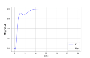
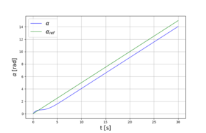
The controlled variables correspond to the position in relation to the center of the earth and the angular position of the satellite. The desired references are the unit for ${\textstyle |r|}$ and a ramp ${\textstyle 0.5t}$ for ${\textstyle \alpha }$ . Initials conditions of the integrator are ${\textstyle [0.8~0~0~1]^{T}}$ . The gain matrix ${\textstyle G}$ ( ${\textstyle r,{\dot {r}},\alpha ,{\dot {\alpha }}}$ ) obtained is:

(15)

Figure 10a shown the result of radial component

, where is verified that after of transient, the reference is reached.

(a) Radial distance

(b) Angular position

Figure 10: Closed loop results satellite TDOF

Figure 10b illustrates the result obtained for the angular position ${\textstyle \alpha (t)}$ , which follows the specified ramp with an offset, offset is characteristic of LQR control for ramp reference. To solve this problem it is necessary to study other control strategies [21].

6 CONCLUSIONS AND DISCUSSIONS

The main contribution of this proposal is applicative, simple examples show the link between theory and practice, the results obtained through simulations are evaluated in two and three dimensions, which allow the extensive use of virtual laboratories. The presented strategy is used in countries with high development indices, unfortunately this does not happen in Bolivia.

The summary of the methodology that addresses the problems presented is illustrated in Figure 11.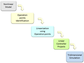

Figure 11: Summary of methodology

The main advantage of the presented strategy is for the country, which will benefit from a future generation with more professionals capable of working in the new industrial era. In this sense, it should be emphasized that this strategy will help in the training and motivation of the new Bolivian scientists in the short and long term period. This strategy is also attractive because programming languages like Python/Vpython are free. Let us not forget that these Virtual Laboratories can be quickly implemented on any computer and managed from a dedicated server that doesn't need the purchase of additional hardware.

6.1 Discussions

The total number of attendees where the strategy was presented reached approximately 500 among professors and students. During the presentations, a questionnaire was prepared asking what methodology was practiced by the participating universities. Figure 12 illustrates 12 presentations with an average of 40 participants by session. The total number of participants and the percentages that correspond to the methodologies Non-applied method and Applied method.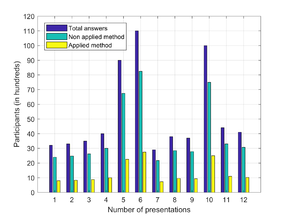

Figure 12: Number of presentations and answers of attendees

The result shows that 75% still administer subjects such as calculus, algebra and others isolated from practical applications. In this sense, the participating students evidenced the improvement in learning disciplines in science and engineering, integrated to the concepts of: modeling, programming languages, numerical methods and simulation. Following, some feedback from participating students are registered:

Great depth in the methodology, as rarely explained in our universities,
I did not see this method before, the learning is transparent and real world examples can be observed,
The strategy clearly shows the complete cycle that involves the deduction of mathematical models until the visualization of results in two and three dimensions.

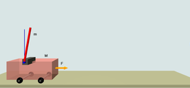
Furthermore, an interactive link is being developed where students can access to the presented problems and others [22]. Additionally, Figures 13a and 13b show the virtual environment for inverted pendulum and coupled springs problems.

(a) Inverted pendulum

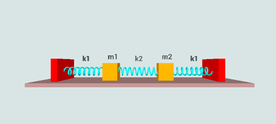
(b) Coupled springs

Figure 13: Additional virtual environments

The participating universities were suggested to use the strategy extensively, as well as to change their science and engineering study plans. After these recommendations where made, some universities have very slowly begun to make the suggested changes. Finally, during the dissemination of the strategy, two books were published, one in Bolivia and another in Brazil [17,20].

ACKNOWLEDGMENT

Thanks you to the participating universities, teachers and students who made possible this publication. Also, thank you to Juan Poma Rosas for English corrections and to SIB and CIEE of Cochabamba Bolivia for the financial support.

REFERENCES

[1] D. Deming and K. Noray, “STEM Careers and Technological Change”, Harvard University, 2018.

[2] J. Cortes Lopez and L. Jordar Sanches, “Introducción al Mathematica 7”, Universidad Politecnica de Valencia, 2011.

[3] A. Gilat, Matlab com Aplicações em Engenharia. Bookman, 2006.

[4] D. I. Wilson, “ Advanced Control Using Matlab”, Auckland University of Technology, 2015.

[5] L. M. Espinal and F. Silveira Segui, “ La generación de prácticas, proyectos o programas en educación STEM en el marco de una diplomatura virtual para América Latina”, Universidad de Alcalá Servicio de Publicaciones, 2019.

[6] F. J. Triveño Vargas, https://www.paginasiete.bo/gente/2016/10/27/equipo-bolivianos-desarrolla-algoritmos-para-controlar-drones-114891.html, Accessed: 2018-12-12, 2016.

[7] F. J. Triveño Vargas, http://www.lostiempos.com/oh/actualidad/20180312/universidad-no-quieren-dar-paso-adelante, Accessed: 2018-11-11, 2018.

[8] R. Kupferman, “Lecture Notes in Classical Mechanics ”, The Hebrew University, 2008.

[9] H.K. Khalil, “ Nonlinear Systems”, Prentice Hall Inc. Third Edition, 2002.

[10] B. Stevens and F. Lewis, “Aircraft Control and Simulation, 2nd Edition”, John Wiley Inc, 2003.

[11] F. J. Triveno Vargas and F. J. Oliveira Moreira and Pedro Paglione, “Longitudinal stability and control augmentation with robustness and handling qualities requirements using the two degree of freedom controller ”, Journal of the Brazilian Society of Mechanical Sciences and Engineering pp. 1843-1853, 2016.

[12] K. Ogata, “Engenharia de Controle Moderno”, Pearson Educaton, 5th Edition, 2011.

[13] E. L. Duke and R. F. Antoniewicz and Keith D. Krambeer, “ Derivation and Definition of a Linear Aircraft Model ”, NASA Reference Publication 1207, 1988.

[14] D. Gangsaas, J. Hodgkinson and C. Harden, “ Multidisciplinary Control Law Design and Flight Test Demonstration on a Business Jet ”, AIAA Guidance, Navigation and Control Conference and Exhibit pp. 1-25, 2008.

[15] J. Kusalaas ,“ Numerical Methods in Engineering with Python 3”, Cambridge University Press, 2013.

[16] M.L. Hetland , “ Beginning Python: From Novice to Professional, Second Edition”,Springer-Verlag New York, 2008.

[17] F. J. Triveño Vargas and Pedro Paglione, “ Aplicações de Modelagem, Simulação e Controle Com Ferramentas de Algebra Computacional ”, Editorial LTC, 2015.

[18] J. E. Villate, “Simulações com VPython”, https://def.fe.up.pt/python/vpython.html, Accessed: 2018-15-11, 2018.

[19] D. Siqueira, F. J. Oliveira Moreira and Pedro Paglione, “Robust Flight Control Design Supported by Flying Qualities Analysis”, AIAA Guidance, Navigation and Control Conference, South Carolina, pp. 415-428, 2007.

[20] F. J. Triveño Vargas and E. O. Pozo Irusta, “ Modelado, Simulación y Control de Sistemas Mecatronicos y Aeroespaciales con Matlab-Simulink® y Mathematica ${\textstyle ^{TM}}$ ”, Editorial Serrano, 2014.

[21] W. A. Wolovich,“Automatic Control Systems: Basic Analysis and Design”, Oxford University Press, 1994.

[22] H. Siles Alvarado, “Simulaciones en Ciencias y Tecnologia”, http://www.simcyt.org, Accessed: 2019-09-14, 2019.

@@ Line 204: / Line 204: @@
 sol = odeint(eqs_mov,state,t,args=(p,))
 </pre>
 |- style="text-align: center; font-size: 75%;"
@@ Line 246: / Line 245: @@
 The orbit of the satellite of two degrees of freedom with mass <math display="inline">M</math> is illustrated in Figure [[#img-5|5]], can be described by two non-linear and coupled equations obtained from the sum of the kinetic energy due to the tangential component <math display="inline">v_{t} = r(t) \dot{\alpha } (t) </math> and radial component of velocity <math display="inline"> v_{r} = \dot{r}(t)</math>. It is assumed that the satellite has traction in these directions, thus the magnitude of the forces are <math display="inline">F_{t}(t)</math> and <math display="inline">F_{r}(t)</math> respectively. <div id='img-5'></div>
-{| class="floating_imageSCP" style="text-align: center; margin: 1em auto; width: 100%;max-width: 100%;"
+{| class="floating_imageSCP" style="text-align: center; margin: 1em auto; width: 110%;max-width: 110%;"
 |-
 |[[Image:Review_159642103826-labVirtSpain_20.png|150px|Two degree of freedom satellite]]
@@ Line 311: / Line 310: @@
 ==5 AUTOMATIC CONTROL PROBLEM==
-The analysis and synthesis are performed by applying theory of optimal control and the technique of Linear Quadratic Regulator (LQR), method based on the linearization of dynamic systems, represented in the time domain [10, 12]. The control structure is presented in Figure [[#img-8|8]] . <div id='img-8'></div>
+The analysis and synthesis are performed by applying theory of optimal control and the technique of Linear Quadratic Regulator (LQR), method based on the linearization of dynamic systems, represented in the time domain [10, 12]. The control structure is presented in Figure [[#img-8|8]]. <div id='img-8'></div>
 {| class="floating_imageSCP" style="text-align: center; margin: 1em auto; width: 100%;max-width: 100%;"
 |-
@@ Line 508: / Line 507: @@
 ==ACKNOWLEDGMENT==
-Thanks you to the participating universities, teachers and students who made possible this publication. Also, thank you to Juan Poma Rosas for English corrections and to SIB and CIEE of Cochabamba Bolivia for the financial support
+Thanks you to the participating universities, teachers and students who made possible this publication. Also, thank you to Juan Poma Rosas for English corrections and to SIB and CIEE of Cochabamba Bolivia for the financial support.
 ==REFERENCES==
-[1] D. Deming and K. Noray, “ STEM Careers and Technological Change”, Harvard University, 2018.
+[1] D. Deming and K. Noray, “STEM Careers and Technological Change”, Harvard University, 2018.
 [2] J. Cortes Lopez and L. Jordar Sanches, “Introducción al Mathematica 7”, Universidad Politecnica de Valencia, 2011.
@@ Line 522: / Line 521: @@
 [5] L. M. Espinal and F. Silveira Segui, “ La generación de prácticas, proyectos o programas en educación STEM en el marco de una diplomatura virtual para América Latina”, Universidad de Alcalá Servicio de Publicaciones, 2019.
-[6] F. J. Triveño Vargas, http://www.paginasiete.bo/gente/2016/10/27/equipo-bolivianos-desarrolla-algoritmos-para-controlar-drones-114891.html, Accessed: 2018-12-12, 2016.
+[6] F. J. Triveño Vargas, https://www.paginasiete.bo/gente/2016/10/27/equipo-bolivianos-desarrolla-algoritmos-para-controlar-drones-114891.html, Accessed: 2018-12-12, 2016.
-[7] F. J. Triveño Vargas, “UNIVERSIDAD: No quieren dar un paso adelante”, http://www.lostiempos.com/oh/actualidad/20180312/universidad-no-quieren-dar-paso-adelante), Accessed: 2018-11-11, 2018.
+[7] F. J. Triveño Vargas,  http://www.lostiempos.com/oh/actualidad/20180312/universidad-no-quieren-dar-paso-adelante, Accessed: 2018-11-11, 2018.
 [8] R. Kupferman, “Lecture Notes in Classical Mechanics ”, The Hebrew University, 2008.
@@ Line 536: / Line 535: @@
 [12] K. Ogata, “Engenharia de Controle Moderno”, Pearson Educaton, 5th Edition, 2011.
-[13]  E. L. Duke and R. F. Antoniewicz and Keith D. Krambeer,  “Derivation and Definition of a Linear Aircraft Model ”,  NASA Reference Publication 1207, 1988.
+[13]  E. L. Duke and R. F. Antoniewicz and Keith D. Krambeer,  “ Derivation and Definition of a Linear Aircraft Model ”,  NASA Reference Publication 1207, 1988.
-[14] D. Gangsaas, J. Hodgkinson and C. Harden, “ Multidisciplinary Control Law Design and Flight Test Demonstration on a  Business Jet”, AIAA Guidance, Navigation and Control Conference and Exhibit pp. 1-25, 2008.
+[14] D. Gangsaas, J. Hodgkinson and C. Harden, “ Multidisciplinary Control Law Design and Flight Test Demonstration on a  Business Jet ”, AIAA Guidance, Navigation and Control Conference and Exhibit pp. 1-25, 2008.
 [15] J. Kusalaas ,“ Numerical Methods in Engineering with Python 3”, Cambridge University Press, 2013.
@@ Line 546: / Line 545: @@
 [17] F. J. Triveño Vargas and Pedro Paglione, “ Aplicações de Modelagem, Simulação e Controle Com Ferramentas de Algebra Computacional ”, Editorial LTC, 2015.
-[18] J. E. Villate, “Simulações com VPython”, https://def.fe.up.pt/python/vpython.html,Accessed: 2018-15-11, 2018.
+[18] J. E. Villate, “Simulações com VPython”, https://def.fe.up.pt/python/vpython.html, Accessed: 2018-15-11, 2018.
 [19] D. Siqueira, F. J. Oliveira Moreira and Pedro Paglione, “Robust Flight Control Design Supported by Flying Qualities Analysis”, AIAA Guidance, Navigation and Control Conference, South Carolina, pp. 415-428, 2007. <div id="cite-19"></div>
-[20] F. J. Triveño Vargas and E. O. Pozo Irusta, `` Modelado, Simulación y Control de Sistemas Mecatronicos y Aeroespacialescon Matlab®y Mathematica<math display="inline">^{TM}</math> '', Editorial Serrano, 2014.
+[20] F. J. Triveño Vargas and E. O. Pozo Irusta, “ Modelado, Simulación y Control de Sistemas Mecatronicos y Aeroespaciales con Matlab-Simulink® y Mathematica<math display="inline">^{TM}</math> ”, Editorial Serrano, 2014.
-[21] W. A. Wolovich,“Automatic Control Systems: Basic Analysis and Design ”, Oxford University Press, 1994.
+[21] W. A. Wolovich,“Automatic Control Systems: Basic Analysis and Design”, Oxford University Press, 1994.
-[22] H. Siles Alvarado, “ Simulaciones en Ciencias y Tecnologia ”, http://www.simcyt.org, Accessed: 2019-09-14, 2019.
+[22] H. Siles Alvarado, “Simulaciones en Ciencias y Tecnologia”, http://www.simcyt.org, Accessed: 2019-09-14, 2019.