Revision as of 00:30, 23 February 2020 (view source) Htabares (talk | contribs) (Created page with "<!-- metadata commented in wiki content ==A method to calculate the numerical integration and degree of fluctuation of fractally spaced data.== '''Héctor Tabares-Ospina<su...")	Revision as of 00:34, 23 February 2020 (view source) Htabares (talk | contribs) m (Htabares moved page Draft Tabares-Ospina 730588725 to Tabares-Ospina Osorio 2020a) Newer edit →
(No difference)

---

Revision as of 00:34, 23 February 2020

Abstract: This article proposes a new numerical method to calculate the integral of a function, using the trapezoid rule, but spacing the intervals fractally, with the purpose of discovering other complementary observations in relation to the degree of fluctuation of the function studied, a parameter that can be included in conventional numerical integration methods. The results are compared with the conventional method of generalized Trapezoid Rule, in which the intervals are equally spaced.

This is then a new contribution that extends universal knowledge on the subject.

AMS subject classifications: 65D30, 65Yxx, 65M12.

Key words : Numerical Integration; Computer aspects of numerical algorithms, Fractal dimension.

1. Introduction

A semi-geometric element is “fractal” when it contains a repetitive structure in different scales with self-similarity characteristics. The fractal concept was developed by the mathematician Benoit Mandelbrot in the 1970s [1]. In fact, nature provides examples of fractals such as snowflakes, ferns, peacock feathers, and romanesco broccoli. Fractal theory has been used to analyze data and obtain relevant information in highly complex problems such as biology [2,3], health sciences [4–8], securities markets [9], network communications [10–12], and others. Other interesting applications are related with the electrical power. In [13], authors presented a new methodology to analyze the dynamics of the daily power demand by using the curve formed by attractors that move in the complex plane over the Mandelbrot set according to the law dictated by the load curve.

The fractal dimension is concept that indicate the degree of fluctuation of any function. In [14] authors explored fractal analysis in order to discriminate between pathological and healthy retinal texture.

Other example is [15], where bentonite is studied when it is affected by a corrosion process in alkaline solution. The fractal dimensions of bentonite specimens at different stages of the corrosion process were obtained from ${\textstyle {N}_{2}}$ adsorption and swelling deformation tests, and the results of both methods suggested that the fractal dimension tends to increase with duration of the corrosion process.

[16] used fractal dimension to describe the behavior of auriferous veins across the boreholes.

[17] used fractal dimension as an indicator of compactness. The fractal dimension of demolition waste was calculated by fitting the particle size demolition curves into the fractal model.

The exhaust stream of internal combustion engines contains soot agglomerates with fractal geometries. In [18] the fractal dimension of an agglomerate is estimated from the combination of its volume and a characteristic radius.

In [19] the fractal dimensions of aggregates and cement are discussed. A comprehensive understanding of the fractal properties of concrete meso-structure is important because it is associated with the complex and random mechanical behaviors of the concrete.

In [20], authors present a novel method to estimate pedestrian flow in uncontrolled environments by using the fractal dimension measured through the box-counting algorithm, which does not neither require the use of image pre-processing and nor intelligent algorithms.

In [21] fractal dimension is applied to study the growth of urban people of Beijing city, in China.

Finally, [22] present the spatial morphology of the soft agglomerate, such as maltodextrin, quantified by fractal dimension.

The previous Articles are the basis for the new contribution, considering the following hypothesis: The degree of fluctuation of a function is calculated using fractal dimension method. The fractal segments obtained also may be used to calculate the area under the curve, integrating the function using standard trapezoid rule, with fractally spaced data.

The most outstanding reference is [23], where a method to do numerical integration is studied when the original ‘‘signal’’ shows experimentally some kind of self-similarity.

Finally, this document is organized as follows. Section 2 provides a brief explanation of fractal dimension and the methods to do the numerical integration using trapezoid rule. Section 3 presents the method applied in this research and the algorithm used. Section 4 reports and discusses the most relevant results. Finally, the main conclusions of this research work are summarized in Sec. 5

The concept of fractal dimension is introduced with respect to the fact that most objects of nature do not have an entire dimension, but they are in a fractional dimension and this dimension must be greater than its topological dimension. The fractal dimension is a dimensionless numerical measure that indicates how the length, area, or volume varies, depending on the size of the measurement element used. It is calculated with various box sizes, making a linear fit to a ${\textstyle Log(N\left(r\right))}$ graph over ${\textstyle Log(r)}$. As the size of the boxes reduces their area, the points in the logarithmic graph align more and more and the fractal dimension can be calculated as the slope of the line that joins them, by the expression:

${\displaystyle D=Log(N\left(r\right))/Log(r)}$

(1)

Where ${\textstyle r}$ is the size of the measure element used, and ${\textstyle N\left(r\right)}$ is the length, area or volume related.

In conclusion, D allows to determine the complexity of the set space under study. [24]

A detailed study on the numerical methods of integration is beyond the scope of this unit. Full information is provided in (Mathews, J, Fink, K, 2000). A recount on the matter, are presented below:

It is sought to calculate the definite integral ${\textstyle \int _{a}^{b}f\left(x\right)dx}$, using the Newton-Cótes methods, which integrates an interpolation polynomial that approximates ${\textstyle f\left(x\right)}$ in ${\textstyle \left[a,b\right]}$ . Therefore, these are methods, according to the interpolation polynomial considered. In the case of linear and quadratic interpolations, these methods are called Trapeze Method and Simpson Method, respectively.

The Trapezoid Method is a Newton-Cotes Method based on linear interpolation. With the purpose of integrating ${\textstyle f\left(x\right)}$ from the point ${\textstyle \left(a,f\left(a\right)\right)}$ to ${\textstyle \left(b,f\left(b\right)\right)}$ , ${\textstyle f\left(x\right)}$ is approximated by its linear interpolation polynomial in ${\textstyle \left[a,b\right]}$

And so

${\displaystyle I=\int _{a}^{b}f\left(x\right)dx\approx \int _{a}^{b}{P}_{1}\left(x\right)dx={\frac {b-a}{2}}\left(f\left(a\right)+f(b)\right)}$

The value of the integral ${\textstyle I}$ approximates the area of the trapezoid determined by the lines ${\textstyle x=}$${\displaystyle a,\,x=b}$, the axis of abscissa and the line that joins the points ${\textstyle \left(a,f\left(a\right)\right)}$ and ${\textstyle \left(b,f\left(b\right)\right)}$ . Another important aspect is also the knowledge of the degree of precision of the numerical solution.

The expression of the linear interpolation error, assuming that ${\textstyle f\left(x\right)}$ is continuous and derivable twice in the interval ${\textstyle \left[a,b\right]}$ :

${\displaystyle f\left(x\right)={P}_{1}\left(x\right)+\,\epsilon \left(x\right)}$

We will have then

${\displaystyle I=\int _{a}^{b}f\left(x\right)dx={\frac {b-a}{2}}\left(f\left(a\right)+f(b)\right)+E}$

Where the error of numerical integration ${\textstyle E}$ is:

${\displaystyle E=\int _{a}^{b}\epsilon \left(x\right)dx={\frac {{f}^{''}(\delta )}{2}}\int _{a}^{b}\left(x-a\right)\left(x-b\right)dx}$

Integrating this last expression and naming ${\textstyle h=}$${\displaystyle b-a}$, it is concluded that:

${\displaystyle E=-{\frac {{h}^{3}}{12}}{f}^{''}\left(\delta \right)\Rightarrow \left|E\right|\leq \left|{\frac {{h}^{3}}{12}}{M}_{2}\right|}$

${\textstyle {M}_{2}}$is the maximum value reached by the second derivative of the function in the given interval ${\textstyle \left[a,b\right]}$ . The demonstration of this general result can be found in advanced texts on numerical integration.

If the interval in which the integral is carried out is large, the Simple Trapeze Method is usually very imprecise. To improve accuracy, it is possible to subdivide the interval into smaller ones and apply the Simple Method to each one.

Thus, the compound or generalized Trapeze Method consists in taking a partition ${\textstyle P=}$${\displaystyle \left\{{x}_{0},{x}_{1},\ldots ,{x}_{n}\right\}}$ from ${\textstyle \left[a,b\right]}$ , ${\textstyle \left({x}_{0}=\right.}$${\displaystyle \left.a,\,\,{x}_{n}=b\right)}$ , equiespaced, that is: ${\textstyle {x}_{i+1}-}$${\displaystyle {x}_{i}=h}$, ${\textstyle \forall i=}$${\displaystyle 1,\ldots ,n.}$ We will have so:

${\displaystyle h={\frac {b-a}{n}}}$

Taking into account the basic properties of the definite integral:

${\displaystyle \int _{a}^{b}f\left(x\right)dx=\int _{{x}_{0}}^{{x}_{1}}f\left(x\right)dx+\int _{{x}_{1}}^{{x}_{2}}f\left(x\right)dx+\ldots +}$${\displaystyle \int _{{x}_{n-1}}^{{x}_{n}}f\left(x\right)dx}$

And applying to each integral the simple method:

${\displaystyle \int _{a}^{b}f\left(x\right)dx\approx {\frac {h}{2}}\left(f\left({x}_{0}\right)+f\left({x}_{1}\right)\right)+{\frac {h}{2}}\left(f\left({x}_{1}\right)+f\left({x}_{2}\right)\right)+\ldots +{\frac {h}{2}}\left(f\left({x}_{n-1}\right)+f\left({x}_{n}\right)\right)}$

${\displaystyle ={\frac {h}{2}}\left(f\left({x}_{0}\right)+2\left(f\left({x}_{1}\right)+f\left({x}_{2}\right)+\ldots +\right.\right.}$${\displaystyle \left.\left.f\left({x}_{n-1}\right)\right)+f\left({x}_{n}\right)\right)}$

Therefore, we have the final expression for the Generalized Trapeze Method:

${\displaystyle \int _{a}^{b}f\left(x\right)dx\cong {\frac {h}{2}}\left(f\left(a\right)+2\sum _{i=1}^{n-1}f\left({x}_{i}\right)+f\left(b\right)\right)}$

With regard to the integration error, it will be equal to the sum of the errors of each of the applications of the simple method:

${\displaystyle E={E}_{1}+{E}_{2}+\ldots +{E}_{n}=-{\frac {{h}^{3}}{12}}{f}^{''}\left({\epsilon }_{1}\right)-}$${\displaystyle {\frac {{h}^{3}}{12}}{f}^{''}\left({\epsilon }_{2}\right)-\ldots -{\frac {{h}^{3}}{12}}{f}^{''}\left({\epsilon }_{n}\right)}$

If we call ${\textstyle {M}_{2}}$ the maximum of the function ${\textstyle {f}^{''}\left(x\right)}$ in ${\textstyle \left[a,b\right]}$ , we will have:

${\displaystyle \left|E\right|\leq \left|{\frac {{h}^{3}}{12}}n{M}_{2}\right|=\left|{\frac {\left(b-a\right)}{12}}{h}^{2}{M}_{2}\right|}$

(2)

This means that the error is of order ${\textstyle O\left({h}^{2}\right)}$ .

In [25] is indicated that all numerical integration formulas have been based on equally spaced data. However, in practice there are many situations in which this assumption is not met and there are segments of unequal sizes. For example, experimentally obtained data, or fractally spaced data, are often of this type. In such cases, one method is to apply the trapezoid rule to each segment and add the results, as indicated in equation (2), where ${\textstyle {h}_{i}=}$ the width of segment ${\textstyle i}$.

Assume that ${\textstyle y=}$${\displaystyle f\left(x\right)}$ be continuous, and possess continuous derivatives in ${\textstyle \left[{x}_{0},{x}_{n}\right].}$ Expanding ${\textstyle y=}$${\displaystyle f\left(x\right)}$ in Taylor polynomials [26] around ${\textstyle x=}$${\displaystyle {x}_{0}}$, the result obtained is

${\displaystyle y\left(x\right)={y}_{0}+{\frac {\left(x-{x}_{0}\right)}{1!}}{y}_{0}^{'}+{\frac {{\left(x-{x}_{0}\right)}^{2}}{2!}}{y}_{0}^{''}+}$${\displaystyle \ldots }$

(3)

Now, using (3)

${\displaystyle ={\left[{y}_{0}x+{\frac {{\left(x-{x}_{0}\right)}^{2}}{2}}{y}_{0}^{'}+{\frac {{\left(x-{x}_{0}\right)}^{3}}{6}}{y}_{0}^{''}+\ldots \right]}_{{x}_{0}}^{{x}_{1}}}$

${\displaystyle ={y}_{0}\left({x}_{1}-{x}_{0}\right)+{\frac {{\left({x}_{1}-{x}_{0}\right)}^{2}}{2}}{y}_{0}^{'}+}$${\displaystyle {\frac {{\left({x}_{1}-{x}_{0}\right)}^{3}}{6}}{y}_{0}^{''}+}$

(4)

But

${\displaystyle \int _{{x}_{0}}^{{x}_{1}}ydx={\frac {\left({x}_{1}-{x}_{0}\right)}{2}}\left({y}_{0}+{y}_{1}\right)}$

(5)

Putting ${\textstyle {x=x}_{1}}$ in (3)

Using the value of ${\textstyle {y}_{1}}$ in (5), the result obtained is

${\displaystyle {=y}_{0}\left({x}_{1}-{x}_{0}\right)+{\frac {{\left({x}_{1}-{x}_{0}\right)}^{2}}{2}}{y}_{0}^{'}+}$${\displaystyle {\frac {{\left({x}_{1}-{x}_{0}\right)}^{3}}{4}}{y}_{0}^{''}+\ldots }$

(6)

Now, for the error term subtracting (6) from (4)

${\displaystyle \int _{{x}_{0}}^{{x}_{1}}ydx-{\frac {{\left({x}_{1}-{x}_{0}\right)}^{}}{2}}\left({y}_{0}+\right.}$${\displaystyle \left.{y}_{1}\right)={\frac {{\left({x}_{1}-{x}_{0}\right)}^{3}}{6}}{y}_{0}^{''}-}$${\displaystyle {\frac {{\left({x}_{1}-{x}_{0}\right)}^{3}}{4}}{y}_{0}^{''}+\ldots }$

${\displaystyle =\left({\frac {1}{6}}-{\frac {1}{4}}\right){\left({x}_{1}-{x}_{0}\right)}^{3}{y}_{0}^{''}+\ldots =}$${\displaystyle -{\frac {1}{12}}{\left({x}_{1}-{x}_{0}\right)}^{3}{y}_{0}^{''}+\ldots }$

This is the error for the interval ${\textstyle \left[{x}_{0},{x}_{1}\right]}$

In the same way, the error for remaining intervals and the total error are

${\displaystyle E=-{\frac {1}{12}}\left[{\left({x}_{1}-{x}_{0}\right)}^{3}{y}_{0}^{''}+{\left({x}_{2}-{x}_{1}\right)}^{3}{y}_{1}^{''}+\ldots +\right.}$${\displaystyle \left.{\left({x}_{n}-{x}_{n-1}\right)}^{3}{y}_{n-1}^{''}\right]}$

${\displaystyle =\sum _{i=1}^{n}{\left({x}_{i}-{x}_{i-1}\right)}^{3}{y}_{i-1}^{''}=O\left({h}_{i}^{3}\right)\left[{h}_{i}=\right]}$

This is the error of Trapezoid rule for unequal spacing

The literature presents multiple articles on adaptations of the trapezoid rule to perform approximations to the integral of a function. However, there are few articles when the fractal dimension of the area is related. For example, in [28] were estimate the error in replacing an integral ${\textstyle \int _{}^{}f.d\mu \,}$ with respect to a fractal measure ${\textstyle \mu }$ with a discrete sum ${\textstyle \sum _{x\in E}^{}w\left(x\right)f(x)\,}$ over a given sample set ${\textstyle E}$ with weights ${\textstyle w}$.The model is the classical Koksma-Hlawka theorem for integrals over rectangles, where the error is estimated by a product of a discrepancy that depends only on the geometry of the sample set and weights, and variance that depends only on the smoothness of ${\textstyle f}$.

In order to obtain universally valid results with respect to calculate the fractal dimension and the numerical integration, of a function divided with unequal spaced data, the procedure described below was followed. The numerical integration calculated with unequal segments will be compared with trapezoid rule equispaced and with the exact result. The algorithm proposed is:

Defining Input Variables

Assume a function ${\textstyle f\left(x\right)}$ defined in the interval ${\textstyle \left[a,b\right]}$ , represented by the sequence ${\textstyle {\left\{{S}_{j}\left(x,y\right)\right\}}_{j=1}^{NTer}}$, where ${\textstyle NTer}$ is the number of terms, and ${\textstyle {\left\{{P}_{j}\left(x,y\right)\right\}}_{j=1}^{NI}}$, where ${\textstyle NI}$ is the number of intervals of the succession. It is interesting to calculate its fractal dimension, and area under the curve.

${\textstyle i:}$Counter variable related with the iterations.

${\textstyle r}$: Radius between two points.

${\textstyle \left[a,b\right]}$ : Interval.

${\textstyle inc}$: Increment step to evaluate ${\textstyle f\left(x\right)}$ from ${\textstyle a}$ to ${\textstyle b}$.

${\textstyle NTer:}$Variable related with the Term Numbers.

${\textstyle j:}$ Counter variable related with the ${\textstyle NTer}$.

${\textstyle NI:}$Variable related with the Interval Numbers.

${\textstyle k:}$ Counter variable related with the ${\textstyle NI}$.

Step 1. Read ${\textstyle f\left(x\right),\,a,\,b,\,inc}$.

Step 2. Calculate ${\textstyle {\left\{{S}_{j}.y=f({S}_{j}.x)\right\}}_{j=1}^{NTer}}$, according to the following algorithm:

j = 1 //Counter variable

${\displaystyle Value=a}$

${\displaystyle WHILE\left(Value\leq b\right)\,Do}$

${\displaystyle {S}_{j}.x=Value}$

${\displaystyle {S}_{j}.y=f({S}_{j}.x)}$

${\displaystyle Value=Value+inc}$

${\displaystyle j=j+1}$

${\displaystyle EndWHILE}$

${\displaystyle NTer=j-1}$

Step 3. Making ${\textstyle NI=1,\,i=}$${\displaystyle 1}$ as the number of subintervals in the first iteration. Counter variable ${\textstyle k=}$${\displaystyle NI}$. The first fractal partition of the curve is calculated with the points ${\textstyle {P}_{(1)}=}$${\displaystyle {S}_{(1)}}$, ${\textstyle {P}_{(2)}=}$${\displaystyle {S}_{(NTer)}}$. They join together and calculate the distance, radius, ${\textstyle r}$ between them.

${\displaystyle r={\sqrt {{\left({P}_{(k+1)}.x-{P}_{(k)}.x\right)}^{2}+{\left({P}_{(k+1)}.y-{P}_{(k)}.y\right)}^{2}}}}$

(7)

Step 4. A first approach to the area under the curve formed by the trapezoid is calculated

${\displaystyle {A}_{k}={\frac {h}{2}}\left[{P}_{(k)}.y+{P}_{(k+1)}.y\right]}$ Where ${\textstyle h=}$${\displaystyle {P}_{(k+1)}.x-{P}_{(k)}.x}$

(8)

Step 5. Make ${\textstyle i=i+}$${\displaystyle 1}$. A new radius ${\textstyle r}$ and equal to ${\textstyle r=}$${\displaystyle r/2}$ is calculated.

Step 6. Calculating the number of Intervals ${\textstyle NI}$ with the new radius ${\textstyle r}$. Searching intercepts from the starting point ${\textstyle {P}_{(1)}=}$${\displaystyle {S}_{(1)}}$, and using (7), a sequential search is made of the new points, which with ${\textstyle r}$ intercepts the function ${\textstyle f\left(x\right)}$ . The algorithm is the following

${\displaystyle NI=1}$

${\textstyle L\_Index=0}$ //Left_Index

${\textstyle R\_Index=1}$ //Right_Index

${\displaystyle WHILE\left(R\_Index\leq NTer\right)\,Do}$

${\displaystyle Hypotenuse=\,{\sqrt {{\left({S}_{(R\_Index)}.x-{S}_{(L\_Index)}.x\right)}^{2}+{\left({S}_{(R\_Index)}.y-{S}_{(L\_Index)}.y\right)}^{2}}}}$

${\displaystyle IF\left(Hypotenuse\geq \,r\right)Then}$

// The point of intersection was found

${\textstyle {P}_{(NI)}={S}_{(R\_Index)}}$

${\textstyle NI=NI+1}$ // Increase variable about Interval Numbers.

${\displaystyle L\_Index=R\_Index}$

${\displaystyle EndIF}$

${\displaystyle R\_Index=R\_Index+1}$

${\displaystyle EndWHILE}$

This procedure replaces the standard “compass dimension” method [29] that manually determining the new point ${\textstyle {P}_{(k+1)}}$, with a compass centered on ${\textstyle {P}_{(k)}}$ and radius ${\textstyle r}$.

Step 7. The areas of each of the ${\textstyle NI}$ trapezoids made up of the ${\textstyle {P}_{(N)}}$unequally spaced points are calculated, using equation (8). The total area is calculated as ${\textstyle A\_Total=}$${\displaystyle \sum _{k=1}^{NI}{A}_{(k)}}$

Step 8. Save iteration ${\textstyle i}$, radius ${\textstyle r}$and number of subintervals ${\textstyle NI.}$

Step 9. Return to the step 5 ${\textstyle m}$ times, repeating the process recursively, reducing the size of the radius ${\textstyle {\frac {{r}_{i}}{2}}\,}$ in each new iteration.

Step 10. Once the ${\textstyle m}$ iterations are finished, for each one the points are calculated as ${\textstyle \left(Log\left(1/{r}_{(i)}\right),\,Log\left({Longitude}_{(i)}\right)\right)}$ , where ${\textstyle {Longitude}_{(i)}=}$${\displaystyle {r}_{(i)}.{NTer}_{(i)}}$.

Step 11. The regression line is calculated by the least squares method. The slope of the line obtained is an estimate of the fractal dimension of the curve studied.

4. NUMERICAL RESULTS AND DISCUSSION.

For the following function, due to its degree of fluctuation or variation, it is interesting to calculate its integral and fractal dimension in the interval ${\textstyle \left[{\mathit {\boldsymbol {0,\,\,4.2}}}\right]}$ .

${\displaystyle {\mathit {\boldsymbol {f}}}\left({\mathit {\boldsymbol {x}}}\right)=}$${\displaystyle \left({\mathit {\boldsymbol {2}}}{\mathit {\boldsymbol {x}}}^{\mathit {\boldsymbol {5}}}-\right.}$${\displaystyle \left.{\mathit {\boldsymbol {25}}}{\mathit {\boldsymbol {x}}}^{\mathit {\boldsymbol {4}}}+\right.}$${\displaystyle \left.{\mathit {\boldsymbol {112}}}{\mathit {\boldsymbol {x}}}^{\mathit {\boldsymbol {3}}}-\right.}$${\displaystyle \left.{\mathit {\boldsymbol {212}}}{\mathit {\boldsymbol {x}}}^{\mathit {\boldsymbol {2}}}+\right.}$${\displaystyle \left.{\mathit {\boldsymbol {144}}}{\mathit {\boldsymbol {x}}}+{\mathit {\boldsymbol {3}}}\right)}$

(9)

In order not to saturate the tables of hundreds of results, the calculations will be shown to up to the fourth fractal partition.

Integrating the function analytically, the area under the curve is

==

${\displaystyle \int _{\mathit {\boldsymbol {0}}}^{\mathit {\boldsymbol {4.2}}}{\mathit {\boldsymbol {f}}}\left({\mathit {\boldsymbol {x}}}\right){\mathit {\boldsymbol {dx=}}}{\left[{\frac {\mathit {\boldsymbol {2}}}{\mathit {\boldsymbol {6}}}}{\mathit {\boldsymbol {x}}}^{\mathit {\boldsymbol {6}}}{\mathit {\boldsymbol {-}}}{\frac {\mathit {\boldsymbol {25}}}{\mathit {\boldsymbol {5}}}}{\mathit {\boldsymbol {x}}}^{\mathit {\boldsymbol {5}}}{\mathit {\boldsymbol {+}}}{\frac {\mathit {\boldsymbol {112}}}{\mathit {\boldsymbol {4}}}}{\mathit {\boldsymbol {x}}}^{\mathit {\boldsymbol {4}}}{\mathit {\boldsymbol {-}}}{\frac {\mathit {\boldsymbol {212}}}{\mathit {\boldsymbol {3}}}}{\mathit {\boldsymbol {x}}}^{\mathit {\boldsymbol {3}}}{\mathit {\boldsymbol {+}}}{\frac {\mathit {\boldsymbol {144}}}{\mathit {\boldsymbol {2}}}}{\mathit {\boldsymbol {x}}}^{\mathit {\boldsymbol {2}}}{\mathit {\boldsymbol {+3}}}{\mathit {\boldsymbol {x}}}\right]}_{\mathit {\boldsymbol {0}}}^{\mathit {\boldsymbol {4.2}}}{\mathit {\boldsymbol {=53.212}}}}$

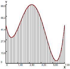
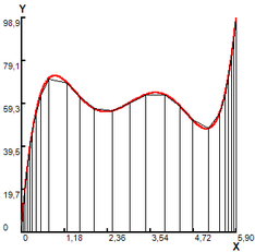
The function is numerically integrated in the interval ${\textstyle \left[0,\,4.2\right]}$ , with the partitions indicated in ${\textstyle NT}$ subintervals, all with the same upper base length. The results are shown in figure 1, and are presented in table 1.

In Figure 1(a), a grid with ${\textstyle NT=}$${\displaystyle 1}$fractal segment with an upper base ${\textstyle r=}$${\displaystyle 4.21}$ is superimposed on the interval ${\textstyle \left[0,\,4.2\right]}$ . The resulting area of 7.464 is a first approximation to the area of the region (table 1, case a,). In order to improve it, in Figure 1 (b) a variation is made, partitioning the curve with 3 fractal segments with an upper base ${\textstyle r=}$${\displaystyle 2.105}$, for a calculated total area of 38,195, with which a new coating of the R region (table 1, case b,) is formed. In Figure 1(c), a variation is presented, partitioning the curve with 9 fractal segments with an upper base ${\textstyle r=}$${\displaystyle 1.052}$ for a calculated total area of 51.221 (table 1, case c). In Figure 1 (d) a last variation is made by partitioning the curve with 21 fractal segments with an upper base ${\textstyle r=}$${\displaystyle 0.526}$. The integral of the curve is calculated by adding the area of the subintervals and equal to 54.306 (table 1, case d).

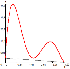
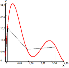
(1) Iter. 1, NT=1, r= 4.21	(2) Iter. 2. NT=3, r= 2.105
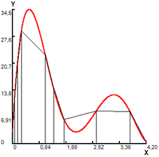
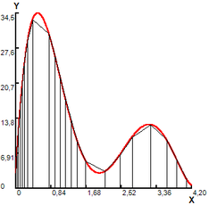
(3) Iter. 3, NT=9, r= 1.052	(4) Iter. 4, NT=21, r= 0.526

Figure 1. Area calculated by modified trapezoid rule.

Case a: ${\textstyle {\mathit {\boldsymbol {r}}}=}$${\displaystyle {\boldsymbol {4}}.{\boldsymbol {211}}}$
Area	${\displaystyle {\mathit {\boldsymbol {h}}}_{\mathit {\boldsymbol {1}}}}$	${\displaystyle {\mathit {\boldsymbol {h}}}_{\mathit {\boldsymbol {0}}}}$	${\displaystyle {\mathit {\boldsymbol {f}}}_{\mathit {\boldsymbol {1}}}}$	${\displaystyle {\mathit {\boldsymbol {f}}}_{\mathit {\boldsymbol {0}}}}$	${\displaystyle {{\mathit {\boldsymbol {h}}}{\mathit {\boldsymbol {=}}}{\mathit {\boldsymbol {h}}}}_{\mathit {\boldsymbol {1}}}-}$${\displaystyle {\mathit {\boldsymbol {h}}}_{\mathit {\boldsymbol {0}}}}$	${\displaystyle {\mathit {\boldsymbol {A=}}}{\frac {{\mathit {\boldsymbol {h}}}\left({\mathit {\boldsymbol {f}}}_{\mathit {\boldsymbol {0}}}{\mathit {\boldsymbol {+}}}{\mathit {\boldsymbol {f}}}_{\mathit {\boldsymbol {1}}}\right)}{\mathit {\boldsymbol {2}}}}}$
A1	4.2	0	0.553	3	4.2	7.464
Case b: ${\textstyle {\mathit {\boldsymbol {r}}}=}$${\displaystyle {\boldsymbol {2}}.{\boldsymbol {105}}}$
A1	0.151	0	20.282	3	0,151	1.757
A2	1.557	0.151	7.373	20.282	1.406	19.453
A3	3.656	1.557	8.806	7.373	2.098	16.981
Total						38.195
Case c: ${\textstyle {\mathit {\boldsymbol {r}}}=}$${\displaystyle {\boldsymbol {1}},{\boldsymbol {052}}}$
A1	0.067	0	11.729	3	0.067	0.493
A2	0.152	0.067	20.370	11.729	0.085	1.364
A3	0.28	0.152	29.007	20.370	0.128	3.160
A4	1.032	0.280	22.906	29.007	0.751	19.519
A5	1.284	1.032	14.468	22.906	0.252	4.727
A6	1.617	1.284	6.2416	14.468	0.332	3.448
A7	2.636	1.617	8.4341	6.2416	1.018	7.477
A8	3.689	2.636	8.2926	8.4341	1.052	8.806
A9	4.186	3.689	0.6556	8.2926	0.497	2.223
Total						51.221
Case d: ${\textstyle {\mathit {\boldsymbol {r}}}=}$${\displaystyle {\boldsymbol {0}}.{\boldsymbol {526}}}$
A1	0.032	0	7.394	3	0.032	0.166
A2	0.067	0.032	11.729	7.394	0.035	0.334
A3	0.107	0.067	16.114	11.729	0.040	0.556
A4	0.153	0.107	20.456	16.114	0.046	0.841
A5	0.209	0.153	24.811	20.456	0.056	1.267
A6	0.282	0.209	29.106	24.811	0.073	1.967
A7	0.405	0.282	33.336	29.106	0.123	3.840
A8	0.795	0.405	30.414	33.336	0.390	12.431
A9	0.934	0.795	26.208	30.414	0.139	3.935
A10	1.058	0.934	21.979	26.208	0.124	3.011
A11	1.182	1.058	17.756	21.979	0.123	2.463
A12	1.314	1.182	13.553	17.756	0.131	2.066
A13	1.466	1.314	9.403	13.553	0.151	1.744
A14	1.669	1.466	5.398	9.403	0.202	1.502
A15	2.132	1.669	3.333	5.398	0.462	2.021
A16	2.484	2.132	6.568	3.333	0.351	1.742
A17	2.783	2.484	10.141	6.568	0.298	2.498
A18	3.219	2.783	12.569	10.141	0.435	4.951
A19	3.602	3.219	9.593	12.569	0.382	4.244
A20	3.840	3.602	5.728	9.593	0.237	1.823
A21	4.076	3.840	1.854	5.728	0.236	0.894
Total						54.306

4.1 Calculating fractal dimension

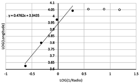
Next, the fractal dimension of the function (9), obtained with the trapezoid rule modified method, is calculated by dividing the curve with fractal segments, results recorded in Table 2, and represented in Figure 2.

In table 2, the slope ${\textstyle m}$ of the regression line that makes up the points ${\textstyle \left(Log\left(1/r\right),\,Log\left(Longitude\right)\right)}$ is calculated. ${\textstyle m}$is an estimate of the fractal dimension of the area under study.

Iter.	Fig	r	NI	${\displaystyle {\mathit {\boldsymbol {Longitude=r.NI}}}}$	${\displaystyle {\mathit {\boldsymbol {LOG(1/r)}}}}$	${\displaystyle {\mathit {\boldsymbol {LOG(Longitude)}}}}$
1	1(a)	4.211	1	4.211	-0,624	0,624
2	1(b)	2.105	3	6.317	-0,323	0,800
3	1(c)	1.058	9	9.475	-0,022	0,976
4	1(d)	0.526	21	11.055	0,278	1,043
5	-	0.2632	43	11.318	0,579	1,053
6	-	0.1312	86	11.318	0,880	1,053
7	-	0.0658	171	11.252	1,181	1,051

Table 2. Fractal dimension partitioning the curve using fractal segments.

Note that the results are shown with three additional iterations.

The fractal dimension is a parameter that characterizes the sinuous or irregular of an object. For the case under study. The fractal dimension determines the variability of the results in the different iterations. This means that when there is no variability, an error is entered into the calculations.

Note that the critical point of the Figure 2 was reached in iteration 4, from which no significant differences can be seen. For that reason, the fractal dimension calculated, using the least squares method, was delimited between 1 to 4 iterations, to eliminate the error due to invariability of the results in the interactions of 5 to 7. The result was rounded to 3 decimals, considering that the error obtained by the adjustment with least squares is in this range.

The slope ${\textstyle m}$ of the regression line is an estimate of the fractal dimension of the curve under study. With respect to the topological dimension ${\textstyle {(D}_{top})}$ of a line, the number of dimensions needed to fix a point on the line is 1. And because the fractional dimension ${\textstyle {(D}_{frac})}$ must be larger than its dimension topological, this is calculated as ${\textstyle {D}_{frac}=}$${\displaystyle {D}_{top}+m=1+m.}$The calculation shows a measure of the fractal dimension of the curve with a value of 1.476, which means that it is a curve with a medium degree of fluctuation.

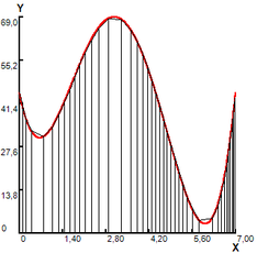
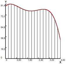
The previous function is integrated in the same interval ${\textstyle \left[a,b\right]}$ , with the partitions indicated in ${\textstyle n}$ subintervals, all of the same length ${\textstyle h=}$${\displaystyle (b-a)/n}$, results reported in table 3 and represented in figure 3.

In Figure 3(a), a grid with 1 trapezium in the interval ${\textstyle \left[0,\,4.2\right]}$ is superimposed on the region. The resulting area of 7.477, is a first approximation to the area of the region. In order to improve it, in Figure 3(b), a variation is made with 3 trapezoids in the intervals for a total calculated area of 32.502, with which forms a new superimposed of the R region. In Figure 3(c), a variation with 9 trapezoids is presented for a total calculated area of 52.281. In Figure 3(d), a last variation is made with 21 trapezoids. The approximate area under the curve is calculated by adding the area of the trapezoids and equal to 54.490 (table 4).

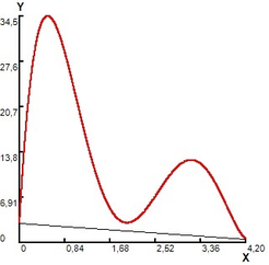
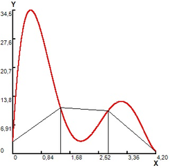
(1) n=1, h=4.2	(2) n=3, h=1.4
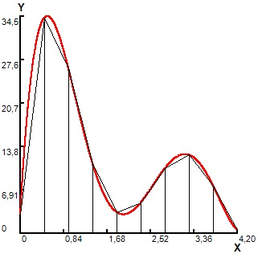
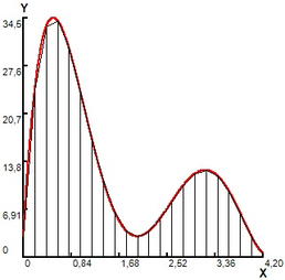
(3) n=9, h=0.466,	(4) n=21, h=0.2

Figure 3. Area calculating by trapezoid rule equiespaced.

Case a: ${\textstyle {\mathit {\boldsymbol {r}}}{\boldsymbol {=0.200}}}$
Area	${\displaystyle {\mathit {\boldsymbol {h}}}_{\mathit {\boldsymbol {1}}}}$	${\displaystyle {\mathit {\boldsymbol {h}}}_{\mathit {\boldsymbol {0}}}}$	${\displaystyle {\mathit {\boldsymbol {f}}}_{\mathit {\boldsymbol {1}}}}$	${\displaystyle {\mathit {\boldsymbol {f}}}_{\mathit {\boldsymbol {0}}}}$	${\displaystyle {{\mathit {\boldsymbol {h}}}{\mathit {\boldsymbol {=}}}{\mathit {\boldsymbol {h}}}}_{\mathit {\boldsymbol {1}}}-}$${\displaystyle {\mathit {\boldsymbol {h}}}_{\mathit {\boldsymbol {0}}}}$	${\displaystyle {\mathit {\boldsymbol {A=}}}{\frac {{\mathit {\boldsymbol {h}}}\left({\mathit {\boldsymbol {f}}}_{\mathit {\boldsymbol {0}}}{\mathit {\boldsymbol {+}}}{\mathit {\boldsymbol {f}}}_{\mathit {\boldsymbol {1}}}\right)}{\mathit {\boldsymbol {2}}}}}$
A1	0.200	0.00	24.176	3.000	0.2	2.717
A2	0.400	0.200	33.228	24.176	0.2	5.740
A3	0.600	0.400	34.187	33.228	0.2	6.741
A4	0.800	0.600	30.279	34.187	0.2	6.446
A5	1.000	0.800	24.000	30.279	0.2	5.427
A6	1.200	1.00	17.192	24.000	0.2	4.119
A7	1.400	1.200	11.124	17.192	0.2	2.831
A8	1.600	1.400	6.563	11.124	0.2	1.768
A9	1.800	1.600	3.855	6.563	0.2	1.041
A10	2.000	1.800	3.000	3.855	0.2	0.685
A11	2.200	2.000	3.728	3.000	0.2	0.672
A12	2.400	2.200	5.580	3.728	0.2	0.930
A13	2.600	2.400	7.979	5.580	0.2	1.356
A14	2.800	2.600	10.311	7.979	0.2	1.829
A15	3.000	2.800	12.000	10.311	0.2	2.231
A16	3.200	3.000	12.584	12.000	0.2	2.458
A17	3.400	3.200	11.796	12.584	0.2	2.438
A18	3.600	3.400	9.635	11.796	0.2	2.143
A19	3.800	3.600	6.447	9.635	0.2	1.608
A20	4.000	3.800	2.999	6.447	0.2	0.944
A21	4.200	4.00	0.560	2.999	0.2	0.356
Total						54.490

The area of the ${\textstyle R}$ region bounded by the function (9) is compared by the standard simple trapezoid rule, partitioning the curve with fractal segments.

Method	Result	${\textstyle {\mathit {\boldsymbol {E}}}{\mathit {\boldsymbol {RP=}}}{\frac {\left|{\mathit {\boldsymbol {A}}}^{\mathit {\boldsymbol {\ast }}}{\mathit {\boldsymbol {-A}}}\right|}{\mathit {\boldsymbol {A}}}}}$*100
Exact Area	53.212
Our trapezoid rule method for fractally (unequally) spaced data	54.306	2.014
Trapezoid rule for equallly spacing data	54.490	2.345

The value of the function integral (9) used as a reference is ${\textstyle {\mathit {\boldsymbol {A}}}^{\mathit {\boldsymbol {\ast }}}=}$${\displaystyle 53.212}$. Table 4 presents the results obtained, comparing the values of the integral of the curve studied, the relative percentage error (ERP). It is concluded that both methods are equally comparable

Next, the validation of the proposed method is presented, with the following three polynomial functions, all with different degrees of irregularity or fluctuation.

Polynomial functions
${\displaystyle y={x}^{4}-13{x}^{3}+49{x}^{2}-49x+45}$	(10)
${\displaystyle y={\left(x-3\right)}^{5}-8{\left(x-3\right)}^{3}+10\left(x-3\right)+60}$	(11)
${\displaystyle y=-3{x}^{4}+20{x}^{3}-41{x}^{2}+22x+88}$	(12)

The polynomial functions (10), (11) and (12) will be integrated in the intervals ${\textstyle \left[0,\,7\right]}$ , ${\textstyle \left[0,\,5.9\right]}$ and ${\textstyle \left[0,\,4\right]}$ . The exact areas are 274.869, 349.230 and 318.976. Dividing the functions using fractal procedure, in the iteration number 5, there are 41, 24 and 19 segments respectively.

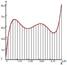
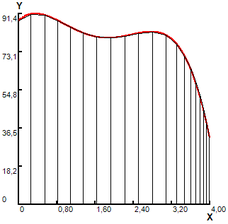
Figure 4 shows the partitions of the areas of the curves under study, using equally spaced data in the first case, and unequally spaced in the second.

Trapezoid rule equally spaced	Trapezoid rule fractally spaced
(1) Function (10), NI = 41 equispaced.	(2) Function (10), NI=41 unequally spaced
(3) Function (11), NI=24 equispaced	(4) Function (11), NI= 24 unequally spaced
(5) Function (12), NI=19 equispaced	(6) Function (12), NI=19 unequally spaced

Figure 4. Intervals equispaced and not equispaced for other functions.

Tables 6, 7 and 8 show the calculation of the integral and fractal dimension of the polynomial functions under study (10), (11) and (12) respectively.

Iter	${\displaystyle {\mathit {\boldsymbol {r}}}}$	${\displaystyle {\mathit {\boldsymbol {NI}}}}$	Area	${\displaystyle {\mathit {\boldsymbol {Longitude=r.NI}}}}$	${\displaystyle {\mathit {\boldsymbol {LOG(1/r)}}}}$	${\displaystyle {\mathit {\boldsymbol {LOG(Longitude)}}}}$
1	7.000	1	315.000	7.000	-0.845	0.845
2	3.500	4	302.463	14.000	-0.544	1.146
3	1.750	8	287.793	14.000	-0.243	1.146
4	0.875	20	277.548	17.500	0.057	1.243
5	0.437	41	274.791	17.937	0.359	1.253
6	0.218	83	274.832	18.156	0.660	1.259
7	0.109	165	274.699	18.046	0.961	1.256

Table 6. Fractal dimension, polynomial function ${\textstyle y=}$${\displaystyle {x}^{4}-13{x}^{3}+49{x}^{2}-49x+45}$.

Iter	${\displaystyle {\mathit {\boldsymbol {r}}}}$	${\displaystyle {\mathit {\boldsymbol {NT}}}}$	Area	${\displaystyle {\mathit {\boldsymbol {Longitude=r.NT}}}}$	${\displaystyle {\mathit {\boldsymbol {LOG(1/r)}}}}$	${\displaystyle {\mathit {\boldsymbol {LOG(Longitude)}}}}$
1	8.218	1	300.898	8.218	-0.914	0.914
2	4.109	2	270.113	8.218	-0.613	0.914
3	2.054	5	339.050	10.273	-0.312	1.011
4	1.027	11	346.767	11.300	-0.011	1.053
5	0.513	24	348.170	12.327	0.289	1.090
6	0.256	48	347.850	12.327	0.590	1.090
7	0.128	96	348.443	12.327	0.891	1.090

Table 7. Fractal dimension, polynomial function ${\textstyle y=}$${\displaystyle {\left(x-3\right)}^{5}-8{\left(x-3\right)}^{3}+10\left(x-3\right)+60}$

Iter	${\displaystyle {\mathit {\boldsymbol {r}}}}$	${\displaystyle {\mathit {\boldsymbol {NT}}}}$	Area	${\displaystyle {\mathit {\boldsymbol {Longitude=r.NT}}}}$	${\displaystyle {\mathit {\boldsymbol {LOG(1/r)}}}}$	${\displaystyle {\mathit {\boldsymbol {LOG(Longitude)}}}}$
1	4.693	1	239.831	4.693	-0.671	0.671
2	2.346	2	294.116	4.693	-0.370	0.671
3	1.173	4	306.375	4.693	-0.069	0.671
4	0.586	9	315.353	5.279	0.231	0.722
5	0.293	19	318.351	5.573	0.532	0.746
6	0.146	38	318.650	5.573	0.833	0.746
7	0.073	76	318.942	5.573	1.134	0.746

Table 8. Fractal dimension, polynomial function ${\textstyle y=}$${\displaystyle -3{x}^{4}+20{x}^{3}-41{x}^{2}+22x+88}$

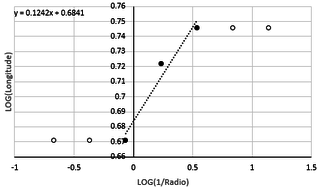
Next, the fractal dimension of the functions (10, 11 and 12), are calculated by dividing the curve with fractal segments, results are represented in Figures 5, 6 and 7.

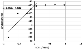
Figure 5. Regression line, function (10).

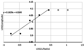
Figure 6. Regression line, function (11).

Note that in figures 5, 6 and 7 the critical points were reached in iterations 4, 5 and 5 respectively, from which no significant differences can be seen. For that reason, the fractal dimension calculated, using the least squares method, was delimited between 1 to 4, 1 to 5, 3 to 5 iterations respectively, to eliminate the error due to invariability of the results in the interactions of 5 to 7 (Figure 5), 6 to 7 (Figure 6), 1 to 2 and 6 to 7 (Figure 7), respectively.

Table 9 presents the results obtained, comparing the values of the integral of the curve studied, the relative percentage error (ERP), using the methods Trapezoid rule standard and Trapezoid rule modified, partitioning the curve with fractal segments.

As evidenced in Table 9, the method proposed in this article, dividing the trapezoids from the fractal fragmentation of its upper side, presents results comparable with those obtained with the traditional composite trapezoid method, in which the lower sides of the sets are equally spaced.

Function	Exact Area	${\displaystyle {\mathit {\boldsymbol {NI}}}}$	Area equally spaced	${\displaystyle {\mathit {\boldsymbol {ERP}}}}$	Area fractally spaced	${\displaystyle {\mathit {\boldsymbol {ERP}}}}$	Fractal Dim.
(10)	274.869	41	275.340	0.171	274.791	0.028	1.396
(11)	349.230	24	349.040	0.054	348.170	0.304	1.162
(12)	318.976	19	318.430	0.171	318.351	0.196	1.124

Table 9. Area comparison.

With respect to the fractal dimension of the curves studied, their values are 1.396, 1.162 and 1.124 respectively, an index that effectively reveals their degree of fluctuation. The polynomial function (10) has a maximum point over two deep basins at different slopes. With respect to (10), the direction of the function (11) changes more smoothly between its two points of maximum and minimum (all of them almost at the same level), respectively. Finally (12) it is the function with smoother changes, with negative bias to the left of the study interval.

5. Conclusions

In the present paper the working hypothesis was validated: The degree of fluctuation of a function is calculated using fractal dimension method. The fractal segments obtained also may be used to calculate the area under the curve, integrating the function using standard trapezoid rule, with fractally spaced data, from which other relevant observations may be obtained from its analysis, such as:

(1) The great advantage of the proposed method is that it unifies the calculation of the numerical integration of a function, together with its corresponding fractal dimension, a task not performed with conventional numerical integration methods.

(2) To calculate the fractal dimension, the standard method uses a compass that with a specific radius, an arc is drawn to find the point that intercepts the curve. In this article a compass was not used, because an algorithm was developed to find the point that intercepts the curve studied with a specific radius.

(3) The fractal dimension is a quantitative estimator of spatial complexity.

(4) It is confirmed that the fractal dimension satisfactorily describes the degree of irregularity of a function, an impossible measure to make using Euclidean (classical) geometry that is limited to regular shapes.

(5) The calculation of the fractal dimension of the studied surface cannot be obtained exactly but estimated, being very sensitive to numerical or experimental noise, and particularly to the limitations in the amount of data

This work was supported by the Agencia de Educación Superior de Medellín (SAPIENCIA) under the specific agreement celebrated with the Institución Universitaria Pascual Bravo. The project is part of the Energy System Doctorate Program of the Universidad Nacional de Colombia, Sede Medellín, Facultad de Minas.

Conflicts of Interest: The authors declare no conflict of interest.

References

[1] M.F. Barnsley, R.L. Devaney, B.B. Mandelbrot, H.-O. Peitgen, D. Saupe, R.F. Voss, The Science of Fractal Images, Springer New York, New York, NY, 1988. doi:10.1007/978-1-4612-3784-6.

[2] S.H. Strogatz, Nonlinear Dynamics and Chaos, CRC Press, 2018. doi:10.1201/9780429492563.

[3] G.A. Losa, Fractals and Their Contribution to Biology and Medicine, Medicographia. 34 (2012) 365–374.

[4] T.A. Garcia, G.A. Tamura Ozaki, R.C. Castoldi, T.E. Koike, R.C. Trindade Camargo, J.C. Silva Camargo Filho, Fractal dimension in the evaluation of different treatments of muscular injury in rats, Tissue Cell. 54 (2018) 120–126. doi:10.1016/j.tice.2018.08.014.

[5] J.O. Rodríguez V, S.E. Prieto B, S.C. Correa H, M.Y. Soracipa M, L.R. Mendez P, H.J. Bernal C, N.C. Hoyos O, L.P. Valero, A. Velasco R, E. Bermudez, Nueva metodología de evaluación del Holter basada en los sistemas dinámicos y la geometría fractal: confirmación de su aplicabilidad a nivel clínico, Rev. La Univ. Ind. Santander. Salud. 48 (2016) 27–36. doi:10.18273/revsal.v48n1-2016003.

[6] N. Popovic, M. Radunovic, J. Badnjar, T. Popovic, Fractal dimension and lacunarity analysis of retinal microvascular morphology in hypertension and diabetes, Microvasc. Res. 118 (2018) 36–43. doi:10.1016/j.mvr.2018.02.006.

[7] J. de D. Hernández Velázquez, S. Mejía-Rosales, A. Gama Goicochea, Fractal properties of biophysical models of pericellular brushes can be used to differentiate between cancerous and normal cervical epithelial cells, Colloids Surfaces B Biointerfaces. 170 (2018) 572–577. doi:10.1016/j.colsurfb.2018.06.059.

[8] P. Moon, J. Muday, S. Raynor, J. Schirillo, C. Boydston, M.S. Fairbanks, R.P. Taylor, Fractal images induce fractal pupil dilations and constrictions, Int. J. Psychophysiol. 93 (2014) 316–321. doi:10.1016/j.ijpsycho.2014.06.013.

[9] B.B. Mandelbrot, R.L. Hudson, The (mis) Behaviour of Markets: A Fractal View of Risk, Ruin and Reward, Profile Books, London, 2004.

[10] R. Kumar, P.N. Chaubey, On the design of tree-type ultra wideband fractal Antenna for DS-CDMA system, J. Microwaves, Optoelectron. Electromagn. Appl. 11 (2012) 107–121. doi:10.1590/S2179-10742012000100009.

[11] Y.-J. Ma, M.-Y. Zhai, Fractal and multi-fractal features of the broadband power line communication signals, Comput. Electr. Eng. 72 (2018) 566–576. doi:10.1016/j.compeleceng.2018.01.025.

[12] D. Ye, M. Dai, Y. Sun, W. Su, Average weighted receiving time on the non-homogeneous double-weighted fractal networks, Phys. A Stat. Mech. Its Appl. 473 (2017) 390–402. doi:10.1016/j.physa.2017.01.013.

[13] H. Tabares-Ospina, F. Angulo, M. Osorio, A new methodology to analyze the dynamic of daily power demand with attractors into the Mandelbrot set, Fractals. 28 (2020) 2050003–1, 2050003–9. doi:10.1142/S0218348X20500036.

[14] J. Colomer, A. Naranjo, V. Janvier, T. Mossi, Evaluation of fractal dimension effectiveness for damage detection in retinal background, J. Comput. Appl. Math. 337 (2018) 341–353.

[15] F. Guosheng, X. Weimin, Y. Feng, Y. Yi, W. Yuan, Surface fractal dimension of bentonite affected by long-term corrosion in alkaline solution, Appl. Clay Sci. 175 (2019) 94–101.

[16] R. Swain, S. Roy, P. Mukherjee, B. Sawkar, Fractal dimension and its translation into a model of gold spatial proxy, Ore Geol. Rev. 110 (2019) 1–10.

[17] X. Yongfu, Fractal dimension of demolition waste fragmentation and its implication of compactness, Powder Technol. 339 (2018) 922–929.

[18] E. Martos, F. Lapuerta, M. Expósito, Juan. Sanmiguel-Rojas, Overestimation of the fractal dimension from projections of soot agglomerates, Powder Technol. 311 (2017) 528–536.

[19] F. Yang, X. Zhang, R. Ma, S. Yang, X, Wand, Fractal dimension of concrete meso-structure based on X-ray computed tomography, Powder Technol. 350 (2019) 91–99.

[20] J. Jiménez, A. Anzola, J. Jimenez-Triana, Pedestrian counting estimation based on fractal dimension, Heliyon. (2019). doi:10.1016/j.heliyon.2019. e01449.

[21] L. Chen, Y. Huang, Modeling growth curve of fractal dimension of urban form of Beijing, Physica A. 523 (2019) 1038–1056.

[22] E. Pashminehazar, R. Kharaghani, A. Tsotsas, Determination of fractal dimension and prefactor of agglomerates with irregular structure, Powder Technol. 343 (2019) 765–774.

[23] M.S.M. Navascués, Numerical integration of affine fractal functions, J. Comput. Appl. Math. 252 (2013) 169–176.

[24] D. Raghavendra, B. Dutt, Computing Fractal Dimension of Signals using Multiresolution Boxcounting Method, Int. J. Inf. Math. Sci. (2010) 50–65.

[25] R. Chapra, S. Canale, Numerical methods for engineers, Fifty, The McGraw-Hill Companies, Mexico, 2006.

[26] S. Mamun-Ur-Rashid, M. Hossain, M. Parvin, Numerical Integration Schemes for Unequal Data Spacing, Am. J. Appl. Math. 2 (2017) 48–56.

[27] K. Mathews, J. Fink, Numerical methods using MATLAB, third, Madrid, 2000.

[28] R. Malmquist, J. Stricharts, Numerical integration for fractal measures, J. Fractal Geom. 5 (2018) 165–226.

[29] G. Ranjan, S. Mishra, J, Palai, Analysing roughness of surface through fractal dimension: A review, Image Vis. Comput. 89 (2019) 21–34.