(Created page with "==1 Title, abstract and keywords<!-- Your document should start with a concise and informative title. Titles are often used in information-retrieval systems. Avoid abbreviatio...") |
m (Move page script moved page Draft Samper 881068008 to Onate et al 2007g) |
||
| (One intermediate revision by one other user not shown) | |||
| Line 1: | Line 1: | ||
| − | == | + | == Abstract == |
| − | + | This paper shows applications of a recently developed thin shell element adequate for the analysis of membrane and inflatable structures. The element is a three node triangle with only translational degrees of freedom that uses the configuration of the three adjacent elements to evaluate the strains in terms of the nodal displacements only. This allows to compute (constant) bending strains and (linear) membrane strains using a total Lagrangian formulation. Several examples, including inflation and deflation of membranes and some practical applications to the analysis, design and construction of membrane structures formed by low pressure inflatable tubes are presented. | |
| − | + | '''Keywords''' shell elements, rotation free shell triangle, membrane structures, inflatable structures, low pressure inflatable tubes | |
| + | ==1 Introduction== | ||
| + | Inflatable structures have unique features. Because of their foldability and air- or helium pneumatic stabilisation they cannot be compared to any classical structural concepts. | ||
| + | Inflatable structures have become increasingly popular in recent years for a wide range of applications in architecture, civil engineering, aeronautic and airspace situations. | ||
| − | + | The use of inflatable structures can be found in temporary and/or foldable structures to cover large spaces or to support other elements, in permanent roofs or shelters with a high degree of transparency, in mobile buildings as temporary housing in civil logistic missions (e.g. environmental disasters and rescue situations), in the construction of tunnels and dams, in antennas for both ground and aerospace applications, as well as in extremely light airship structures among other uses <span id='citeF-1'></span> <span id='citeF-11'></span>[[#cite-1|[1]]-[[#cite-11|11]]]. | |
| − | + | Some efforts have been made in the past years to develop inflated structures formed by assembly of high pressure tubes. The obvious disadvantages of these structures are the design of the joints and their big vulnerability to air losses. In general, high pressure inflated structures are difficult to maintain and repair and have a high cost. | |
| + | Inflatable structures formed by an assembly of self-supported low pressure tubular membrane elements are ideal to cover large space areas. They also adapt easily to any design shape and have minimal maintenance requirements, other than keeping a constant low internal pressure accounting for the air losses through the material pores and the seams. | ||
| − | + | The simulation of the inflation of membrane structures is normally performed with membrane finite elements, i.e. no bending stiffness included. The formulation of such elements is simple as they only require <math display="inline">C^{0}</math> continuity <span id='citeF-12'></span>[[#cite-12|[12]]], in contrast with elements based on thin shell theory where <math display="inline">C^{1}</math> continuity implies important obstacles <span id='citeF-13'></span>[[#cite-13|[13]]] in the development of conforming elements. Triangular elements are naturally preferred as they can easily adapt to arbitrary geometries and due to the robustness of the associated mesh generators. | |
| − | + | Membrane structures components have some, although small, bending stiffness that in most cases is disregarded. However in many applications it is convenient to include bending energy in the model due to the important regularization effect it introduces. Shell elements are typically more complex and expensive due the increase in degrees of freedom (rotations) and integration points (through the thickness). In the last few years shell elements without rotation degrees of freedom have been developed <span id='citeF-14'></span> <span id='citeF-22'></span>[[#cite-14|[14]]-[[#cite-22|22]]], which make shell elements more efficient for both implicit and explicit integration schemes. | |
| + | When only the final configuration of the membrane is of interest implicit schemes are normally used, including special algorithms due to the lack of stiffness of the membrane when no tensile stresses are yet present. When the inflation/deflation process is of interest, the explicit integration of the momentum equations is largely preferred. Modeling of complex deformation with constant strain shell triangles, such as those occuring in the inflation-deflation process of inflatable membranes accounting for frictional contact conditions typically require fine discretizations. These type of simulations can be time consuming due to the time increment limitations. In this paper a rotation-free triangular shell element with similar convergence properties to the linear strain triangle, but without its drawbacks, is used. | ||
| − | + | The outline of this chapter is as follows. Next two section summarizes the rotation-free shell triangle used. [[#4 Aeroelastic Analysis|Section 4]] summarices the procedure for aeroelastic analysis. [[#5 Examples|Section 5]] presents examples of application to the analysis of inflatable membranes. The paper concludes with practical examples inflatable structures formed by low pressure inflatable tubes designed and analyzed using the technology described in the paper. Finally [[#6 Concluding Remarks|Section 6]] summarizes some conclusions. | |
| − | + | ==2 Formulation of the Rotation Free Shell Triangle== | |
| − | + | ===2.1 Shell Kinematics=== | |
| − | + | A summary of the most relevant hypothesis related to the kinematic behaviour of a thin shell are presented. Further details may be found in the wide literature dedicated to this field <span id='citeF-21'></span> <span id='citeF-23'></span>[[#cite-21|[21]]-[[#cite-23|23]]]. | |
| − | + | Consider a shell with undeformed middle surface occupying the domain <math display="inline">\Omega ^{0}</math> in <math display="inline">R^{3}</math> with a boundary <math display="inline">\Gamma ^{0}</math>. At each point of the middle surface a thickness <math display="inline">h^{0}</math> is defined. The positions <math display="inline">\mathbf{x}^{0}</math> and <math display="inline">\mathbf{x}</math> of a point in the undeformed and the deformed configurations can be respectively written as a function of the coordinates of the middle surface <math display="inline">{\boldsymbol \varphi }</math> and the normal <math display="inline">\mathbf{t}_{3}</math> at the point as | |
| − | + | {| class="formulaSCP" style="width: 100%; text-align: left;" | |
| + | |- | ||
| + | | | ||
| + | {| style="text-align: left; margin:auto;width: 100%;" | ||
| + | |- | ||
| + | | style="text-align: center;" | <math>\mathbf{x}^{0}\left( \xi _{1},\xi _{2},\zeta \right) ={\boldsymbol \varphi }^{0}\left( \xi _{1},\xi _{2}\right) +\lambda \mathbf{t}_{3}^{0}</math> | ||
| + | | style="width: 5px;text-align: right;white-space: nowrap;" | (1) | ||
| + | |- | ||
| + | | style="text-align: center;" | <math> \mathbf{x}\left( \xi _{1},\xi _{2},\zeta \right) ={\boldsymbol \varphi }\left( \xi _{1},\xi _{2}\right) +\zeta \lambda \mathbf{t}_{3}</math> | ||
| + | | style="width: 5px;text-align: right;white-space: nowrap;" | (2) | ||
| + | |} | ||
| + | |} | ||
| + | where <math display="inline">\xi _{1},\xi _{2}</math> are arc-length curvilinear principal coordinates defined over the middle surface of the shell and <math display="inline">\zeta </math> is the distance from the point to the middle surface in the undeformed configuration. The product <math display="inline">\zeta \lambda </math> is the distance from the point to the middle surface measured on the deformed configuration. The parameter <math display="inline">\lambda </math> relates the thickness at the present and initial configurations as: | ||
| − | + | {| class="formulaSCP" style="width: 100%; text-align: left;" | |
| + | |- | ||
| + | | | ||
| + | {| style="text-align: left; margin:auto;width: 100%;" | ||
| + | |- | ||
| + | | style="text-align: center;" | <math>\lambda =\frac{h}{h^{0}}</math> | ||
| + | |} | ||
| + | | style="width: 5px;text-align: right;white-space: nowrap;" | (3) | ||
| + | |} | ||
| − | + | This approach implies a constant strain in the normal direction. Parameter <math display="inline">\lambda </math> will not be considered as an independent variable and will be computed from purely geometrical considerations (''isochoric'' behaviour) via a staggered iterative update. Besides this, the usual plane stress condition of thin shell theory will be adopted. | |
| − | + | A convective system is computed at each point as | |
| − | + | {| class="formulaSCP" style="width: 100%; text-align: left;" | |
| + | |- | ||
| + | | | ||
| + | {| style="text-align: left; margin:auto;width: 100%;" | ||
| + | |- | ||
| + | | style="text-align: center;" | <math>\mathbf{g}_{i}\left( \mathbf{\xi }\right) =\frac{\partial \mathbf{x}}{\partial \xi _{i}}\qquad i=1,2,3</math> | ||
| + | | style="width: 5px;text-align: right;white-space: nowrap;" | (4) | ||
| + | |- | ||
| + | | style="text-align: center;" | <math> \mathbf{g}_{\alpha }\left( \mathbf{\xi }\right) =\frac{\partial \left( \mathbf{\boldsymbol \varphi }\left( \xi _{1},\xi _{2}\right) +\zeta \lambda \mathbf{t}_{3}\right) }{\partial \xi _{\alpha }}={\boldsymbol \varphi }_{^{\prime }\alpha }+\zeta \left( \lambda \mathbf{t}_{3}\right) _{^{\prime }\alpha }\quad \alpha=1,2</math> | ||
| + | | style="width: 5px;text-align: right;white-space: nowrap;" | (5) | ||
| + | |- | ||
| + | | style="text-align: center;" | <math> \mathbf{g}_{3}\left( \mathbf{\xi }\right) =\frac{\partial \left( \mathbf{\boldsymbol \varphi }\left( \xi _{1},\xi _{2}\right) +\zeta \lambda \mathbf{t}_{3}\right) }{\partial \zeta }=\lambda \mathbf{t}_{3}</math> | ||
| + | | style="width: 5px;text-align: right;white-space: nowrap;" | (6) | ||
| + | |} | ||
| + | |} | ||
| − | + | This can be particularized for the points on the middle surface as | |
| − | + | {| class="formulaSCP" style="width: 100%; text-align: left;" | |
| + | |- | ||
| + | | | ||
| + | {| style="text-align: left; margin:auto;width: 100%;" | ||
| + | |- | ||
| + | | style="text-align: center;" | <math>\mathbf{a}_{\alpha } =\mathbf{g}_{\alpha }\left( \zeta=0\right) ={\boldsymbol \varphi }_{^{\prime }\alpha }</math> | ||
| + | | style="width: 5px;text-align: right;white-space: nowrap;" | (7) | ||
| + | |- | ||
| + | | style="text-align: center;" | <math> \mathbf{a}_{3} =\mathbf{g}_{3}\left( \zeta=0\right) =\lambda \mathbf{t}_{3}</math> | ||
| + | | style="width: 5px;text-align: right;white-space: nowrap;" | (8) | ||
| + | |} | ||
| + | |} | ||
| − | + | The covariant (first fundamental form) metric tensor of the middle surface is | |
| − | + | <span id="eq-9"></span> | |
| + | {| class="formulaSCP" style="width: 100%; text-align: left;" | ||
| + | |- | ||
| + | | | ||
| + | {| style="text-align: left; margin:auto;width: 100%;" | ||
| + | |- | ||
| + | | style="text-align: center;" | <math>a_{\alpha \beta }=\mathbf{a}_{\alpha }\cdot \mathbf{a}_{\beta } = {\boldsymbol \varphi }_{^{\prime }\alpha } \cdot {\boldsymbol \varphi }_{^{\prime }\beta } </math> | ||
| + | |} | ||
| + | | style="width: 5px;text-align: right;white-space: nowrap;" | (9) | ||
| + | |} | ||
| − | + | The Green-Lagrange strain vector of the middle surface points (membrane strains) is defined as | |
| − | + | {| class="formulaSCP" style="width: 100%; text-align: left;" | |
| + | |- | ||
| + | | | ||
| + | {| style="text-align: left; margin:auto;width: 100%;" | ||
| + | |- | ||
| + | | style="text-align: center;" | <math>{\boldsymbol \varepsilon }_{m}=[\varepsilon _{m_{11}},\varepsilon _{m_{12}},\varepsilon _{m_{12}}]^{T}</math> | ||
| + | |} | ||
| + | | style="width: 5px;text-align: right;white-space: nowrap;" | (10) | ||
| + | |} | ||
| − | + | with | |
| − | + | <span id="eq-11"></span> | |
| + | {| class="formulaSCP" style="width: 100%; text-align: left;" | ||
| + | |- | ||
| + | | | ||
| + | {| style="text-align: left; margin:auto;width: 100%;" | ||
| + | |- | ||
| + | | style="text-align: center;" | <math>\varepsilon _{m_{ij}}=\frac{1}{2}(a_{ij}-a_{ij}^{0}) </math> | ||
| + | |} | ||
| + | | style="width: 5px;text-align: right;white-space: nowrap;" | (11) | ||
| + | |} | ||
| + | The curvatures (second fundamental form) of the middle surface are obtained by | ||
| − | 2 | + | {| class="formulaSCP" style="width: 100%; text-align: left;" |
| + | |- | ||
| + | | | ||
| + | {| style="text-align: left; margin:auto;width: 100%;" | ||
| + | |- | ||
| + | | style="text-align: center;" | <math>\kappa _{\alpha \beta }=\frac{1}{2}\left( {\boldsymbol \varphi }_{^{\prime }\alpha }\cdot \mathbf{t}_{3^{\prime }\beta }+{\boldsymbol \varphi }_{^{\prime }\beta }\cdot \mathbf{t}_{3^{\prime }\alpha }\right) =- \mathbf{t}_{3}\cdot{\boldsymbol \varphi }_{{\prime }\alpha \beta }\quad , \quad \alpha ,\beta=1,2 </math> | ||
| + | |} | ||
| + | | style="width: 5px;text-align: right;white-space: nowrap;" | (12) | ||
| + | |} | ||
| − | + | The deformation gradient tensor is | |
| + | {| class="formulaSCP" style="width: 100%; text-align: left;" | ||
| + | |- | ||
| + | | | ||
| + | {| style="text-align: left; margin:auto;width: 100%;" | ||
| + | |- | ||
| + | | style="text-align: center;" | <math>\mathbf{F=} [{\boldsymbol x}_{{\prime }1},{\boldsymbol x}_{{\prime }2},{\boldsymbol x}_{{\prime }3}]=\left[ \begin{array}{ccc}{\boldsymbol \varphi }_{^{\prime }1}+\zeta \left( \lambda \mathbf{t}_{3}\right) _{^{\prime }1} & {\boldsymbol \varphi }_{^{\prime }2}+\zeta \left( \lambda \mathbf{t}_{3}\right) _{^{\prime }2} & \lambda \mathbf{t}_{3}\end{array} \right] </math> | ||
| + | |} | ||
| + | | style="width: 5px;text-align: right;white-space: nowrap;" | (13) | ||
| + | |} | ||
| + | The product <math display="inline">\mathbf{F}^{T}\mathbf{F=U}^{2}=\mathbf{C}</math> (where <math display="inline">\mathbf{U}</math> is the right stretch tensor, and <math display="inline">\mathbf{C}</math> the right Cauchy-Green deformation tensor) can be written as | ||
| + | <span id="eq-14"></span> | ||
| + | {| class="formulaSCP" style="width: 100%; text-align: left;" | ||
| + | |- | ||
| + | | | ||
| + | {| style="text-align: left; margin:auto;width: 100%;" | ||
| + | |- | ||
| + | | style="text-align: center;" | <math>\mathbf{U}^{2}=\left[ \begin{array}{ccc}a_{11}+2\kappa _{11}\zeta \lambda & a_{12}+2\kappa _{12}\zeta \lambda & 0\\ a_{12}+2\kappa _{12}\zeta \lambda & a_{22}+2\kappa _{22}\zeta \lambda & 0\\ 0 & 0 & \lambda ^{2}\end{array} \right] </math> | ||
| + | |} | ||
| + | | style="width: 5px;text-align: right;white-space: nowrap;" | (14) | ||
| + | |} | ||
| − | + | In the derivation of expression ([[#eq-14|14]]) the derivatives of the thickness ratio <math display="inline">\lambda _{^{\prime }a}</math> and the terms associated to <math display="inline">\zeta ^{2}</math> have been neglected. | |
| − | + | ||
| − | + | Equation ([[#eq-14|14]]) shows that <math display="inline">\mathbf{U}^{2}</math> is not a unit tensor at the original configuration for curved surfaces (<math display="inline">\kappa _{ij}^{0}\neq{0}</math>). The changes of curvature of the middle surface are computed by | |
| + | {| class="formulaSCP" style="width: 100%; text-align: left;" | ||
| + | |- | ||
| + | | | ||
| + | {| style="text-align: left; margin:auto;width: 100%;" | ||
| + | |- | ||
| + | | style="text-align: center;" | <math>\chi _{ij}=\kappa _{ij}-\kappa _{ij}^{0}</math> | ||
| + | |} | ||
| + | | style="width: 5px;text-align: right;white-space: nowrap;" | (15) | ||
| + | |} | ||
| + | Note that <math display="inline">\delta \chi _{ij}=\delta \kappa _{ij}</math>. | ||
| + | For computational convenience the following approximate expression (which is exact for initially flat surfaces) will be adopted | ||
| − | = | + | <span id="eq-16"></span> |
| + | {| class="formulaSCP" style="width: 100%; text-align: left;" | ||
| + | |- | ||
| + | | | ||
| + | {| style="text-align: left; margin:auto;width: 100%;" | ||
| + | |- | ||
| + | | style="text-align: center;" | <math>\mathbf{U}^{2}=\left[ \begin{array}{ccc}a_{11}+2\chi _{11}\zeta \lambda & a_{12}+2\chi _{12}\zeta \lambda & 0\\ a_{12}+2\chi _{12}\zeta \lambda & a_{22}+2\chi _{22}\zeta \lambda & 0\\ 0 & 0 & \lambda ^{2}\end{array} \right] </math> | ||
| + | |} | ||
| + | | style="width: 5px;text-align: right;white-space: nowrap;" | (16) | ||
| + | |} | ||
| + | This expression is useful to compute different Lagrangian strain measures. An advantage of these measures is that they are associated to material fibres, what makes it easy to take into account material anisotropy. It is also useful to compute the eigen decomposition of <math display="inline">\mathbf{U}</math> as | ||
| + | {| class="formulaSCP" style="width: 100%; text-align: left;" | ||
| + | |- | ||
| + | | | ||
| + | {| style="text-align: left; margin:auto;width: 100%;" | ||
| + | |- | ||
| + | | style="text-align: center;" | <math>\mathbf{U=}\sum _{\alpha=1}^{3}\lambda _{\alpha } \mathbf{r}_{\alpha }\otimes \mathbf{r}_{\alpha }</math> | ||
| + | |} | ||
| + | | style="width: 5px;text-align: right;white-space: nowrap;" | (17) | ||
| + | |} | ||
| + | where <math display="inline">\lambda _{\alpha }</math> and <math display="inline">\mathbf{r}_{\alpha }</math> are the eigenvalues and eigenvectors of <math display="inline">\mathbf{U}</math>. | ||
| − | + | The resultant stresses (axial forces and bending moments) are obtained by integrating across the original thickness the second Piola-Kirchhoff stress vector <math display="inline">{ \boldsymbol \sigma }</math> using the actual distance to the middle surface for evaluating the bending moments. This gives | |
| − | + | <span id="eq-18"></span> | |
| + | {| class="formulaSCP" style="width: 100%; text-align: left;" | ||
| + | |- | ||
| + | | | ||
| + | {| style="text-align: left; margin:auto;width: 100%;" | ||
| + | |- | ||
| + | | style="text-align: center;" | <math>{\boldsymbol \sigma }_{m}\equiv \lbrack N_{11},N_{22},N_{12}]^{T}=\int _{h^{0}}{\boldsymbol \sigma }d\zeta </math> | ||
| + | |} | ||
| + | | style="width: 5px;text-align: right;white-space: nowrap;" | (18) | ||
| + | |} | ||
| − | + | <span id="eq-19"></span> | |
| + | {| class="formulaSCP" style="width: 100%; text-align: left;" | ||
| + | |- | ||
| + | | | ||
| + | {| style="text-align: left; margin:auto;width: 100%;" | ||
| + | |- | ||
| + | | style="text-align: center;" | <math>{\boldsymbol \sigma }_{b}\equiv \lbrack M_{11},M_{22},M_{12}]^{T}=\int _{h^{0}}{\boldsymbol \sigma }\lambda \zeta d\zeta </math> | ||
| + | |} | ||
| + | | style="width: 5px;text-align: right;white-space: nowrap;" | (19) | ||
| + | |} | ||
| − | + | With these values the virtual work can be written as | |
| − | [ | + | <span id="eq-20"></span> |
| + | {| class="formulaSCP" style="width: 100%; text-align: left;" | ||
| + | |- | ||
| + | | | ||
| + | {| style="text-align: left; margin:auto;width: 100%;" | ||
| + | |- | ||
| + | | style="text-align: center;" | <math>\iint _{A^{0}}\left[ \delta{\boldsymbol \varepsilon }_{m}^{T}{\boldsymbol \sigma }_{m}+\delta{\boldsymbol \kappa }^{T}{\boldsymbol \sigma }_{b}\right] dA=\iint _{A^{0}}\delta \mathbf{u}^{T}\mathbf{t}dA </math> | ||
| + | |} | ||
| + | | style="width: 5px;text-align: right;white-space: nowrap;" | (20) | ||
| + | |} | ||
| − | [6] | + | where <math display="inline">\delta \mathbf{u}</math> are virtual displacements, <math display="inline">\delta{\boldsymbol \varepsilon }_{m}</math> is the virtual Green-Lagrange membrane strain vector, <math display="inline">\delta{\boldsymbol \kappa }</math> are the virtual curvatures and <math display="inline">\mathbf{t}</math> are the surface loads. Other load types can be easily included into ([[#eq-20|20]]). |
| − | -->== | + | |
| + | ===2.2 Constitutive Models=== | ||
| + | |||
| + | In order to treat non linear material behaviour at finite strains an adequate stress-strain pair must be used. The Hencky measures will be adopted here. The (logarithmic) strains are defined as | ||
| + | |||
| + | <span id="eq-21"></span> | ||
| + | {| class="formulaSCP" style="width: 100%; text-align: left;" | ||
| + | |- | ||
| + | | | ||
| + | {| style="text-align: left; margin:auto;width: 100%;" | ||
| + | |- | ||
| + | | style="text-align: center;" | <math>\mathbf{E}_{\ln }\mathbf{=}\left[ \begin{array}{ccc}\varepsilon _{11} & \varepsilon _{21} & 0\\ \varepsilon _{12} & \varepsilon _{22} & 0\\ 0 & 0 & \varepsilon _{33}\end{array} \right] =\sum _{\alpha=1}^{3}\ln \left( \lambda _{\alpha }\right) \mathbf{r}_{\alpha }\otimes \mathbf{r}_{\alpha } </math> | ||
| + | |} | ||
| + | | style="width: 5px;text-align: right;white-space: nowrap;" | (21) | ||
| + | |} | ||
| + | |||
| + | The use of a logarithmic strain measure reasonably allows to adopt an additive decomposition of elastic and non-linear (plastic) strain components as | ||
| + | |||
| + | <span id="eq-22"></span> | ||
| + | {| class="formulaSCP" style="width: 100%; text-align: left;" | ||
| + | |- | ||
| + | | | ||
| + | {| style="text-align: left; margin:auto;width: 100%;" | ||
| + | |- | ||
| + | | style="text-align: center;" | <math>\mathbf{E}_{\ln }\mathbf{=E}_{\ln }^{e}+\mathbf{E}_{\ln }^{p} </math> | ||
| + | |} | ||
| + | | style="width: 5px;text-align: right;white-space: nowrap;" | (22) | ||
| + | |} | ||
| + | |||
| + | A constant linear relationship between the (plane) Hencky stresses and the logarithmic elastic strains is chosen giving | ||
| + | |||
| + | <span id="eq-23"></span> | ||
| + | {| class="formulaSCP" style="width: 100%; text-align: left;" | ||
| + | |- | ||
| + | | | ||
| + | {| style="text-align: left; margin:auto;width: 100%;" | ||
| + | |- | ||
| + | | style="text-align: center;" | <math>\mathbf{T}=\mathbf{H} \mathbf{E}_{\ln }^{e} </math> | ||
| + | |} | ||
| + | | style="width: 5px;text-align: right;white-space: nowrap;" | (23) | ||
| + | |} | ||
| + | |||
| + | where <math display="inline">\boldsymbol H</math> is the constitutive matrix. | ||
| + | |||
| + | The constitutive equations are integrated using a standard return algorithm. Details of an specific constitutive model for rubber-type materials can be found in <span id='citeF-21'></span><span id='citeF-22'></span>[[#cite-21|[21]],[[#cite-22|22]]]. The Hencky stress tensor <math display="inline">\mathbf{T}</math> can be easily particularized for the plane stress case. | ||
| + | |||
| + | We define the rotated Hencky and second Piola-Kirchhoff stress tensors as | ||
| + | |||
| + | <span id="eq-24"></span> | ||
| + | <span id="eq-25"></span> | ||
| + | {| class="formulaSCP" style="width: 100%; text-align: left;" | ||
| + | |- | ||
| + | | | ||
| + | {| style="text-align: left; margin:auto;width: 100%;" | ||
| + | |- | ||
| + | | style="text-align: center;" | <math>\mathbf{T}_{L} =\mathbf{R}_{L}^{T}\;\mathbf{T\;R}_{L}</math> | ||
| + | | style="width: 5px;text-align: right;white-space: nowrap;" | (24) | ||
| + | |- | ||
| + | | style="text-align: center;" | <math> \mathbf{S}_{L} =\mathbf{R}_{L}^{T}\;\mathbf{S\;R}_{L}</math> | ||
| + | | style="width: 5px;text-align: right;white-space: nowrap;" | (25) | ||
| + | |} | ||
| + | |} | ||
| + | |||
| + | where <math display="inline">\mathbf{R}_{L}</math> is the rotation tensor obtained from the eigenvectors of <math display="inline">\mathbf{U}</math> given by | ||
| + | |||
| + | {| class="formulaSCP" style="width: 100%; text-align: left;" | ||
| + | |- | ||
| + | | | ||
| + | {| style="text-align: left; margin:auto;width: 100%;" | ||
| + | |- | ||
| + | | style="text-align: center;" | <math>\mathbf{R}_{L}=\left[ \begin{array}{ccc}\mathbf{r}_{1}\quad ,& \mathbf{r}_{2} \quad ,& \mathbf{r}_{3}\end{array} \right] </math> | ||
| + | |} | ||
| + | | style="width: 5px;text-align: right;white-space: nowrap;" | (26) | ||
| + | |} | ||
| + | |||
| + | The relationship between the rotated Hencky and Piola-Kirchhoff stresses is <math display="inline">\left(\alpha , \beta=1,2 \right)</math> | ||
| + | |||
| + | {| class="formulaSCP" style="width: 100%; text-align: left;" | ||
| + | |- | ||
| + | | | ||
| + | {| style="text-align: left; margin:auto;width: 100%;" | ||
| + | |- | ||
| + | | style="text-align: center;" | <math>\left[ S_{L}\right] _{\alpha \alpha } =\frac{1}{\lambda _{\alpha }^{2}}\left[ T_{L}\right] _{\alpha \alpha }</math> | ||
| + | |- | ||
| + | | style="text-align: center;" | <math> \left[ S_{L}\right] _{\alpha \beta } =\frac{\ln \left( \lambda _{\alpha }/\lambda _{\beta }\right) }{\frac{1}{2}\left( \lambda _{\alpha }^{2}-\lambda _{\beta }^{2}\right) }\left[ T_{L}\right] _{\alpha \beta }</math> | ||
| + | |} | ||
| + | | style="width: 5px;text-align: right;white-space: nowrap;" | (27) | ||
| + | |} | ||
| + | |||
| + | The second Piola-Kirchhoff stress tensor can be computed by | ||
| + | |||
| + | {| class="formulaSCP" style="width: 100%; text-align: left;" | ||
| + | |- | ||
| + | | | ||
| + | {| style="text-align: left; margin:auto;width: 100%;" | ||
| + | |- | ||
| + | | style="text-align: center;" | <math>\mathbf{S=}\sum _{\alpha=1}^{2}\sum _{\beta=1}^{2}\left[ S_{L}\right] _{\alpha \beta } \mathbf{r}_{\alpha }\otimes \mathbf{r}_{\beta }</math> | ||
| + | |} | ||
| + | | style="width: 5px;text-align: right;white-space: nowrap;" | (28) | ||
| + | |} | ||
| + | |||
| + | The second Piola-Kirchhoff stress vector <math display="inline">{\boldsymbol \sigma }</math> used in Eqs.([[#eq-18|18]]–[[#eq-19|19]]) can be readily extracted from the <math display="inline">\mathbf{S}</math> tensor. | ||
| + | |||
| + | ==3 Enhanced Basic Shell Triangle== | ||
| + | |||
| + | The main features of the element formulation (termed EBST for Enhanced Basic Shell Triangle) are the following: | ||
| + | |||
| + | <ol> | ||
| + | |||
| + | <li>The geometry of the patch formed by an element and the three adjacent elements is ''quadratically interpolated'' from the position of the six nodes in the patch (Fig.[[#img-1|1]]). </li> | ||
| + | |||
| + | <li>The membrane strains are assumed to vary ''linearly'' within the central triangle and are expressed in terms of the (continuous) values of the deformation gradient at the mid side points of the triangle. </li> | ||
| + | |||
| + | <li>An assumed ''constant curvature'' field within the central triangle is chosen. This is computed in terms of the values of the (continuous) deformation gradient at the mid side points. </li> | ||
| + | |||
| + | </ol> | ||
| + | |||
| + | Details of the derivation of the EBST element are given below. | ||
| + | |||
| + | <div id='img-1a'></div> | ||
| + | <div id='img-1b'></div> | ||
| + | <div id='img-1'></div> | ||
| + | {| class="floating_imageSCP" style="text-align: center; border: 1px solid #BBB; margin: 1em auto; width: 100%;max-width: 100%;" | ||
| + | |- | ||
| + | |[[File:Draft_Samper_330523237_7304_1.JPG]] | ||
| + | |[[File:Draft_Samper_330523237_8216_2.JPG]] | ||
| + | |- style="text-align: center; font-size: 75%;" | ||
| + | | (a) | ||
| + | | (b) | ||
| + | |- style="text-align: center; font-size: 75%;" | ||
| + | | colspan="2" | '''Figure 1:''' (a) Patch of three node triangular elements including the central triangle (M) and three adjacent triangles (1, 2 and 3); (b) Patch of elements in the isoparametric space | ||
| + | |} | ||
| + | |||
| + | ===3.1 Definition of the Element Geometry and Computation of Membrane Strains=== | ||
| + | |||
| + | A quadratic approximation of the geometry of the four elements patch is chosen using the position of the six nodes in the patch. It is useful to define the patch in the isoparametric space using the nodal positions given in the Table [[#table-1|1]] (see also Fig.[[#img-1|1]]). | ||
| + | |||
| + | |||
| + | {| class="floating_tableSCP wikitable" style="text-align: center; margin: 1em auto;min-width:50%;" | ||
| + | |+ style="font-size: 75%;" |<span id='table-1'></span>Table. 1 Isoparametric coordinates of the six nodes in the patch of Fig.[[#img-1|1]] | ||
| + | |- style="border-top: 2px solid;" | ||
| + | | style="border-left: 2px solid;border-right: 2px solid;" | | ||
| + | | style="border-left: 2px solid;border-right: 2px solid;" | 1 | ||
| + | | style="border-left: 2px solid;border-right: 2px solid;" | 2 | ||
| + | | style="border-left: 2px solid;border-right: 2px solid;" | 3 | ||
| + | | style="border-left: 2px solid;border-right: 2px solid;" | 4 | ||
| + | | style="border-left: 2px solid;border-right: 2px solid;" | 5 | ||
| + | | style="border-left: 2px solid;border-right: 2px solid;" | 6 | ||
| + | |- style="border-top: 2px solid;" | ||
| + | | style="border-left: 2px solid;border-right: 2px solid;" | <math display="inline">\xi </math> | ||
| + | | style="border-left: 2px solid;border-right: 2px solid;" | 0 | ||
| + | | style="border-left: 2px solid;border-right: 2px solid;" | 1 | ||
| + | | style="border-left: 2px solid;border-right: 2px solid;" | 0 | ||
| + | | style="border-left: 2px solid;border-right: 2px solid;" | 1 | ||
| + | | style="border-left: 2px solid;border-right: 2px solid;" | -1 | ||
| + | | style="border-left: 2px solid;border-right: 2px solid;" | 1 | ||
| + | |- style="border-top: 2px solid;border-bottom: 2px solid;" | ||
| + | | style="border-left: 2px solid;border-right: 2px solid;" | <math display="inline">\eta </math> | ||
| + | | style="border-left: 2px solid;border-right: 2px solid;" | 0 | ||
| + | | style="border-left: 2px solid;border-right: 2px solid;" | 0 | ||
| + | | style="border-left: 2px solid;border-right: 2px solid;" | 1 | ||
| + | | style="border-left: 2px solid;border-right: 2px solid;" | 1 | ||
| + | | style="border-left: 2px solid;border-right: 2px solid;" | 1 | ||
| + | | style="border-left: 2px solid;border-right: 2px solid;" | -1 | ||
| + | |||
| + | |} | ||
| + | |||
| + | The quadratic interpolation is defined by | ||
| + | |||
| + | <span id="eq-29"></span> | ||
| + | {| class="formulaSCP" style="width: 100%; text-align: left;" | ||
| + | |- | ||
| + | | | ||
| + | {| style="text-align: left; margin:auto;width: 100%;" | ||
| + | |- | ||
| + | | style="text-align: center;" | <math>{\boldsymbol \varphi }=\sum _{i=1}^{6}N_{i}{\boldsymbol \varphi }_{i}</math> | ||
| + | |} | ||
| + | | style="width: 5px;text-align: right;white-space: nowrap;" | (29) | ||
| + | |} | ||
| + | |||
| + | with (<math display="inline">\zeta=1-\xi-\eta</math>) | ||
| + | |||
| + | {| class="formulaSCP" style="width: 100%; text-align: left;" | ||
| + | |- | ||
| + | | | ||
| + | {| style="text-align: left; margin:auto;width: 100%;" | ||
| + | |- | ||
| + | | style="text-align: center;" | <math>\begin{array}{ccc}N_{1}=\zeta{+\xi}\eta & & N_{4}=\displaystyle \frac{\zeta }{2}\left( \zeta{-1}\right) \\[.15cm] N_{2}=\xi{+\eta}\zeta & & N_{5}=\displaystyle \frac{\xi }{2}\left( \xi{-1}\right) \\[.15cm] N_{3}=\eta{+\zeta}\xi & & N_{6}=\displaystyle \frac{\eta }{2}\left( \eta{-1}\right) \end{array} </math> | ||
| + | |} | ||
| + | | style="width: 5px;text-align: right;white-space: nowrap;" | (30) | ||
| + | |} | ||
| + | |||
| + | This interpolation allows to computing the displacement gradients at selected points in order to use an assumed strain approach. The computation of the gradients is performed at the mid side points of the central element of the patch denoted by <math display="inline">G_{1}</math>, <math display="inline">G_{2}</math> and <math display="inline">G_{3}</math> in Fig. [[#img-1|1]]. This choice has the following advantages. | ||
| + | |||
| + | * Gradients at the three mid side points depend only on the nodes belonging to the two elements adjacent to each side. This can be easily verified by sampling the derivatives of the shape functions at each mid-side point. | ||
| + | |||
| + | * When gradients are computed at the common mid-side point of two adjacent elements, the same values are obtained, as the coordinates of the same four points are used. This in practice means that the gradients at the mid-side points are independent of the element where they are computed. A side-oriented implementation of the finite element will therefore lead to a unique evaluation of the gradients per side. | ||
| + | |||
| + | The Cartesian derivatives of the shape functions are computed at the original configuration by the standard expression | ||
| + | |||
| + | {| class="formulaSCP" style="width: 100%; text-align: left;" | ||
| + | |- | ||
| + | | | ||
| + | {| style="text-align: left; margin:auto;width: 100%;" | ||
| + | |- | ||
| + | | style="text-align: center;" | <math>\left[ \begin{array}{c}N_{i,1}\\ N_{i,2}\end{array} \right] =\mathbf{J}^{-1}\left[ \begin{array}{c}N_{i,\xi } \\ N_{i,\eta }\end{array} \right] </math> | ||
| + | |} | ||
| + | | style="width: 5px;text-align: right;white-space: nowrap;" | (31) | ||
| + | |} | ||
| + | |||
| + | where the Jacobian matrix at the original configuration is | ||
| + | |||
| + | {| class="formulaSCP" style="width: 100%; text-align: left;" | ||
| + | |- | ||
| + | | | ||
| + | {| style="text-align: left; margin:auto;width: 100%;" | ||
| + | |- | ||
| + | | style="text-align: center;" | <math>\mathbf{J=}\left[ \begin{array}{cc}\mathbf{\boldsymbol \varphi }_{^{\prime }\xi }^{0}\cdot \mathbf{t}_{1} & \mathbf{\boldsymbol \varphi }_{^{\prime }\eta }^{0}\cdot \mathbf{t}_{1}\\ \mathbf{\boldsymbol \varphi }_{^{\prime }\xi }^{0}\cdot \mathbf{t}_{2} & \mathbf{\boldsymbol \varphi }_{^{\prime }\eta }^{0}\cdot \mathbf{t}_{2}\end{array} \right] </math> | ||
| + | |} | ||
| + | | style="width: 5px;text-align: right;white-space: nowrap;" | (32) | ||
| + | |} | ||
| + | |||
| + | The deformation gradients on the middle surface, associated to an arbitrary spatial Cartesian system and to the material cartesian system defined on the middle surface are related by | ||
| + | |||
| + | {| class="formulaSCP" style="width: 100%; text-align: left;" | ||
| + | |- | ||
| + | | | ||
| + | {| style="text-align: left; margin:auto;width: 100%;" | ||
| + | |- | ||
| + | | style="text-align: center;" | <math>\left[ {\boldsymbol \varphi }_{^{\prime }1},\mathbf{\boldsymbol \varphi }_{^{\prime }2}\right] =\left[ \mathbf{\boldsymbol \varphi }_{^{\prime }\xi },\mathbf{\boldsymbol \varphi }_{^{\prime }\eta }\right] \mathbf{J}^{-1}</math> | ||
| + | |} | ||
| + | | style="width: 5px;text-align: right;white-space: nowrap;" | (33) | ||
| + | |} | ||
| + | |||
| + | The membrane strains within the central triangle are obtained using a linear assumed strain field <math display="inline">\hat{\boldsymbol \varepsilon }_{m}</math>, i.e. | ||
| + | |||
| + | {| class="formulaSCP" style="width: 100%; text-align: left;" | ||
| + | |- | ||
| + | | | ||
| + | {| style="text-align: left; margin:auto;width: 100%;" | ||
| + | |- | ||
| + | | style="text-align: center;" | <math>{\boldsymbol \varepsilon }_{m}=\hat{\boldsymbol \varepsilon }_{m}</math> | ||
| + | |} | ||
| + | | style="width: 5px;text-align: right;white-space: nowrap;" | (34) | ||
| + | |} | ||
| + | |||
| + | with | ||
| + | |||
| + | <span id="eq-35"></span> | ||
| + | {| class="formulaSCP" style="width: 100%; text-align: left;" | ||
| + | |- | ||
| + | | | ||
| + | {| style="text-align: left; margin:auto;width: 100%;" | ||
| + | |- | ||
| + | | style="text-align: center;" | <math>\hat{\boldsymbol \varepsilon }_{m}=(1-2\zeta ){\boldsymbol \varepsilon }_{m}^{1}+(1-2\xi ){\boldsymbol \varepsilon }_{m}^{2}+(1-2\eta ){\boldsymbol \varepsilon }_{m}^{3}=\sum _{i=1}^{3}\bar{N}_{i}{\boldsymbol \varepsilon }_{m}^{i}</math> | ||
| + | |} | ||
| + | | style="width: 5px;text-align: right;white-space: nowrap;" | (35) | ||
| + | |} | ||
| + | |||
| + | where <math display="inline">{\boldsymbol \varepsilon }_{m}^{i}</math> are the membrane strains computed at the three mid side points <math display="inline">G_{i}</math> (<math display="inline">i=1,2,3</math> see Fig.[[#img-1|1]]). In Eq.([[#eq-35|35]]) <math display="inline">\bar{N}_{1}=(1-2\zeta )</math>, etc. | ||
| + | |||
| + | The gradient at each mid side point is computed from the quadratic interpolation ([[#eq-29|29]]): | ||
| + | |||
| + | <span id="eq-36"></span> | ||
| + | {| class="formulaSCP" style="width: 100%; text-align: left;" | ||
| + | |- | ||
| + | | | ||
| + | {| style="text-align: left; margin:auto;width: 100%;" | ||
| + | |- | ||
| + | | style="text-align: center;" | <math>\left( {\boldsymbol \varphi }_{^{\prime }\alpha }\right) _{G_{i}}={\boldsymbol \varphi }_{^{\prime }\alpha }^{i}=\left[ \sum _{j=1}^{3}N_{j,\alpha }^{i}{\boldsymbol \varphi }_{j}\right] +N_{i+3,\alpha }^{i}{\boldsymbol \varphi }_{i+3}\quad ,\quad \alpha=1,2\quad ,\quad i=1,2,3</math> | ||
| + | |} | ||
| + | | style="width: 5px;text-align: right;white-space: nowrap;" | (36) | ||
| + | |} | ||
| + | |||
| + | Substituting Eq.([[#eq-11|11]]) into ([[#eq-35|35]]) and using Eq.([[#eq-9|9]]) gives the membrane strain vector as | ||
| + | |||
| + | {| class="formulaSCP" style="width: 100%; text-align: left;" | ||
| + | |- | ||
| + | | | ||
| + | {| style="text-align: left; margin:auto;width: 100%;" | ||
| + | |- | ||
| + | | style="text-align: center;" | <math>{\boldsymbol \varepsilon }_{m}=\sum _{i=1}^{3}\frac{1}{2}\bar{N}_{i}\left\{ \begin{array}{c}{\boldsymbol \varphi }_{^{\prime }1}^{i}\cdot \mathbf{\boldsymbol \varphi }_{^{\prime }1}^{i}-1\\ {\boldsymbol \varphi }_{^{\prime }2}^{i}\cdot \mathbf{\boldsymbol \varphi }_{^{\prime }2}^{i}-1\\ 2{\boldsymbol \varphi }_{^{\prime }1}^{i}\cdot \mathbf{\boldsymbol \varphi }_{^{\prime }2}^{i}\end{array} \right\} </math> | ||
| + | |} | ||
| + | | style="width: 5px;text-align: right;white-space: nowrap;" | (37) | ||
| + | |} | ||
| + | |||
| + | and the virtual membrane strains as | ||
| + | |||
| + | <span id="eq-38"></span> | ||
| + | {| class="formulaSCP" style="width: 100%; text-align: left;" | ||
| + | |- | ||
| + | | | ||
| + | {| style="text-align: left; margin:auto;width: 100%;" | ||
| + | |- | ||
| + | | style="text-align: center;" | <math>\delta{\boldsymbol \varepsilon }_{m}=\sum _{i=1}^{3}\bar{N}_{i}\left\{ \begin{array}{c}{\boldsymbol \varphi }_{^{\prime }1}^{i}\cdot \delta \mathbf{\boldsymbol \varphi }_{^{\prime }1}^{i}\\ {\boldsymbol \varphi }_{2}^{i}\cdot \delta \mathbf{\boldsymbol \varphi }_{^{\prime }2}^{i}\\ \delta{\boldsymbol \varphi }_{^{\prime }1}^{i}\cdot \mathbf{\boldsymbol \varphi }_{^{\prime }2}^{i}+{\boldsymbol \varphi }_{^{\prime }1}^{i}\cdot \delta \mathbf{\boldsymbol \varphi }_{2}^{i}\end{array} \right\} </math> | ||
| + | |} | ||
| + | | style="width: 5px;text-align: right;white-space: nowrap;" | (38) | ||
| + | |} | ||
| + | |||
| + | We note that the gradient at each mid side point <math display="inline">G_{i}</math> depends only on the coordinates of the three nodes of the central triangle and on those of an additional node in the patch, associated to the side <math display="inline">i</math> where the gradient is computed. | ||
| + | |||
| + | Combining Eqs.([[#eq-38|38]]), ([[#eq-36|36]]) and ([[#eq-29|29]]) gives | ||
| + | |||
| + | {| class="formulaSCP" style="width: 100%; text-align: left;" | ||
| + | |- | ||
| + | | | ||
| + | {| style="text-align: left; margin:auto;width: 100%;" | ||
| + | |- | ||
| + | | style="text-align: center;" | <math>\delta{\boldsymbol \varepsilon }_{m}=\mathbf{B}_{m}\delta \bar{\boldsymbol u}^{p}</math> | ||
| + | |} | ||
| + | | style="width: 5px;text-align: right;white-space: nowrap;" | (39.a) | ||
| + | |} | ||
| + | |||
| + | with | ||
| + | |||
| + | <span id="eq-39.b"></span> | ||
| + | {| class="formulaSCP" style="width: 100%; text-align: left;" | ||
| + | |- | ||
| + | | | ||
| + | {| style="text-align: left; margin:auto;width: 100%;" | ||
| + | |- | ||
| + | | style="text-align: center;" | <math>\underset{18\times 1}{\delta \bar{\boldsymbol u}^p} =[\delta \bar{\boldsymbol u}_{1}^{T},\delta \bar{\boldsymbol u}_{2}^{T},\delta \bar{\boldsymbol u}_{3}^{T},\delta \bar{\boldsymbol u}_{4}^{T},\delta \bar{\boldsymbol u}_{5}^{T},\delta \bar{\boldsymbol u}_{6}^{T}]^{T}</math> | ||
| + | |} | ||
| + | | style="width: 5px;text-align: right;white-space: nowrap;" | (39.b) | ||
| + | |} | ||
| + | |||
| + | where <math display="inline">\delta \bar{\boldsymbol u}^{p}</math> is the patch displacement vector, <math display="inline">\delta \bar{\boldsymbol u}_i</math> contains the three virtual displacement of node <math display="inline">i</math> and <math display="inline">\mathbf{B}_{m}</math> is the membrane strain matrix. An explicit form of <math display="inline">\mathbf{B}_{m}</math> is given in <span id='citeF-21'></span><span id='citeF-22'></span>[[#cite-21|[21]],[[#cite-22|22]]]. | ||
| + | |||
| + | Note that the membrane strains within the EBST element are a function of the displacements of the six patch nodes. | ||
| + | |||
| + | ===3.2 Computation of Curvatures=== | ||
| + | |||
| + | We will assume the following constant curvature field within each element | ||
| + | |||
| + | <span id="eq-40"></span> | ||
| + | {| class="formulaSCP" style="width: 100%; text-align: left;" | ||
| + | |- | ||
| + | | | ||
| + | {| style="text-align: left; margin:auto;width: 100%;" | ||
| + | |- | ||
| + | | style="text-align: center;" | <math>\kappa _{\alpha \beta }=\hat{\kappa }_{\alpha \beta } </math> | ||
| + | |} | ||
| + | | style="width: 5px;text-align: right;white-space: nowrap;" | (40) | ||
| + | |} | ||
| + | |||
| + | where <math display="inline">\hat{\kappa }_{\alpha \beta }</math> is the assumed constant curvature field defined by | ||
| + | |||
| + | <span id="eq-41"></span> | ||
| + | {| class="formulaSCP" style="width: 100%; text-align: left;" | ||
| + | |- | ||
| + | | | ||
| + | {| style="text-align: left; margin:auto;width: 100%;" | ||
| + | |- | ||
| + | | style="text-align: center;" | <math>\hat{\kappa }_{\alpha \beta }=-\frac{1}{A_{M}^{0}}\int _{A_{M}^{0}}\mathbf{t}_{3}\cdot{\boldsymbol \varphi }_{^{\prime }\beta \alpha }\;dA^{0} </math> | ||
| + | |} | ||
| + | | style="width: 5px;text-align: right;white-space: nowrap;" | (41) | ||
| + | |} | ||
| + | |||
| + | where <math display="inline">A_{M}^{0}</math> is the area (in the original configuration) of the central element in the patch. | ||
| + | |||
| + | Substituting Eq.([[#eq-41|41]]) into ([[#eq-40|40]]) and integrating by parts the area integral gives the curvature vector within the element in terms of the following line integral | ||
| + | |||
| + | <span id="eq-42"></span> | ||
| + | {| class="formulaSCP" style="width: 100%; text-align: left;" | ||
| + | |- | ||
| + | | | ||
| + | {| style="text-align: left; margin:auto;width: 100%;" | ||
| + | |- | ||
| + | | style="text-align: center;" | <math>{\boldsymbol \kappa }=\left\{ \begin{array}{c}\kappa _{11}\\ \kappa _{22}\\ 2\kappa _{12}\end{array} \right\} =\frac{1}{A_{M}^{0}}{\displaystyle \oint _{\Gamma _{M}^{0}}} \left[ \begin{array}{cc}-n_{1} & 0\\ 0 & -n_{2}\\ -n_{2} & -n_{1}\end{array} \right] \left[ \begin{array}{c}\mathbf{t}_{3}\cdot{\boldsymbol \varphi }_{^{\prime }1}\\ \mathbf{t}_{3}\cdot{\boldsymbol \varphi }_{^{\prime }2}\end{array} \right] d\Gamma </math> | ||
| + | |} | ||
| + | | style="width: 5px;text-align: right;white-space: nowrap;" | (42) | ||
| + | |} | ||
| + | |||
| + | where <math display="inline">n_{i}</math> are the components (in the local system) of the normals to the element sides in the initial configuration <math display="inline">\Gamma _{M}^{0}</math>. The integration by parts of Eq.([[#eq-41|41]]) is typical in finite volume methods for computing second derivatives over volumes by line integrals of gradient terms <span id='citeF-16'></span> <span id='citeF-17'></span> <span id='citeF-19'></span> <span id='citeF-21'></span> <span id='citeF-22'></span>[[#cite-1|[16]],[[#cite-17|17]],[[#cite-19|19]],[[#cite-21|21]],[[#cite-22|22]]]. For the definition of the normal vector <math display="inline">\mathbf{t}_{3}</math>, the linear interpolation over the central element is used. In this case the tangent plane components are | ||
| + | |||
| + | <span id="eq-43.a"></span> | ||
| + | {| class="formulaSCP" style="width: 100%; text-align: left;" | ||
| + | |- | ||
| + | | | ||
| + | {| style="text-align: left; margin:auto;width: 100%;" | ||
| + | |- | ||
| + | | style="text-align: center;" | <math>{\boldsymbol \varphi }_{^{\prime }\alpha } = \sum _{i=1}^{3} L_{i,\alpha }^M {\boldsymbol \varphi }_{i}\quad ,\quad \alpha=1,2 </math> | ||
| + | |} | ||
| + | | style="width: 5px;text-align: right;white-space: nowrap;" | (43.a) | ||
| + | |} | ||
| + | |||
| + | <span id="eq-43.b"></span> | ||
| + | {| class="formulaSCP" style="width: 100%; text-align: left;" | ||
| + | |- | ||
| + | | | ||
| + | {| style="text-align: left; margin:auto;width: 100%;" | ||
| + | |- | ||
| + | | style="text-align: center;" | <math>\mathbf{t}_{3}=\frac{{\boldsymbol \varphi }_{\prime{1}}\times{\boldsymbol \varphi }_{\prime{2}}}{\left\vert {\boldsymbol \varphi }_{\prime{1}}\times{\boldsymbol \varphi }_{\prime{2}}\right\vert }=\lambda \;{\boldsymbol \varphi }_{1}\times{\boldsymbol \varphi }_{2} </math> | ||
| + | |} | ||
| + | | style="width: 5px;text-align: right;white-space: nowrap;" | (43.b) | ||
| + | |} | ||
| + | |||
| + | From these expressions it is also possible to compute in the original configuration the element area <math display="inline">A^{0}_{M}</math>, the outer normals <math display="inline">\left( n_{1},n_{2}\right) ^{i}</math> at each side and the side lengths <math display="inline">l_{i}^{M}</math>. Equation ([[#eq-43.b|43.b]]) also allows to evaluate the thickness ratio <math display="inline">\lambda </math> in the deformed configuration and the actual normal <math display="inline">\mathbf{t}_{3}</math>. | ||
| + | |||
| + | The numerical evaluation of the line integral in Eq.([[#eq-42|42]]) results in a sum over the integration points at the element boundary which are, in fact, the same points used for evaluating the gradients when computing the membrane strains. As one integration point is used over each side, it is not necessary to distinguish between sides (<math display="inline">i</math>) and integration points (<math display="inline">G_{i}</math>). In this way the curvatures can be computed by | ||
| + | |||
| + | <span id="eq-44"></span> | ||
| + | {| class="formulaSCP" style="width: 100%; text-align: left;" | ||
| + | |- | ||
| + | | | ||
| + | {| style="text-align: left; margin:auto;width: 100%;" | ||
| + | |- | ||
| + | | style="text-align: center;" | <math>{\boldsymbol \kappa }=\frac{1}{A_{M}^{0}} \sum ^3_{i=1} l_i^M \left[ \begin{array}{cc}-n_{1} & 0\\ 0 & -n_{2}\\ -n_{2} & -n_{1}\end{array} \right] \left[ \begin{array}{c}\mathbf{t}_{3}\cdot{\boldsymbol \varphi }_{^{\prime }1}\\ \mathbf{t}_{3}\cdot{\boldsymbol \varphi }_{^{\prime }2}\end{array} \right] d\Gamma </math> | ||
| + | |} | ||
| + | | style="width: 5px;text-align: right;white-space: nowrap;" | (44) | ||
| + | |} | ||
| + | |||
| + | Eq.([[#eq-44|44]]) is now expressed in terms of the shape functions of the 3-noded triangle <math display="inline">L_i^M</math> (which coincide with the area coordinates <span id='citeF-23'></span>[[#cite-23|[23]]]). Noting the property of the area coordinates | ||
| + | |||
| + | <span id="eq-45"></span> | ||
| + | {| class="formulaSCP" style="width: 100%; text-align: left;" | ||
| + | |- | ||
| + | | | ||
| + | {| style="text-align: left; margin:auto;width: 100%;" | ||
| + | |- | ||
| + | | style="text-align: center;" | <math>\nabla L_{i}^{M}=\left[ \begin{array}{c}L_{i,x}^{M}\\ L_{i,y}^{M}\end{array} \right] =-\frac{l_{i}^{M}}{2A_{M}}\left[ \begin{array}{c}n_{x}^{i}\\ n_{y}^{i}\end{array} \right] </math> | ||
| + | |} | ||
| + | | style="width: 5px;text-align: right;white-space: nowrap;" | (45) | ||
| + | |} | ||
| + | |||
| + | the expression for the curvature can be expressed as | ||
| + | |||
| + | <span id="eq-46"></span> | ||
| + | {| class="formulaSCP" style="width: 100%; text-align: left;" | ||
| + | |- | ||
| + | | | ||
| + | {| style="text-align: left; margin:auto;width: 100%;" | ||
| + | |- | ||
| + | | style="text-align: center;" | <math>{\boldsymbol \kappa }=2\sum _{i=1}^{3}\left[ \begin{array}{cc}L_{i,1}^M & 0\\ 0 & L_{i,2}^M \\ L_{i,2}^M & L_{i,1}^M \end{array} \right] \left[ \begin{array}{c}\mathbf{t}_{3}\cdot{\boldsymbol \varphi }_{^{\prime }1}^{i}\\ \mathbf{t}_{3}\cdot{\boldsymbol \varphi }_{^{\prime }2}^{i}\end{array} \right] </math> | ||
| + | |} | ||
| + | | style="width: 5px;text-align: right;white-space: nowrap;" | (46) | ||
| + | |} | ||
| + | |||
| + | The gradient <math display="inline">\mathbf{\boldsymbol \varphi }_{\prime \alpha }^{i}</math> is evaluated at each side <math display="inline">G_{i}</math> from the quadratic interpolation | ||
| + | |||
| + | <span id="eq-47"></span> | ||
| + | {| class="formulaSCP" style="width: 100%; text-align: left;" | ||
| + | |- | ||
| + | | | ||
| + | {| style="text-align: left; margin:auto;width: 100%;" | ||
| + | |- | ||
| + | | style="text-align: center;" | <math>\left[ \begin{array}{c}{\boldsymbol \varphi }_{\prime{1}}^{i}\\ {\boldsymbol \varphi }_{\prime{2}}^{i}\end{array} \right] =\left[ \begin{array}{cccc}N_{1,1}^{i} & N_{2,1}^{i} & N_{3,1}^{i} & N_{i+3,1}^{i}\\ N_{1,2}^{i} & N_{2,2}^{i} & N_{3,2}^{i} & N_{i+3,2}^{i}\end{array} \right] \left[ \begin{array}{c}{\boldsymbol \varphi }_{1}\\ {\boldsymbol \varphi }_{2}\\ {\boldsymbol \varphi }_{3}\\ {\boldsymbol \varphi }_{i+3}\end{array} \right] </math> | ||
| + | |} | ||
| + | | style="width: 5px;text-align: right;white-space: nowrap;" | (47) | ||
| + | |} | ||
| + | |||
| + | This is a basic difference with respect of the computation of the curvature field in the original Basic Shell Triangle (BST) where the gradient at the side mid-point is computed as the average value between the values at two adjacent elements <span id='citeF-17'></span><span id='citeF-19'></span><span id='citeF-21'></span><span id='citeF-22'></span>[[#cite-17|[17]],[[#cite-19|19]],[[#cite-21|21]],[[#cite-22|22]]]. | ||
| + | |||
| + | Note again than at each side the gradients depend only on the positions of the three nodes of the central triangle and of an extra node (<math display="inline">i+3</math>), associated precisely to the side (<math display="inline">G_{i}</math>) where the gradient is computed. | ||
| + | |||
| + | Direction '''t'''<math display="inline">_{3}</math> in Eq.([[#eq-46|46]]) can be seen as a reference direction. If a different direction than that given by Eq.([[#eq-43.b|43.b]]) is chosen at an angle <math display="inline">\theta </math> with the former, this has an influence of order <math display="inline">\theta ^{2}</math> in the projection. This justifies Eq.([[#eq-43.b|43.b]]) for the definition of '''t'''<math display="inline">_{3}</math> as a function exclusively of the three nodes of the central triangle, instead of using the 6-node isoparametric interpolation. | ||
| + | |||
| + | The variation of the curvatures can be expressed as | ||
| + | |||
| + | <span id="eq-48"></span> | ||
| + | {| class="formulaSCP" style="width: 100%; text-align: left;" | ||
| + | |- | ||
| + | | | ||
| + | {| style="text-align: left; margin:auto;width: 100%;" | ||
| + | |- | ||
| + | | style="text-align: center;" | <math>\delta{\boldsymbol \kappa } =2\sum _{i=1}^{3}\left[ \begin{array}{cc}L_{i,1}^M & 0\\ 0 & L_{i,2}^M\\ L_{i,2}^M & L_{i,1}^M\end{array} \right] \left\{ \sum _{i=1}^{3}\left[ \begin{array}{c}N_{j,1}^{i}(\mathbf{t}_{3}\cdot \delta \bar{\boldsymbol u}_{j})\\ N_{j,2}^{i}(\mathbf{t}_{3}\cdot \delta \bar{\boldsymbol u}_{j}) \end{array} \right] +\left[ \begin{array}{c}N_{i+3,1}^{i}(\mathbf{t}_{3}\cdot \delta \bar{\boldsymbol u}^{i+3})\\ N_{i+3,2}^{i}(\mathbf{t}_{3}\cdot \delta \bar{\boldsymbol u}^{i+3}) \end{array} \right] \right\} -</math> | ||
| + | |- | ||
| + | | style="text-align: center;" | <math> -\sum _{i=1}^{3}\left[ \begin{array}{c}(L_{i,1}^M\rho _{11}^{1}+L_{i,2}^M\rho _{11}^{2})\\ (L_{i,1}^M\rho _{22}^{1}+L_{i,2}^M\rho _{22}^{2})\\ (L_{i,1}^M\rho _{12}^{1}+L_{i,2}^M\rho _{12}^{2}) \end{array} \right] (\mathbf{t}_{3}\cdot \delta \bar{\boldsymbol u}_{i})=\mathbf{B}_{b}\delta \bar{\boldsymbol u}^{p}</math> | ||
| + | |} | ||
| + | | style="width: 5px;text-align: right;white-space: nowrap;" | (48) | ||
| + | |} | ||
| + | |||
| + | In Eq.([[#eq-48|48]]) | ||
| + | |||
| + | <span id="eq-49"></span> | ||
| + | {| class="formulaSCP" style="width: 100%; text-align: left;" | ||
| + | |- | ||
| + | | | ||
| + | {| style="text-align: left; margin:auto;width: 100%;" | ||
| + | |- | ||
| + | | style="text-align: center;" | <math>\mathbf{B}_{b}=[\mathbf{B}_{b_{1}},\mathbf{B}_{b_{2}},\cdots ,\mathbf{B}_{b_{6}}]</math> | ||
| + | |} | ||
| + | | style="width: 5px;text-align: right;white-space: nowrap;" | (49) | ||
| + | |} | ||
| + | |||
| + | Details of the derivation of the curvature matrix <math display="inline">\mathbf{B}_b</math> are given in <span id='citeF-21'></span><span id='citeF-22'></span><span id='citeF-26'></span>[[#cite-21|[21]],[[#cite-21|22]],[[#cite-26|26]]]. | ||
| + | |||
| + | ===3.3 The EBST1 Element=== | ||
| + | |||
| + | A simplified and yet very effective version of the EBST element can be obtained by using ''one point quadrature'' for the computation of all the element integrals. This element is termed EBST1. Note that this only affects the membrane stiffness matrices and it is equivalent to using a assumed constant membrane strain field defined by an average of the metric tensors computed at each side <span id='citeF-21'></span><span id='citeF-22'></span>[[#cite-21|[21]],[[#cite-22|22]]]. | ||
| + | |||
| + | Numerical experiments have shown that both the EBST and the EBST1 elements are free of spurious energy modes <span id='citeF-21'></span><span id='citeF-22'></span>[[#cite-21|[21]],[[#cite-22|22]]]. | ||
| + | |||
| + | ===3.4 Boundary Conditions=== | ||
| + | |||
| + | Elements at the domain boundary, where an adjacent element does not exist, deserve a special attention. The treatment of essential boundary conditions associated to translational constraints is straightforward, as they are the natural degrees of freedom of the element. The conditions associated to the normal vector are crucial in the bending formulation. For clamped sides or symmetry planes, the normal vector <math display="inline">\mathbf{t}_{3}</math> must be kept fixed (clamped case), or constrained to move in the plane of symmetry (symmetry case). The former case can be seen as a special case of the latter, so we will consider symmetry planes only. This restriction can be imposed through the definition of the tangent plane at the boundary, including the normal to the plane of symmetry <math display="inline">\boldsymbol \varphi _{^{\prime }n}^{0}</math> that does not change during the process. | ||
| + | |||
| + | <div id='img-2'></div> | ||
| + | {| class="floating_imageSCP" style="text-align: center; border: 1px solid #BBB; margin: 1em auto; width: 100%;max-width: 100%;" | ||
| + | |- | ||
| + | |[[File:Draft_Samper_330523237_7907_3.JPG]] | ||
| + | | | ||
| + | |- style="text-align: center; font-size: 75%;" | ||
| + | | colspan="1" | '''Figure 2:''' Local Cartesian system for the treatment of symmetry boundary conditions | ||
| + | |} | ||
| + | |||
| + | The tangent plane at the boundary (mid-side point) is expressed in terms of two orthogonal unit vectors referred to a local-to-the-boundary Cartesian system (see Fig.[[#img-2|2]]) defined as | ||
| + | |||
| + | {| class="formulaSCP" style="width: 100%; text-align: left;" | ||
| + | |- | ||
| + | | | ||
| + | {| style="text-align: left; margin:auto;width: 100%;" | ||
| + | |- | ||
| + | | style="text-align: center;" | <math>\left[\boldsymbol \varphi _{^{\prime }n}^{0},\;\bar{\boldsymbol \varphi }_{^{\prime }s}\right] </math> | ||
| + | |} | ||
| + | | style="width: 5px;text-align: right;white-space: nowrap;" | (50) | ||
| + | |} | ||
| + | |||
| + | where vector <math display="inline">\boldsymbol \varphi _{^{\prime }n}^{0}</math> is fixed during the process while direction <math display="inline">\bar{\boldsymbol \varphi }_{^{\prime }s}</math> emerges from the intersection of the symmetry plane with the plane defined by the central element (<math display="inline">M</math>). The plane (gradient) defined by the central element in the selected original convective Cartesian system (<math display="inline">\mathbf{t}_{1},\mathbf{t}_{2} </math>) is | ||
| + | |||
| + | {| class="formulaSCP" style="width: 100%; text-align: left;" | ||
| + | |- | ||
| + | | | ||
| + | {| style="text-align: left; margin:auto;width: 100%;" | ||
| + | |- | ||
| + | | style="text-align: center;" | <math>\left[\boldsymbol \varphi _{^{\prime }1}^{M},\;\boldsymbol \varphi _{^{\prime }2}^{M}\right] </math> | ||
| + | |} | ||
| + | | style="width: 5px;text-align: right;white-space: nowrap;" | (51) | ||
| + | |} | ||
| + | |||
| + | the intersection line (side <math display="inline">i</math>) of this plane with the plane of symmetry can be written in terms of the position of the nodes that define the side (<math display="inline">j </math> and <math display="inline">k</math>) and the original length of the side <math display="inline">l_{i}^{M}</math>, i.e. | ||
| + | |||
| + | {| class="formulaSCP" style="width: 100%; text-align: left;" | ||
| + | |- | ||
| + | | | ||
| + | {| style="text-align: left; margin:auto;width: 100%;" | ||
| + | |- | ||
| + | | style="text-align: center;" | <math>\boldsymbol \varphi _{^{\prime }s}^{i}=\frac{1}{l_{i}^{M}}\left(\boldsymbol \varphi _{k}-\boldsymbol \varphi _{j}\right) </math> | ||
| + | |} | ||
| + | | style="width: 5px;text-align: right;white-space: nowrap;" | (52) | ||
| + | |} | ||
| + | |||
| + | That together with the outer normal to the side <math display="inline">\mathbf{n}^{i} =\left[n_{1},n_{2}\right]^{T}=\left[\mathbf{n\cdot t}_{1},\mathbf{n\cdot t}_{2}\right]^{T}</math> (resolved in the selected original convective Cartesian system) leads to | ||
| + | |||
| + | {| class="formulaSCP" style="width: 100%; text-align: left;" | ||
| + | |- | ||
| + | | | ||
| + | {| style="text-align: left; margin:auto;width: 100%;" | ||
| + | |- | ||
| + | | style="text-align: center;" | <math>\left[ \begin{array}{c}\boldsymbol \varphi _{^{\prime }1}^{iT} \\ \boldsymbol \varphi _{^{\prime }2}^{iT}\end{array}\right]=\left[ \begin{array}{cc}n_{1} & -n_{2} \\ n_{2} & n_{1}\end{array}\right]\left[ \begin{array}{c}\boldsymbol \varphi _{^{\prime }n}^{iT} \\ \boldsymbol \varphi _{^{\prime }s}^{iT}\end{array}\right] </math> | ||
| + | |} | ||
| + | | style="width: 5px;text-align: right;white-space: nowrap;" | (53) | ||
| + | |} | ||
| + | |||
| + | where, noting that <math display="inline">\lambda </math> is the determinant of the gradient, the normal component of the gradient <math display="inline">\boldsymbol \varphi _{^{\prime }n}^{i}</math> can be approximated by | ||
| + | |||
| + | {| class="formulaSCP" style="width: 100%; text-align: left;" | ||
| + | |- | ||
| + | | | ||
| + | {| style="text-align: left; margin:auto;width: 100%;" | ||
| + | |- | ||
| + | | style="text-align: center;" | <math>\boldsymbol \varphi _{^{\prime }n}^{i}=\frac{\boldsymbol \varphi _{^{\prime }n}^{0}}{\lambda |\boldsymbol \varphi _{^{\prime }s}^{i}|} </math> | ||
| + | |} | ||
| + | | style="width: 5px;text-align: right;white-space: nowrap;" | (54) | ||
| + | |} | ||
| + | |||
| + | For a simple supported (hinged) side, the problem is not completely defined. The simplest choice is to neglect the contribution to the side rotations from the adjacent element missing in the patch in the evaluation of the curvatures via Eq.([[#eq-42|42]]) [<span id='citeF-17'></span><span id='citeF-19'></span><span id='citeF-21'></span><span id='citeF-22'></span>[[#cite-17|17]],[[#cite-19|19]],[[#cite-21|21]],[[#cite-22|22]]]. This is equivalent to assume that the gradient at the side is equal to the gradient in the central element, i.e. | ||
| + | |||
| + | {| class="formulaSCP" style="width: 100%; text-align: left;" | ||
| + | |- | ||
| + | | | ||
| + | {| style="text-align: left; margin:auto;width: 100%;" | ||
| + | |- | ||
| + | | style="text-align: center;" | <math>\left[\boldsymbol \varphi _{^{\prime }1}^{i},\;\boldsymbol \varphi _{^{\prime }2}^{i}\right]=\left[\boldsymbol \varphi _{^{\prime }1}^{M},\;\boldsymbol \varphi _{^{\prime }2}^{M}\right] </math> | ||
| + | |} | ||
| + | | style="width: 5px;text-align: right;white-space: nowrap;" | (55) | ||
| + | |} | ||
| + | |||
| + | More precise changes can be however introduced to account for the different natural boundary conditions. One may assume that the curvature normal to the side is zero, and consider a contribution of the missing side to introduce this constraint. As the change of curvature parallel to the side is also zero along the hinged side, this obviously leads to zero curvatures in both directions. | ||
| + | |||
| + | We note finally that for the membrane formulation of the EBST element, the gradient at the mid-side point of the boundary is assumed equal to the gradient of the main triangle. | ||
| + | |||
| + | More details on the specification of the boundary conditions on the EBST element can be found in <span id='citeF-21'></span><span id='citeF-22'></span>[[#cite-21|[21]],[[#cite-21|22]]]. | ||
| + | |||
| + | ===3.5 Explicit Solution Scheme=== | ||
| + | |||
| + | For simulations presenting large geometrical and/or material non-linearities, involving frictional contact conditions on complex geometries, convergence is difficult to achieve with implicit schemes. In these cases an explicit solution algorithm is typically most advantageous. The explicit scheme provides the solution for dynamic problems and also for quasi-static problems if an adequate damping is chosen. | ||
| + | |||
| + | The dynamic equations of motion to solve are of the form | ||
| + | |||
| + | {| class="formulaSCP" style="width: 100%; text-align: left;" | ||
| + | |- | ||
| + | | | ||
| + | {| style="text-align: left; margin:auto;width: 100%;" | ||
| + | |- | ||
| + | | style="text-align: center;" | <math>\mathbf{r}(\bar{\boldsymbol u}) + \mathbf{D} \dot{\bar{\mathbf u}} + \mathbf{M} \ddot{\bar{\mathbf u}} = 0 </math> | ||
| + | |} | ||
| + | | style="width: 5px;text-align: right;white-space: nowrap;" | (56) | ||
| + | |} | ||
| + | |||
| + | where <math display="inline">\bar{\boldsymbol u}</math> is the nodal displacement vector for the whole mesh, <math display="inline">\mathbf{M}</math> is the mass matrix, <math display="inline">\mathbf{D}</math> is the damping matrix and the dot means the time derivative. The solution is performed using the ''central difference method''. To make the method competitive a diagonal (lumped) <math display="inline">\mathbf{M}</math> matrix is typically used and <math display="inline">\mathbf{D}</math> is taken proportional to <math display="inline">\mathbf{M}</math>. As usual, mass lumping is performed by assigning one third of the triangular element mass to each node in the central element. | ||
| + | |||
| + | The explicit solution scheme can be summarized as follows. At each time step <math display="inline">n</math> where the displacements '''u''' have been computed: | ||
| + | |||
| + | <ol> | ||
| + | |||
| + | <li>Compute the residual forces <math display="inline">\mathbf{r}^{n}</math>. This follows the steps described in Box 1. </li> | ||
| + | |||
| + | <li>Compute the accelerations at time <math display="inline">t_{n}</math> | ||
| + | |||
| + | {| class="formulaSCP" style="width: 100%; text-align: left;" | ||
| + | |- | ||
| + | | | ||
| + | {| style="text-align: left; margin:auto;width: 100%;" | ||
| + | |- | ||
| + | | style="text-align: center;" | <math> | ||
| + | |||
| + | \ddot{\bar{\boldsymbol u}}^{n} = {\boldsymbol M}_d^{-1} [ \mathbf{r}^{n} - \mathbf{D} \dot{\bar{\mathbf u}}^{n-1/2} ] </math> | ||
| + | |} | ||
| + | | style="width: 5px;text-align: right;white-space: nowrap;" | (57) | ||
| + | |}</li> | ||
| + | |||
| + | where <math display="inline">{\boldsymbol M}_d</math> is the diagonal (lumped) mass matrix. | ||
| + | |||
| + | <li>Compute the velocities at time <math display="inline">t_{n+1/2}</math> | ||
| + | |||
| + | {| class="formulaSCP" style="width: 100%; text-align: left;" | ||
| + | |- | ||
| + | | | ||
| + | {| style="text-align: left; margin:auto;width: 100%;" | ||
| + | |- | ||
| + | | style="text-align: center;" | <math> | ||
| + | |||
| + | \dot{\bar{\boldsymbol u}}^{n+1/2} = \dot{\bar{\boldsymbol u}}^{n-1/2}+ \ddot{\bar{\boldsymbol u}}^{n} \delta t </math> | ||
| + | |} | ||
| + | | style="width: 5px;text-align: right;white-space: nowrap;" | (58) | ||
| + | |}</li> | ||
| + | |||
| + | <li>Compute the displacements at time <math display="inline">t_{n+1}</math> | ||
| + | |||
| + | {| class="formulaSCP" style="width: 100%; text-align: left;" | ||
| + | |- | ||
| + | | | ||
| + | {| style="text-align: left; margin:auto;width: 100%;" | ||
| + | |- | ||
| + | | style="text-align: center;" | <math> | ||
| + | |||
| + | \bar{\boldsymbol u}^{n+1} = \bar{\mathbf{u}}^{n} +\dot{\bar{\mathbf u}}^{n+1/2} \delta t </math> | ||
| + | |} | ||
| + | | style="width: 5px;text-align: right;white-space: nowrap;" | (59) | ||
| + | |}</li> | ||
| + | <li>Update the shell geometry </li> | ||
| + | <li>Check frictional contact conditions </li> | ||
| + | |||
| + | </ol> | ||
| + | |||
| + | |||
| + | |||
| + | {| class="floating_tableSCP wikitable" style="text-align: left; margin: 1em auto;min-width:50%;" | ||
| + | |- | ||
| + | | style="border-left: 2px solid;border-right: 2px solid;border-top: 2px solid;" | | ||
| + | |||
| + | Generate the actual configuration <math display="inline">\mathbf{\boldsymbol \varphi }^{n+1}=\mathbf{\boldsymbol \varphi }^{n}+\Delta \bar{\mathbf u}^{n}</math> | ||
| + | Compute the metric tensor <math display="inline">a_{\alpha \beta }^{n+1}\mathbf{ }</math>and the curvatures <math display="inline">\kappa _{\alpha \beta }^{n+1}</math>. Then at each layer <math display="inline">k</math> compute the (approximate) right Cauchy-Green tensor. From [[#Eq-14|(14)]] | ||
| + | |||
| + | {| class="formulaSCP" style="width: 100%; text-align: left;" | ||
| + | |- | ||
| + | | | ||
| + | {| style="text-align: left; margin:auto;width: 100%;" | ||
| + | |- | ||
| + | | style="text-align: center;" | <math> \mathbf{C}_{k}^{n+1}=\mathbf{a}^{n+1}+z_{k}{\boldsymbol \chi }^{n+1} </math> | ||
| + | |} | ||
| + | | style="width: 5px;text-align: right;white-space: nowrap;" | (60) | ||
| + | |} | ||
| + | Compute the total (21) and elastic (22) deformations at each layer <math display="inline">k</math> | ||
| + | |||
| + | <span id="eq-61"></span> | ||
| + | {| class="formulaSCP" style="width: 100%; text-align: left;" | ||
| + | |- | ||
| + | | | ||
| + | {| style="text-align: left; margin:auto;width: 100%;" | ||
| + | |- | ||
| + | | style="text-align: center;" | <math> {\boldsymbol \varepsilon }_{k}^{n+1} = \frac{1}{2}\ln{\mathbf{C}_{k}^{n+1}} </math> | ||
| + | | style="width: 5px;text-align: right;white-space: nowrap;" | (61) | ||
| + | |- | ||
| + | | style="text-align: center;" | <math> \left[ {\boldsymbol \varepsilon }_{e}\right] _{k}^{n+1} ={\boldsymbol \varepsilon }_{k}^{n+1}-\left[ {\boldsymbol \varepsilon }_{p}\right] _{k}^{n} </math> | ||
| + | |} | ||
| + | |} | ||
| + | Compute the trial Hencky elastic stresses (23) at each layer <math display="inline">k</math> | ||
| + | |||
| + | {| class="formulaSCP" style="width: 100%; text-align: left;" | ||
| + | |- | ||
| + | | | ||
| + | {| style="text-align: left; margin:auto;width: 100%;" | ||
| + | |- | ||
| + | | style="text-align: center;" | <math> \mathbf{T} _{k}^{n+1}=\mathbf{H}\left[ {\boldsymbol \varepsilon }_{e}\right] _{k}^{n+1} </math> | ||
| + | |} | ||
| + | | style="width: 5px;text-align: right;white-space: nowrap;" | (62) | ||
| + | |} | ||
| + | Check the plasticity condition and return to the plasticity surface. If necessary correct the plastic strains <math display="inline">\left[{\boldsymbol \varepsilon }_{p}\right] _{k}^{n+1}</math> at each layer | ||
| + | Compute the second Piola-Kirchhoff stress vector <math display="inline">\boldsymbol \sigma _k^{n+1}</math> and the generalized stresses | ||
| + | |||
| + | {| class="formulaSCP" style="width: 100%; text-align: left;" | ||
| + | |- | ||
| + | | | ||
| + | {| style="text-align: left; margin:auto;width: 100%;" | ||
| + | |- | ||
| + | | style="text-align: center;" | <math>\begin{array}{l} {\boldsymbol \sigma }^{n+1}_{m} & =\frac{h^{0}}{N_{L}}\sum _{k=1}^{N_{L}}\boldsymbol \sigma _{k}^{n+1} w_{k}\\ {\boldsymbol \sigma }^{n+1}_{b} & =\frac{h^{0}}{N_{L}}\sum _{k=1}^{N_{L}}\boldsymbol \sigma _{k}^{n+1}z_{k} w_{k}\end{array}</math> | ||
| + | |} | ||
| + | | style="width: 5px;text-align: right;white-space: nowrap;" | (63) | ||
| + | |} | ||
| + | |||
| + | Where <math display="inline"> w_{k}</math> is the weight of the through-the-thickness integration point and <math display="inline">N_L</math> is the number of layers (integration points) across the thickness. Recall that <math display="inline">z_{k}</math> is the current distance of the layer to the mid-surface and not the original distance. However, for small strain plasticity this distinction is not important. This computation of stresses is exact for an elastic problem. | ||
| + | Compute the residual force vector for each element from | ||
| + | |||
| + | <span id="eq-64"></span> | ||
| + | {| class="formulaSCP" style="width: 100%; text-align: left;" | ||
| + | |- | ||
| + | | | ||
| + | {| style="text-align: left; margin:auto;width: 100%;" | ||
| + | |- | ||
| + | | style="text-align: center;" | <math> \mathbf{r}^e_i =\iint _A L_i {\boldsymbol t}\, dA - \iint _{A^\circ } ({\boldsymbol B}_{m_i}^T {\boldsymbol \sigma }_m + {\boldsymbol B}_{b_i}^T {\boldsymbol \sigma }_b)dA </math> | ||
| + | |} | ||
| + | | style="width: 5px;text-align: right;white-space: nowrap;" | (64) | ||
| + | |} | ||
| + | |||
| + | |- style="border-bottom: 2px solid;" | ||
| + | |||
| + | | style="border-left: 2px solid;border-right: 2px solid;" | | ||
| + | |||
| + | |} | ||
| + | |||
| + | <div class="center" style="width: auto; margin-left: auto; margin-right: auto;">'''Box 1.''' Computation of the residual forces vector for an elasto-plastic material</div> | ||
| + | |||
| + | The formulation of the EBST element described above has been implemented in the explicit dynamic code STAMPACK <span id='citeF-31'></span> [[#cite-31|[31]]]. This code has been used for the structural analysis computations shown in the examples section. | ||
| + | |||
| + | For further details see <span id='citeF-21'></span><span id='citeF-22'></span>[[#cite-21|[21]],[[#cite-22|22]]]. | ||
| + | |||
| + | ==4 Aeroelastic Analysis== | ||
| + | |||
| + | Wind loading analysis is mandatory in outdoor membrane structures such as inflatable structures formed by low pressure inflatable tubes. Aeroelastic forces can induce the instability and failure of the structure. The accurate computation of wind forces is also essential for the correct design of the anchoring system. A simple weakly coupled staggered aeroelastic scheme has been implemented for the EBST rotation-free shell triangle described in the previous sections. The computation of the wind forces on the membrane structure is performed at each time step using the Tdyn fluid-dynamic code based on the solution of the Navier-Stokes equations for a viscous flow using a stabilized finite element formulation <span id='citeF-31'></span> [[#cite-33|[33]]]. Wind forces are used to compute the membrane deformations via the EBST element. This naturally introduces changes in the geometry of the domain where the aerodynamic analysis is performed. These changes are taken into account in the fluid-dynamic analysis at the next time step and so on. The transfer of data between the aerodynamic and structural analysis codes is performed via “ad-hoc” interface for data interchange in fluid-structure interaction problems <span id='citeF-27'></span> [[#cite-27|[27]],<span id='citeF-28'></span> [[#cite-28|28]],<span id='citeF-32'></span> [[#cite-32|32]]]. | ||
| + | |||
| + | ==5 Examples== | ||
| + | |||
| + | All units in the examples are given in the international unit system. | ||
| + | |||
| + | ===5.1 Inflation of a Sphere=== | ||
| + | |||
| + | As the EBST element uses a quadratic interpolation of geometry, the existance of membrane locking must be assessed. For this example an originally curved surface is considered, where a standard linear strain triangle would lead to membrane locking. The example is the inflation of a spherical shell under internal pressure. An incompressible Mooney-Rivlin constitutive material have been considered <span id='citeF-21'></span><span id='citeF-22'></span>[[#cite-21|[21]], [[#cite-22|22]]]. The three meshes of EBST elements considered to evaluate convergence are shown in Fig. [[#img-3|3]].a-c. The value of the actual radius as a function of the internal pressure is plotted in Fig. [[#img-3|3]].d for the different meshes and is also compared with the analytical solution. It can be seen that with a few degrees of freedom it is possible to obtain an excellent agreement for the range of strains considered. The final value corresponds to a thickness radius ratio of <math display="inline">h/R=0.00024</math>. No membrane locking has therefore been detected in this problem. For more details see <span id='citeF-21'></span><span id='citeF-22'></span><span id='citeF-29'></span>[[#cite-21|[21]], [[#cite-22|22]], [[#cite-29|29]]]. | ||
| + | |||
| + | <div id='img-3'></div> | ||
| + | {| class="floating_imageSCP" style="text-align: center; border: 1px solid #BBB; margin: 1em auto; width: 100%;max-width: 100%;" | ||
| + | |- | ||
| + | |[[File:Draft_Samper_330523237_5129_4.JPG]] | ||
| + | |- style="text-align: center; font-size: 75%;" | ||
| + | | colspan="1" | '''Figure 3:''' Inflation of sphere of Mooney-Rivlin material. (a)-(c) EBST meshes used in the analysis (d)Radius as a function of the internal pressure | ||
| + | |} | ||
| + | |||
| + | ===5.2 Inflation of a Square Airbag Against a Spherical Object=== | ||
| + | |||
| + | The next example is the inflation of a square airbag supporting a spherical object. The lower surface part of the airbag is limited by a rigid plane and on the upper part a spherical dummy object is set to study the interaction between the airbag and the object. The material properties are given in <span id='citeF-21'></span><span id='citeF-22'></span><span id='citeF-30'></span>[[#cite-21|[21]], [[#cite-22|22]], [[#cite-30|30]]]. | ||
| + | |||
| + | The airbag geometry is initially square with an undeformed side length of <math display="inline">0.643</math>. Only one quarter of the geometry has been modelled due to symmetry. The thickness considered is <math display="inline">h=0.00075</math> and the inflation pressure is <math display="inline">250000</math>. Using a density <math display="inline">\delta=1000</math>, pressure is linearly increased from 0 to the final value in <math display="inline">t=0.15</math>. The spherical object has a radius <math display="inline">r=0.08</math> and a mass of <math display="inline">4.8</math> (one quarter), and is subjected to gravity load during all the process. | ||
| + | |||
| + | <div id='img-4'></div> | ||
| + | {| class="floating_imageSCP" style="text-align: center; border: 1px solid #BBB; margin: 1em auto; width: 100%;max-width: 100%;" | ||
| + | |- | ||
| + | |[[File:Draft_Samper_330523237_6771_5.JPG]] | ||
| + | |- style="text-align: center; font-size: 75%;" | ||
| + | | colspan="1" | '''Figure 4:''' Inflation of a square airbag against an spherical object. Deformed configurations for different times. Left figure: results obtained with the full bending formulation. Right figure: results obtained with a pure membrane solution | ||
| + | |} | ||
| + | |||
| + | The mesh has 8192 EBST elements and 4225 nodes on the surface of the airbag. Figure [[#img-4|4]] shows the deformed configurations for three different times. The sequence on the left figure corresponds to an analysis including full bending effects and the sequence on the right is the result of a pure membrane analysis. Note that the membrane solution presents artificial (numerical) wrinkles which dissappear when using the full bending formulation presented in this paper. | ||
| + | |||
| + | ===5.3 Inflation/Deflation of a Closed Tube=== | ||
| + | |||
| + | This problem studies the inflating and de-inflating of a tube with a semi-spherical end cap. The tube diameter is <math display="inline">D=2</math>, its total length is <math display="inline">L=6</math> and the thickness <math display="inline">h=5\times 10^{-4}</math>. The material has the following properties <math display="inline">E=4\times 10^{8}</math>, <math display="inline">\nu =0.35 </math>, <math display="inline">\varrho =2\times 10^{3}</math>. The tube is inflated fast until a pressure of <math display="inline">10^4</math> and when pressure is released the tube de-inflates and falls under self weight. The analysis is performed with a mesh of 16704 EBST elements and 8501 nodes modelling a quarter of the geometry. A rigid frictionless base is assumed. Self contact is also included to avoid penetrations. The evolution of the tube walls during the de-inflating process are shown in Fig. [[#img-5|5]]. For this very thin shell, the differences between a full bending solution and a pure membrane solution are less marked. | ||
| + | |||
| + | <div id='img-5'></div> | ||
| + | {| class="floating_imageSCP" style="text-align: center; border: 1px solid #BBB; margin: 1em auto; width: 100%;max-width: 100%;" | ||
| + | |- | ||
| + | |[[File:Draft_Samper_330523237_5138_6.JPG]] | ||
| + | |- style="text-align: center; font-size: 75%;" | ||
| + | | colspan="1" | '''Figure 5:''' Inflation and deflation of a closed tube. <math>L=6</math>, <math>D=2</math>, <math>h=5\times 10^{-4}</math>. Left figure: results obtained with the full bending formulation. Right figure: results obtained with a pure membrane solution | ||
| + | |} | ||
| + | |||
| + | ===5.4 Inflation of a Tubular Arch=== | ||
| + | |||
| + | The next example is the analysis of a tubular arch. This kind of archs are joined together to form large inflatable structures for a wide range of applications as shown in the following examples. The tubular arch has a internal diameter of <math display="inline">0.9</math>; is total length is <math display="inline">11.0</math> and the heigth is <math display="inline">4.5</math>. The tube thickness is <math display="inline">3 \times 10^{-4}</math>, the constitutive material is polyamid with Young modulus <math display="inline">E=2.45\times 10^8</math> and Poisson ratio <math display="inline">\nu=0.35</math>. Due to geometric symmetrys one quarter of the tube was discretized with 33600 triangular elements (17061 nodes). The simulation includes two stages. First the tube is left fall down under gravity action. Second an internal pressure of <math display="inline">p=883</math> is applied in a short time and kept constant afterwards until the full inflation of the tube is reached. | ||
| + | |||
| + | Figure [[#img-6|6]] shows deformed configurations for different instants of the process. | ||
| + | |||
| + | <div id='img-6'></div> | ||
| + | {| class="floating_imageSCP" style="text-align: center; border: 1px solid #BBB; margin: 1em auto; width: 100%;max-width: 100%;" | ||
| + | |- | ||
| + | |[[File:Draft_Samper_330523237_4060_7.JPG]] | ||
| + | |- style="text-align: center; font-size: 75%;" | ||
| + | | colspan="1" | '''Figure 6:''' Inflation of a tubular arch. (a) Deflated tube. (b),(c) Deformed configurations during the inflation process. (d) Final inflated configuration | ||
| + | |} | ||
| + | |||
| + | ===5.5 Impact of Rigid Spheres on an Inflated Pavilion=== | ||
| + | |||
| + | Figure [[#img-7|7]] shows the impact of two rigid spheres on an inflatable structure ressembling a mushroom. The surface has been discretized with a relative coarse mesh of EBST elements. This example simulates the effect of children jumping or walking on an inflatable structure. Frictional contact conditions and elastic material properties are assumed. The pavilion structure is inflated to a low pressure. The sphere on the top of the pavilion is linked to the structure. The bouncing sphere was shot to the structure. The results observed agree very well with the expected behaviour. | ||
| + | |||
| + | A numerical experiment was performed next for reproducing the inflating and deflating process of the mushroom shape pavilion. Figure [[#img-8|8]] represents the inflating process. | ||
| + | |||
| + | <div id='img-7'></div> | ||
| + | {| class="floating_imageSCP" style="text-align: center; border: 1px solid #BBB; margin: 1em auto; width: 100%;max-width: 100%;" | ||
| + | |- | ||
| + | |[[File:Draft_Samper_330523237_2857_8.JPG]] | ||
| + | |- style="text-align: center; font-size: 75%;" | ||
| + | | colspan="1" | '''Figure 7:''' Impact of two spheres on a inflatable structure. Deformed shape at different times | ||
| + | |} | ||
| + | |||
| + | <div id='img-8'></div> | ||
| + | {| class="floating_imageSCP" style="text-align: center; border: 1px solid #BBB; margin: 1em auto; width: 100%;max-width: 100%;" | ||
| + | |- | ||
| + | |[[File:Draft_Samper_330523237_6197_9.JPG]] | ||
| + | |- style="text-align: center; font-size: 75%;" | ||
| + | | colspan="1" | '''Figure 8:''' Inflation of a membrane structure. Geometry at different times during the inflating process | ||
| + | |} | ||
| + | |||
| + | ===5.6 Deployment of a Spinnaker Sail=== | ||
| + | |||
| + | Figure [[#img-9|9]] shows the simulation of the deployment of a spinnaker sail under the wind action. An elastic material (Naylon) is used with a coarse mesh of 730 EBST elements. The material properties used are <math display="inline">E= 5000</math>, <math display="inline">\nu = 0.3</math>, <math display="inline">t = 5\times 10^{-4}</math>. The wind pressure force is obtained using the Tdyn CFD code <span id='citeF-1'></span> [[#cite-33|[33]]]. The apparent wind velocity used is 4. The sail deployment process agrees very well to the real behaviour. The objective was to determine the stress level on the sail. | ||
| + | |||
| + | ===5.7 Examples of Practical Constructions of Membrane Structures with Low Pressure Inflatable Tubes=== | ||
| + | |||
| + | Figure Figure [[#img-10|10]] presents a pavilion of 150 m<math display="inline">^2</math> for a telecommunication company in Spain. The pavilion is made by assembling some 70 low pressure tubes like the one showed in Figure Figure [[#img-6|6]]. The tubes are joined together to create the pavilion space. The complexity of the shape required extensive aerodynamic analysis to guarantee the stability of the structure. This pavilion visited some 15 cities in Spain during 2005. | ||
| + | |||
| + | <div id='img-9'></div> | ||
| + | {| class="floating_imageSCP" style="text-align: center; border: 1px solid #BBB; margin: 1em auto; width: 100%;max-width: 100%;" | ||
| + | |- | ||
| + | |[[File:Draft_Samper_330523237_9989_11.JPG]] | ||
| + | |- style="text-align: center; font-size: 75%;" | ||
| + | | colspan="2" | '''Figure 9:''' Spinnaker sail. Sequence of deployment | ||
| + | |} | ||
| + | |||
| + | <div id='img-10'></div> | ||
| + | {| class="floating_imageSCP" style="text-align: center; border: 1px solid #BBB; margin: 1em auto; width: 100%;max-width: 100%;" | ||
| + | |- | ||
| + | |[[File:Draft_Samper_330523237_5185_10.JPG]] | ||
| + | |- style="text-align: center; font-size: 75%;" | ||
| + | | colspan="1" | '''Figure 10:''' Inflated pavilion for a telecommunication exhibition built by assembly of low pressure inflatable tubes. Triangular mesh on the pavilion surface and results of the aerodynamic analysis | ||
| + | |} | ||
| + | |||
| + | <div id='img-11'></div> | ||
| + | {| class="floating_imageSCP" style="text-align: center; border: 1px solid #BBB; margin: 1em auto; width: 100%;max-width: 100%;" | ||
| + | |- | ||
| + | |[[Image:Draft_Samper_330523237-Diapo27.png|500px|]] | ||
| + | |- | ||
| + | |[[Image:Draft_Samper_330523237-Cadillac_stand.png|450px|Cadillac style exhibition pavilion built by assembly of low pressure analysis tubes. Geometry and results of the aerodynamic analysis]] | ||
| + | |- style="text-align: center; font-size: 75%;" | ||
| + | | colspan="2" | '''Figure 11:''' Cadillac style exhibition pavilion built by assembly of low pressure analysis tubes. Geometry and results of the aerodynamic analysis | ||
| + | |} | ||
| + | |||
| + | <div id='img-12'></div> | ||
| + | {| class="floating_imageSCP" style="text-align: center; border: 1px solid #BBB; margin: 1em auto; width: 100%;max-width: 100%;" | ||
| + | |- | ||
| + | |[[File:Draft_Samper_330523237_4184_12.JPG]] | ||
| + | |- style="text-align: center; font-size: 75%;" | ||
| + | | colspan="1" | '''Figure 12:''' Exhibition hall in Barcelona built by assembly of low pressure inflatable tubes. Images of the design project | ||
| + | |} | ||
| + | |||
| + | <div id='img-13'></div> | ||
| + | {| class="floating_imageSCP" style="text-align: center; border: 1px solid #BBB; margin: 1em auto; width: 100%;max-width: 100%;" | ||
| + | |- | ||
| + | |[[File:Draft_Samper_330523237_8284_13.JPG]] | ||
| + | |- style="text-align: center; font-size: 75%;" | ||
| + | | colspan="1" | '''Figure 13:''' Inflatable exhibition hall in Barcelona harbour. Images of the construction of the different modules, transport, lay-out and inflating operations | ||
| + | |} | ||
| + | |||
| + | <div id='img-14'></div> | ||
| + | {| class="floating_imageSCP" style="text-align: center; border: 1px solid #BBB; margin: 1em auto; width: 100%;max-width: 100%;" | ||
| + | |- | ||
| + | |[[Image:Draft_Samper_330523237-Fig_interior.png|500px|Inflatable exhibition hall in Barcelona harbour. Images of outside and inside spaces. Lower frame shows the first and third authors of the paper (from right to left)]] | ||
| + | |- style="text-align: center; font-size: 75%;" | ||
| + | | colspan="1" | '''Figure 14:''' Inflatable exhibition hall in Barcelona harbour. Images of outside and inside spaces. Lower frame shows the first and third authors of the paper (from right to left) | ||
| + | |} | ||
| + | |||
| + | Figure [[#img-11|11]] shows an inflated pavilion of some 200 m<math display="inline">^2</math> simulating and old cadillac automotive for and itinerant exhibition in Spain (2005). The flat geometry of the ceiling was a challenge for the designers. Extensive structural and aerodynamic analysis were performed using the Tdyn code <span id='citeF-33'></span> [[#cite-33|[33]]] to guarantee the integrity of the structure. | ||
| + | |||
| + | Figure [[#img-12|12]] shows the design shape of a relative large inflatable exhibition hall (1600m<math display="inline">^2</math>) built in the harbour area of the city of Barcelona on December 2004. Figure [[#img-13|13]] shows some stages of the construction of the different inflatable modules of the pavilion and images of the transport, lay-out and inflating operations. Note the simplicity of the transport logistics, compared with the dimensions of the structure, involving a few bags easily carried in a mid-size vehicle. Figure [[#img-14|14]] shows images of the outside and inside spaces of the pavilion containing a display of innovative concepts and products in modern art, fashion and information technologies. | ||
| + | |||
| + | Figure [[#img-15|15]] shows images of a mid-size inflatable pavilion (250m<math display="inline">^2</math>) built for an itinerant exhibition on Gaudi. The exhibition visited some 20 cities in Spain in 2002. Some images of the outside and inside of the pavilion are shown in Fig [[#img-16|16]]. More details are given in <span id='citeF-25'></span> [[#cite-25|[25]]]. | ||
| + | |||
| + | Figure [[#img-17|17]] shows images of an inflatable pavilion of <math display="inline">\approx 1000\hbox{m}^2</math> formed by assembling of 6 cylindrical halls. The pavilion was built in an old train station in Barcelona in December 2004 for an exhibition on the history of Civil Engineering in Catalonia. Some views of the pavilion entrance and the inside are shown in Fig.18. For more details of this inflatable pavilion see <span id='citeF-25'></span> [[#cite-25|[25]]]. | ||
| + | |||
| + | Figures [[#img-19|19]] and [[#img-20|20]] finally show images of designs of innovative inflatable pavilions and halls formed by low pressure inflatable tubes. The versatility of the tube assembly process allows the design and construction of quite complex shapes of artistic and architectural value in a simple and economical manner. | ||
| + | |||
| + | <div id='img-15'></div> | ||
| + | {| class="floating_imageSCP" style="text-align: center; border: 1px solid #BBB; margin: 1em auto; width: 100%;max-width: 100%;" | ||
| + | |- | ||
| + | |[[Image:Draft_Samper_330523237-Diapo6.png|500px|]] | ||
| + | |- | ||
| + | |[[Image:Draft_Samper_330523237-Diapo8.png|500px|Pavilion for an itinerant Gaudi Exhibition in Spain. Geometry and lay-out of the inflation process]] | ||
| + | |- style="text-align: center; font-size: 75%;" | ||
| + | | colspan="2" | '''Figure 15:''' Pavilion for an itinerant Gaudi Exhibition in Spain. Geometry and lay-out of the inflation process | ||
| + | |} | ||
| + | |||
| + | <div id='img-16'></div> | ||
| + | {| class="floating_imageSCP" style="text-align: center; border: 1px solid #BBB; margin: 1em auto; width: 100%;max-width: 100%;" | ||
| + | |- | ||
| + | |[[File:Draft_Samper_330523237_9430_14.JPG]] | ||
| + | |- | ||
| + | |[[Image:Draft_Samper_330523237-Diapo10.png|600px|Inflatable pavilion for Gaudi Exhibition. Images of outside and inside spaces]] | ||
| + | |- style="text-align: center; font-size: 75%;" | ||
| + | | colspan="2" | '''Figure 16:''' Inflatable pavilion for Gaudi Exhibition. Images of outside and inside spaces | ||
| + | |} | ||
| + | |||
| + | <div id='img-17'></div> | ||
| + | {| class="floating_imageSCP" style="text-align: center; border: 1px solid #BBB; margin: 1em auto; width: 100%;max-width: 100%;" | ||
| + | |- | ||
| + | |[[File:Draft_Samper_330523237_5139_15.JPG]] | ||
| + | |- | ||
| + | |[[Image:Draft_Samper_330523237-Diapo13.png|300px|]] | ||
| + | |[[Image:Draft_Samper_330523237-Diapo17.png|300px|]] | ||
| + | |- | ||
| + | |[[Image:Draft_Samper_330523237-Diapo21.png|700px|Inflatable exhibition hall in Barcelona. Original design. Results of the aerodynamic analysis. Sewing of membrane patterns and final construction]] | ||
| + | |- style="text-align: center; font-size: 75%;" | ||
| + | | colspan="2" | '''Figure 17:''' Inflatable exhibition hall in Barcelona. Original design. Results of the aerodynamic analysis. Sewing of membrane patterns and final construction | ||
| + | |} | ||
| + | |||
| + | <div id='img-18'></div> | ||
| + | {| class="floating_imageSCP" style="text-align: center; border: 1px solid #BBB; margin: 1em auto; width: 100%;max-width: 100%;" | ||
| + | |- | ||
| + | |[[Image:Draft_Samper_330523237-Diapo22.png|500px|]] | ||
| + | |- | ||
| + | |[[Image:Draft_Samper_330523237-Diapo23.png|500px|Images of inflatable exhibition hall in Barcelona]] | ||
| + | |- style="text-align: center; font-size: 75%;" | ||
| + | | colspan="2" | '''Figure 18:''' Images of inflatable exhibition hall in Barcelona | ||
| + | |} | ||
| + | |||
| + | <div id='img-19'></div> | ||
| + | {| class="floating_imageSCP" style="text-align: center; border: 1px solid #BBB; margin: 1em auto; width: 100%;max-width: 100%;" | ||
| + | |- | ||
| + | |[[Image:Draft_Samper_330523237-Diapo32.png|450px|]] | ||
| + | |- | ||
| + | |[[Image:Draft_Samper_330523237-Diapo33.png|400px|Projects of low pressure inflatable pavilions. Above: pavilion for an international swimming competition. Below: mobile opera theatre]] | ||
| + | |- style="text-align: center; font-size: 75%;" | ||
| + | | colspan="2" | '''Figure 19:''' Projects of low pressure inflatable pavilions. Above: pavilion for an international swimming competition. Below: mobile opera theatre | ||
| + | |} | ||
| + | |||
| + | ==6 Concluding Remarks == | ||
| + | |||
| + | We have presented in the paper the formulation of a rotation-free enhanced basic shell triangle (EBST) for analysis of thin membranes and inflatable structures. The element is based on an assumed constant curvature field expressed in terms of the nodal deflections of a patch of four elements and an assumed linear membrane strain field for the in-plane behaviour. A simple and economic version of the element using a single integration point has been presented. The element has proven to be an excellent candidate for solving practical problems in the design and analysis of low pressure inflatable structures under different loading conditions as demonstrated in the examples of application shown. | ||
| + | |||
| + | A large variety of membrane structures built by assembly of low pressure inflatable tubes has been presented showing the versalitiy and potential of this type of constructions in practice. | ||
| + | |||
| + | ==Acknowledgments== | ||
| + | |||
| + | The second author is a member of the scientific staff of the Science Research Council of Argentina (CONICET). The financial support of CIMNE, CONICET and Agencia Córdoba Ciencia S.E. and the support of the companies QUANTECH ATZ SA (<code>http://www.quantech.es/</code>) and COMPASS Ingeniería y Sistemas SA (<code>http://www.compassis.com/</code>) providing the codes STAMPACK <span id='citeF-31'></span> [[#cite-31|[31]]] and Tdyn <span id='citeF-33'></span> [[#cite-31|[33]]] are gratefully acknowledged. Thanks are also given to BuildAir Ingeniería y Arquitectura SA (<code>http://www.buildair.com/</code>) for providing photographs of practical constructions of inflatable structures. | ||
| + | |||
| + | <div id='img-20'></div> | ||
| + | {| class="floating_imageSCP" style="text-align: center; border: 1px solid #BBB; margin: 1em auto; width: 100%;max-width: 100%;" | ||
| + | |- | ||
| + | |[[Image:Draft_Samper_330523237-Diapo34.png|600px|Projects of pavilions formed by low pressure inflatable tubes]] | ||
| + | |- style="text-align: center; font-size: 75%;" | ||
| + | | colspan="1" | '''Figure 20:''' Projects of pavilions formed by low pressure inflatable tubes | ||
| + | |} | ||
| + | |||
| + | ==References== | ||
| + | |||
| + | <div id="cite-1"></div> | ||
| + | [[#citeF-1|[1]]] Inflatable structures for engineering and architecture applications. BuildAir Ingeniería y Arquitectura SA, www.buildair.com, 2007 | ||
| + | |||
| + | <div id="cite-2"></div> | ||
| + | [[#citeF-2|[2]]] Plant RH, Liapis S, Telionis DP (1996) Flood Protection using Inflatable Dams. Natural Disaster Reduction Conference. Washington December 3-5:264-265 | ||
| + | |||
| + | <div id="cite-3"></div> | ||
| + | [[#citeF-3|[3]]] Rehmet M, Bauder C, Schäfer, I Kröplin BH (1994) Solar Powered Airship Project. International Conference Remotely Piloted Vehicles, Bristol | ||
| + | |||
| + | <div id="cite-4"></div> | ||
| + | [[#citeF-4|[4]]] Beukers A, Molder OV, Vermeeren CAJR (2001) Inflatable Structures in Space Engineering. Journal of the IASS | ||
| + | |||
| + | <div id="cite-5"></div> | ||
| + | [[#citeF-5|[5]]] ILC Dover, World leader in innovative flexible solutions (2000). http://www.ilcdover.com | ||
| + | |||
| + | <div id="cite-6"></div> | ||
| + | [[#citeF-6|[6]]] New Methodologies for Design and Manufacturing of Inflated Structures (INFLAST) (Brite-Euram Contract NAº BRPR-CT97-0448). Consortium: CIMNE: BAZAN, S.A., CASA, S.A., NOVURANIA, S.p.A., IRD a/s, Universitat Stutt-gart, Airship Technologies, GmbH. Project finished on May 2000 | ||
| + | |||
| + | <div id="cite-7"></div> | ||
| + | [[#citeF-7|[7]]] Sadeh WZ, Criswell ME A generic inflatable structure for a lunar/martian base. Proceeding of the Ebgineering, Construction and Operations in Space IV 1146-1156 | ||
| + | |||
| + | <div id="cite-8"></div> | ||
| + | [[#citeF-8|[8]]] Nowak PS, Sadeh WZ, Morroni LA (1992), Geometric modeling of inflatable structures for lunar base. Journal of Aerospace Engineering 5(3):311-322 | ||
| + | |||
| + | <div id="cite-9"></div> | ||
| + | [[#citeF-9|[9]]] Oñate E, Kröplin B (Eds.) (2003) Proceedings of the 1st. International Conference on Textile Composites and Inflatable Structures I, CIMNE, Barcelona | ||
| + | |||
| + | <div id="cite-10"></div> | ||
| + | [[#citeF-10|[10]]] Oñate E, Kröplin B (Eds.) (2005) Textile Composites and Inflatable Structures I, Springer, Netherlands | ||
| + | |||
| + | <div id="cite-11"></div> | ||
| + | [[#citeF-11|[11]]] Oñate E, Kröplin B (Eds.) (2005) Proceedings of the 2nd. International Conference on Textile Composites and Inflatable Structures II, CIMNE, Barcelona | ||
| + | |||
| + | <div id="cite-12"></div> | ||
| + | [[#citeF-12|[12]]] Taylor RL (2001) ''Finite element analysis of membrane structures''. Publication 203, CIMNE, Barcelona | ||
| + | |||
| + | <div id="cite-13"></div> | ||
| + | [[#citeF-13|[13]]] Oñate E (1994) ''A review of some finite element families for thick and thin plate and shell analysis''. Publication 53, CIMNE, Barcelona | ||
| + | |||
| + | <div id="cite-14"></div> | ||
| + | [[#citeF-14|[14]]] Hampshire JK, Topping BHV, Chan HC (1992) Three node triangular elements with one degree of freedom per node. Engng. Comput. 9:49–62, | ||
| + | |||
| + | <div id="cite-15"></div> | ||
| + | [[#citeF-15|[15]]] Phaal R, Calladine CR (1992) A simple class of finite elements for plate and shell problems. II: An element for thin shells with only translational degrees of freedom. Int. J. Num. Meth. Engng. 35:979–996 | ||
| + | |||
| + | <div id="cite-16"></div> | ||
| + | [[#citeF-16|[16]]] Oñate E, Cervera M (1993) Derivation of thin plate bending elements with one degree of freedom per node. Engineering Computations 10:553–561 | ||
| + | |||
| + | <div id="cite-17"></div> | ||
| + | [[#citeF-17|[17]]] Oñate E, Zárate F (2000) Rotation-free plate and shell triangles. Num. Meth. Engng. 47:557–603 | ||
| + | |||
| + | <div id="cite-18"></div> | ||
| + | [[#citeF-18|[18]]] Cirak F, Ortiz M (2000) Subdivision surfaces: A new paradigm for thin-shell finite element analysis. Int. J Num. Meths. Engng. 47:2039–2072 | ||
| + | |||
| + | <div id="cite-19"></div> | ||
| + | [[#citeF-19|[19]]] Flores FG, Oñate E (2001) A basic thin shell triangle with only translational DOFs for large strain plasticity. Int. J. Num. Meths. Engng. 51:57–83. | ||
| + | |||
| + | <div id="cite-20"></div> | ||
| + | [[#citeF-20|[20]]] Cirak F, Ortiz M (2001) Fully <math>C^{1}</math>-conforming subdivision elements for finite deformations thin-shell analysis. Num. Meths. Engng. 51:813–833 | ||
| + | |||
| + | <div id="cite-21"></div> | ||
| + | [[#citeF-21|[21]]] Flores FG, Oñate E (2005) Improvements in the membrane behaviour of the three node rotation-free BST shell triangle using an assumed strain approach. Comput. Meth. Appl. Mech. Engng. 194(6–8):907–932 | ||
| + | |||
| + | <div id="cite-22"></div> | ||
| + | [[#citeF-22|[22]]] Oñate E, Flores FG (2005) Advances in the formulation of the rotation-free basic shell triangle. Comput. Meth. Appl. Mech. Engng. 194(21-24):2406-2443 | ||
| + | |||
| + | <div id="cite-23"></div> | ||
| + | [[#citeF-23|[23]]] Zienkiewicz OC, Taylor RL (2005) The finite element method. Vol II: Solid Mechanics, Oxford, Elsevier | ||
| + | |||
| + | <div id="cite-24"></div> | ||
| + | [[#citeF-24|[24]]] Ogden RW (1972) Large deformation isotropic elasticity: on the correlation of theory and experiments for incompressible rubberlike solids. Proc. Royal Society London A. 326:565–584 | ||
| + | |||
| + | <div id="cite-25"></div> | ||
| + | [[#citeF-25|[25]]] Marcipar J, Oñate E, Miquel J (2005) Experiences in the design analysis and construction of low pressure inflatable structures. Textile Composites and Inflatable Structures I, E. Oñate and B. Kröplin (Eds.), Springer | ||
| + | |||
| + | <div id="cite-26"></div> | ||
| + | [[#citeF-26|[26]]] Flores F, Oñate E (2005) Applications of a rotation-free triangular element for finite strain analysis of thin shells and membranes. Textile Composites and Inflatable Structures I, E. Oñate and B. Kröplin (Eds.), Springer | ||
| + | |||
| + | <div id="cite-27"></div> | ||
| + | [[#citeF-27|[27]]] Pons J, Oñate E, Flores F, García J, Ribó R, Marcipar J (2005) Numerical and experimental values comparison for an inflatable structure. Textile Composites and Inflatable Structures II, E. Oñate and B. Kröplin (Eds.), CIMNE, Barcelona | ||
| + | |||
| + | <div id="cite-28"></div> | ||
| + | [[#citeF-28|[28]]] GiD. The personal pre/postprocessor (2007), CIMNE, Barcelona, | ||
| + | |||
| + | www.gidhome.com | ||
| + | |||
| + | <div id="cite-29"></div> | ||
| + | [[#citeF-29|[29]]] Needleman A (1977) Inflation of spherical rubber ballons. Solids and Structures 13:409–421 | ||
| + | |||
| + | <div id="cite-30"></div> | ||
| + | [[#citeF-30|[30]]] Marklund PO, Nilsson L (2002) Simulation of airbag inflation processes using a coupled fluid structure approach. Computational Mechanics 29:289–297 | ||
| + | |||
| + | <div id="cite-31"></div> | ||
| + | [[#citeF-31|[31]]] STAMPACK (2007) An explicit dynamic code for sheet stamping analysis. Quantech ATZ SA (www.quantech.es) | ||
| + | |||
| + | <div id="cite-32"></div> | ||
| + | [[#citeF-32|[32]]] A communication library for fluid-structure interaction analysis (2007). Compass Ingeniería y Sistemas SA, www.compassis.com | ||
| + | |||
| + | <div id="cite-33"></div> | ||
| + | [[#citeF-33|[33]]] Tdyn (2007) Finite element code for fluid dynamics and thermal analysis. Compass Ingeniería y Sistemas SA, www.compassis.com | ||
Latest revision as of 09:56, 10 July 2019
Abstract
This paper shows applications of a recently developed thin shell element adequate for the analysis of membrane and inflatable structures. The element is a three node triangle with only translational degrees of freedom that uses the configuration of the three adjacent elements to evaluate the strains in terms of the nodal displacements only. This allows to compute (constant) bending strains and (linear) membrane strains using a total Lagrangian formulation. Several examples, including inflation and deflation of membranes and some practical applications to the analysis, design and construction of membrane structures formed by low pressure inflatable tubes are presented.
Keywords shell elements, rotation free shell triangle, membrane structures, inflatable structures, low pressure inflatable tubes
1 Introduction
Inflatable structures have unique features. Because of their foldability and air- or helium pneumatic stabilisation they cannot be compared to any classical structural concepts.
Inflatable structures have become increasingly popular in recent years for a wide range of applications in architecture, civil engineering, aeronautic and airspace situations.
The use of inflatable structures can be found in temporary and/or foldable structures to cover large spaces or to support other elements, in permanent roofs or shelters with a high degree of transparency, in mobile buildings as temporary housing in civil logistic missions (e.g. environmental disasters and rescue situations), in the construction of tunnels and dams, in antennas for both ground and aerospace applications, as well as in extremely light airship structures among other uses [1-11].
Some efforts have been made in the past years to develop inflated structures formed by assembly of high pressure tubes. The obvious disadvantages of these structures are the design of the joints and their big vulnerability to air losses. In general, high pressure inflated structures are difficult to maintain and repair and have a high cost.
Inflatable structures formed by an assembly of self-supported low pressure tubular membrane elements are ideal to cover large space areas. They also adapt easily to any design shape and have minimal maintenance requirements, other than keeping a constant low internal pressure accounting for the air losses through the material pores and the seams.
The simulation of the inflation of membrane structures is normally performed with membrane finite elements, i.e. no bending stiffness included. The formulation of such elements is simple as they only require continuity [12], in contrast with elements based on thin shell theory where continuity implies important obstacles [13] in the development of conforming elements. Triangular elements are naturally preferred as they can easily adapt to arbitrary geometries and due to the robustness of the associated mesh generators.
Membrane structures components have some, although small, bending stiffness that in most cases is disregarded. However in many applications it is convenient to include bending energy in the model due to the important regularization effect it introduces. Shell elements are typically more complex and expensive due the increase in degrees of freedom (rotations) and integration points (through the thickness). In the last few years shell elements without rotation degrees of freedom have been developed [14-22], which make shell elements more efficient for both implicit and explicit integration schemes.
When only the final configuration of the membrane is of interest implicit schemes are normally used, including special algorithms due to the lack of stiffness of the membrane when no tensile stresses are yet present. When the inflation/deflation process is of interest, the explicit integration of the momentum equations is largely preferred. Modeling of complex deformation with constant strain shell triangles, such as those occuring in the inflation-deflation process of inflatable membranes accounting for frictional contact conditions typically require fine discretizations. These type of simulations can be time consuming due to the time increment limitations. In this paper a rotation-free triangular shell element with similar convergence properties to the linear strain triangle, but without its drawbacks, is used.
The outline of this chapter is as follows. Next two section summarizes the rotation-free shell triangle used. Section 4 summarices the procedure for aeroelastic analysis. Section 5 presents examples of application to the analysis of inflatable membranes. The paper concludes with practical examples inflatable structures formed by low pressure inflatable tubes designed and analyzed using the technology described in the paper. Finally Section 6 summarizes some conclusions.
2 Formulation of the Rotation Free Shell Triangle
2.1 Shell Kinematics
A summary of the most relevant hypothesis related to the kinematic behaviour of a thin shell are presented. Further details may be found in the wide literature dedicated to this field [21-23].
Consider a shell with undeformed middle surface occupying the domain in with a boundary . At each point of the middle surface a thickness is defined. The positions and of a point in the undeformed and the deformed configurations can be respectively written as a function of the coordinates of the middle surface and the normal at the point as
|
where are arc-length curvilinear principal coordinates defined over the middle surface of the shell and is the distance from the point to the middle surface in the undeformed configuration. The product is the distance from the point to the middle surface measured on the deformed configuration. The parameter relates the thickness at the present and initial configurations as:
|
|
(3) |
This approach implies a constant strain in the normal direction. Parameter will not be considered as an independent variable and will be computed from purely geometrical considerations (isochoric behaviour) via a staggered iterative update. Besides this, the usual plane stress condition of thin shell theory will be adopted.
A convective system is computed at each point as
|
This can be particularized for the points on the middle surface as
|
The covariant (first fundamental form) metric tensor of the middle surface is
|
|
(9) |
The Green-Lagrange strain vector of the middle surface points (membrane strains) is defined as
|
|
(10) |
with
|
|
(11) |
The curvatures (second fundamental form) of the middle surface are obtained by
|
|
(12) |
The deformation gradient tensor is
|
|
(13) |
The product (where is the right stretch tensor, and the right Cauchy-Green deformation tensor) can be written as
|
|
(14) |
In the derivation of expression (14) the derivatives of the thickness ratio and the terms associated to have been neglected.
Equation (14) shows that is not a unit tensor at the original configuration for curved surfaces (). The changes of curvature of the middle surface are computed by
|
|
(15) |
Note that .
For computational convenience the following approximate expression (which is exact for initially flat surfaces) will be adopted
|
|
(16) |
This expression is useful to compute different Lagrangian strain measures. An advantage of these measures is that they are associated to material fibres, what makes it easy to take into account material anisotropy. It is also useful to compute the eigen decomposition of as
|
|
(17) |
where and are the eigenvalues and eigenvectors of .
The resultant stresses (axial forces and bending moments) are obtained by integrating across the original thickness the second Piola-Kirchhoff stress vector using the actual distance to the middle surface for evaluating the bending moments. This gives
|
|
(18) |
|
|
(19) |
With these values the virtual work can be written as
|
|
(20) |
where are virtual displacements, is the virtual Green-Lagrange membrane strain vector, are the virtual curvatures and are the surface loads. Other load types can be easily included into (20).
2.2 Constitutive Models
In order to treat non linear material behaviour at finite strains an adequate stress-strain pair must be used. The Hencky measures will be adopted here. The (logarithmic) strains are defined as
|
|
(21) |
The use of a logarithmic strain measure reasonably allows to adopt an additive decomposition of elastic and non-linear (plastic) strain components as
|
|
(22) |
A constant linear relationship between the (plane) Hencky stresses and the logarithmic elastic strains is chosen giving
|
|
(23) |
where is the constitutive matrix.
The constitutive equations are integrated using a standard return algorithm. Details of an specific constitutive model for rubber-type materials can be found in [21,22]. The Hencky stress tensor can be easily particularized for the plane stress case.
We define the rotated Hencky and second Piola-Kirchhoff stress tensors as
|
where is the rotation tensor obtained from the eigenvectors of given by
|
|
(26) |
The relationship between the rotated Hencky and Piola-Kirchhoff stresses is
|
|
(27) |
The second Piola-Kirchhoff stress tensor can be computed by
|
|
(28) |
The second Piola-Kirchhoff stress vector used in Eqs.(18–19) can be readily extracted from the tensor.
3 Enhanced Basic Shell Triangle
The main features of the element formulation (termed EBST for Enhanced Basic Shell Triangle) are the following:
- The geometry of the patch formed by an element and the three adjacent elements is quadratically interpolated from the position of the six nodes in the patch (Fig.1).
- The membrane strains are assumed to vary linearly within the central triangle and are expressed in terms of the (continuous) values of the deformation gradient at the mid side points of the triangle.
- An assumed constant curvature field within the central triangle is chosen. This is computed in terms of the values of the (continuous) deformation gradient at the mid side points.
Details of the derivation of the EBST element are given below.
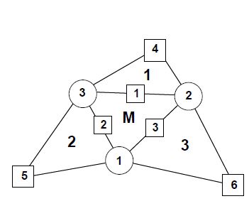
|
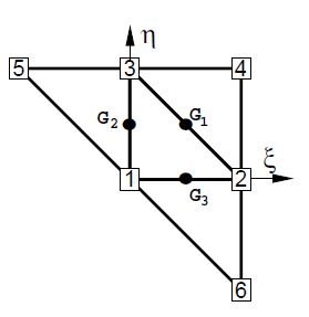
|
| (a) | (b) |
| Figure 1: (a) Patch of three node triangular elements including the central triangle (M) and three adjacent triangles (1, 2 and 3); (b) Patch of elements in the isoparametric space | |
3.1 Definition of the Element Geometry and Computation of Membrane Strains
A quadratic approximation of the geometry of the four elements patch is chosen using the position of the six nodes in the patch. It is useful to define the patch in the isoparametric space using the nodal positions given in the Table 1 (see also Fig.1).
| 1 | 2 | 3 | 4 | 5 | 6 | |
| 0 | 1 | 0 | 1 | -1 | 1 | |
| 0 | 0 | 1 | 1 | 1 | -1 |
The quadratic interpolation is defined by
|
|
(29) |
with ()
|
|
(30) |
This interpolation allows to computing the displacement gradients at selected points in order to use an assumed strain approach. The computation of the gradients is performed at the mid side points of the central element of the patch denoted by , and in Fig. 1. This choice has the following advantages.
- Gradients at the three mid side points depend only on the nodes belonging to the two elements adjacent to each side. This can be easily verified by sampling the derivatives of the shape functions at each mid-side point.
- When gradients are computed at the common mid-side point of two adjacent elements, the same values are obtained, as the coordinates of the same four points are used. This in practice means that the gradients at the mid-side points are independent of the element where they are computed. A side-oriented implementation of the finite element will therefore lead to a unique evaluation of the gradients per side.
The Cartesian derivatives of the shape functions are computed at the original configuration by the standard expression
|
|
(31) |
where the Jacobian matrix at the original configuration is
|
|
(32) |
The deformation gradients on the middle surface, associated to an arbitrary spatial Cartesian system and to the material cartesian system defined on the middle surface are related by
|
|
(33) |
The membrane strains within the central triangle are obtained using a linear assumed strain field , i.e.
|
|
(34) |
with
|
|
(35) |
where are the membrane strains computed at the three mid side points ( see Fig.1). In Eq.(35) , etc.
The gradient at each mid side point is computed from the quadratic interpolation (29):
|
|
(36) |
Substituting Eq.(11) into (35) and using Eq.(9) gives the membrane strain vector as
|
|
(37) |
and the virtual membrane strains as
|
|
(38) |
We note that the gradient at each mid side point depends only on the coordinates of the three nodes of the central triangle and on those of an additional node in the patch, associated to the side where the gradient is computed.
Combining Eqs.(38), (36) and (29) gives
|
|
(39.a) |
with
|
|
(39.b) |
where is the patch displacement vector, contains the three virtual displacement of node and is the membrane strain matrix. An explicit form of is given in [21,22].
Note that the membrane strains within the EBST element are a function of the displacements of the six patch nodes.
3.2 Computation of Curvatures
We will assume the following constant curvature field within each element
|
|
(40) |
where is the assumed constant curvature field defined by
|
|
(41) |
where is the area (in the original configuration) of the central element in the patch.
Substituting Eq.(41) into (40) and integrating by parts the area integral gives the curvature vector within the element in terms of the following line integral
|
|
(42) |
where are the components (in the local system) of the normals to the element sides in the initial configuration . The integration by parts of Eq.(41) is typical in finite volume methods for computing second derivatives over volumes by line integrals of gradient terms [16,17,19,21,22]. For the definition of the normal vector , the linear interpolation over the central element is used. In this case the tangent plane components are
|
|
(43.a) |
|
|
(43.b) |
From these expressions it is also possible to compute in the original configuration the element area , the outer normals at each side and the side lengths . Equation (43.b) also allows to evaluate the thickness ratio in the deformed configuration and the actual normal .
The numerical evaluation of the line integral in Eq.(42) results in a sum over the integration points at the element boundary which are, in fact, the same points used for evaluating the gradients when computing the membrane strains. As one integration point is used over each side, it is not necessary to distinguish between sides () and integration points (). In this way the curvatures can be computed by
|
|
(44) |
Eq.(44) is now expressed in terms of the shape functions of the 3-noded triangle (which coincide with the area coordinates [23]). Noting the property of the area coordinates
|
|
(45) |
the expression for the curvature can be expressed as
|
|
(46) |
The gradient is evaluated at each side from the quadratic interpolation
|
|
(47) |
This is a basic difference with respect of the computation of the curvature field in the original Basic Shell Triangle (BST) where the gradient at the side mid-point is computed as the average value between the values at two adjacent elements [17,19,21,22].
Note again than at each side the gradients depend only on the positions of the three nodes of the central triangle and of an extra node (), associated precisely to the side () where the gradient is computed.
Direction t in Eq.(46) can be seen as a reference direction. If a different direction than that given by Eq.(43.b) is chosen at an angle with the former, this has an influence of order in the projection. This justifies Eq.(43.b) for the definition of t as a function exclusively of the three nodes of the central triangle, instead of using the 6-node isoparametric interpolation.
The variation of the curvatures can be expressed as
|
|
(48) |
In Eq.(48)
|
|
(49) |
Details of the derivation of the curvature matrix are given in [21,22,26].
3.3 The EBST1 Element
A simplified and yet very effective version of the EBST element can be obtained by using one point quadrature for the computation of all the element integrals. This element is termed EBST1. Note that this only affects the membrane stiffness matrices and it is equivalent to using a assumed constant membrane strain field defined by an average of the metric tensors computed at each side [21,22].
Numerical experiments have shown that both the EBST and the EBST1 elements are free of spurious energy modes [21,22].
3.4 Boundary Conditions
Elements at the domain boundary, where an adjacent element does not exist, deserve a special attention. The treatment of essential boundary conditions associated to translational constraints is straightforward, as they are the natural degrees of freedom of the element. The conditions associated to the normal vector are crucial in the bending formulation. For clamped sides or symmetry planes, the normal vector must be kept fixed (clamped case), or constrained to move in the plane of symmetry (symmetry case). The former case can be seen as a special case of the latter, so we will consider symmetry planes only. This restriction can be imposed through the definition of the tangent plane at the boundary, including the normal to the plane of symmetry that does not change during the process.
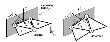
|
|
| Figure 2: Local Cartesian system for the treatment of symmetry boundary conditions |
The tangent plane at the boundary (mid-side point) is expressed in terms of two orthogonal unit vectors referred to a local-to-the-boundary Cartesian system (see Fig.2) defined as
|
|
(50) |
where vector is fixed during the process while direction emerges from the intersection of the symmetry plane with the plane defined by the central element (). The plane (gradient) defined by the central element in the selected original convective Cartesian system () is
|
|
(51) |
the intersection line (side ) of this plane with the plane of symmetry can be written in terms of the position of the nodes that define the side ( and ) and the original length of the side , i.e.
|
|
(52) |
That together with the outer normal to the side (resolved in the selected original convective Cartesian system) leads to
|
|
(53) |
where, noting that is the determinant of the gradient, the normal component of the gradient can be approximated by
|
|
(54) |
For a simple supported (hinged) side, the problem is not completely defined. The simplest choice is to neglect the contribution to the side rotations from the adjacent element missing in the patch in the evaluation of the curvatures via Eq.(42) [17,19,21,22]. This is equivalent to assume that the gradient at the side is equal to the gradient in the central element, i.e.
|
|
(55) |
More precise changes can be however introduced to account for the different natural boundary conditions. One may assume that the curvature normal to the side is zero, and consider a contribution of the missing side to introduce this constraint. As the change of curvature parallel to the side is also zero along the hinged side, this obviously leads to zero curvatures in both directions.
We note finally that for the membrane formulation of the EBST element, the gradient at the mid-side point of the boundary is assumed equal to the gradient of the main triangle.
More details on the specification of the boundary conditions on the EBST element can be found in [21,22].
3.5 Explicit Solution Scheme
For simulations presenting large geometrical and/or material non-linearities, involving frictional contact conditions on complex geometries, convergence is difficult to achieve with implicit schemes. In these cases an explicit solution algorithm is typically most advantageous. The explicit scheme provides the solution for dynamic problems and also for quasi-static problems if an adequate damping is chosen.
The dynamic equations of motion to solve are of the form
|
|
(56) |
where is the nodal displacement vector for the whole mesh, is the mass matrix, is the damping matrix and the dot means the time derivative. The solution is performed using the central difference method. To make the method competitive a diagonal (lumped) matrix is typically used and is taken proportional to . As usual, mass lumping is performed by assigning one third of the triangular element mass to each node in the central element.
The explicit solution scheme can be summarized as follows. At each time step where the displacements u have been computed:
- Compute the residual forces . This follows the steps described in Box 1.
- Compute the accelerations at time
(57) - Compute the velocities at time
(58) - Compute the displacements at time
(59) - Update the shell geometry
- Check frictional contact conditions
where is the diagonal (lumped) mass matrix.
|
Generate the actual configuration Compute the metric tensor and the curvatures . Then at each layer compute the (approximate) right Cauchy-Green tensor. From (14)
Compute the total (21) and elastic (22) deformations at each layer
Compute the trial Hencky elastic stresses (23) at each layer
Check the plasticity condition and return to the plasticity surface. If necessary correct the plastic strains at each layer Compute the second Piola-Kirchhoff stress vector and the generalized stresses
Where is the weight of the through-the-thickness integration point and is the number of layers (integration points) across the thickness. Recall that is the current distance of the layer to the mid-surface and not the original distance. However, for small strain plasticity this distinction is not important. This computation of stresses is exact for an elastic problem. Compute the residual force vector for each element from
| ||||||||||||||||
The formulation of the EBST element described above has been implemented in the explicit dynamic code STAMPACK [31]. This code has been used for the structural analysis computations shown in the examples section.
For further details see [21,22].
4 Aeroelastic Analysis
Wind loading analysis is mandatory in outdoor membrane structures such as inflatable structures formed by low pressure inflatable tubes. Aeroelastic forces can induce the instability and failure of the structure. The accurate computation of wind forces is also essential for the correct design of the anchoring system. A simple weakly coupled staggered aeroelastic scheme has been implemented for the EBST rotation-free shell triangle described in the previous sections. The computation of the wind forces on the membrane structure is performed at each time step using the Tdyn fluid-dynamic code based on the solution of the Navier-Stokes equations for a viscous flow using a stabilized finite element formulation [33]. Wind forces are used to compute the membrane deformations via the EBST element. This naturally introduces changes in the geometry of the domain where the aerodynamic analysis is performed. These changes are taken into account in the fluid-dynamic analysis at the next time step and so on. The transfer of data between the aerodynamic and structural analysis codes is performed via “ad-hoc” interface for data interchange in fluid-structure interaction problems [27, 28, 32].
5 Examples
All units in the examples are given in the international unit system.
5.1 Inflation of a Sphere
As the EBST element uses a quadratic interpolation of geometry, the existance of membrane locking must be assessed. For this example an originally curved surface is considered, where a standard linear strain triangle would lead to membrane locking. The example is the inflation of a spherical shell under internal pressure. An incompressible Mooney-Rivlin constitutive material have been considered [21, 22]. The three meshes of EBST elements considered to evaluate convergence are shown in Fig. 3.a-c. The value of the actual radius as a function of the internal pressure is plotted in Fig. 3.d for the different meshes and is also compared with the analytical solution. It can be seen that with a few degrees of freedom it is possible to obtain an excellent agreement for the range of strains considered. The final value corresponds to a thickness radius ratio of . No membrane locking has therefore been detected in this problem. For more details see [21, 22, 29].
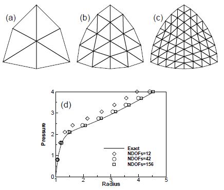
|
| Figure 3: Inflation of sphere of Mooney-Rivlin material. (a)-(c) EBST meshes used in the analysis (d)Radius as a function of the internal pressure |
5.2 Inflation of a Square Airbag Against a Spherical Object
The next example is the inflation of a square airbag supporting a spherical object. The lower surface part of the airbag is limited by a rigid plane and on the upper part a spherical dummy object is set to study the interaction between the airbag and the object. The material properties are given in [21, 22, 30].
The airbag geometry is initially square with an undeformed side length of . Only one quarter of the geometry has been modelled due to symmetry. The thickness considered is and the inflation pressure is . Using a density , pressure is linearly increased from 0 to the final value in . The spherical object has a radius and a mass of (one quarter), and is subjected to gravity load during all the process.
The mesh has 8192 EBST elements and 4225 nodes on the surface of the airbag. Figure 4 shows the deformed configurations for three different times. The sequence on the left figure corresponds to an analysis including full bending effects and the sequence on the right is the result of a pure membrane analysis. Note that the membrane solution presents artificial (numerical) wrinkles which dissappear when using the full bending formulation presented in this paper.
5.3 Inflation/Deflation of a Closed Tube
This problem studies the inflating and de-inflating of a tube with a semi-spherical end cap. The tube diameter is , its total length is and the thickness . The material has the following properties , , . The tube is inflated fast until a pressure of and when pressure is released the tube de-inflates and falls under self weight. The analysis is performed with a mesh of 16704 EBST elements and 8501 nodes modelling a quarter of the geometry. A rigid frictionless base is assumed. Self contact is also included to avoid penetrations. The evolution of the tube walls during the de-inflating process are shown in Fig. 5. For this very thin shell, the differences between a full bending solution and a pure membrane solution are less marked.
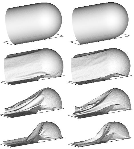
|
| Figure 5: Inflation and deflation of a closed tube. , , . Left figure: results obtained with the full bending formulation. Right figure: results obtained with a pure membrane solution |
5.4 Inflation of a Tubular Arch
The next example is the analysis of a tubular arch. This kind of archs are joined together to form large inflatable structures for a wide range of applications as shown in the following examples. The tubular arch has a internal diameter of ; is total length is and the heigth is . The tube thickness is , the constitutive material is polyamid with Young modulus and Poisson ratio . Due to geometric symmetrys one quarter of the tube was discretized with 33600 triangular elements (17061 nodes). The simulation includes two stages. First the tube is left fall down under gravity action. Second an internal pressure of is applied in a short time and kept constant afterwards until the full inflation of the tube is reached.
Figure 6 shows deformed configurations for different instants of the process.
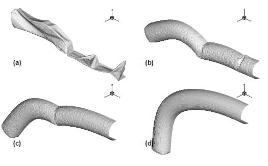
|
| Figure 6: Inflation of a tubular arch. (a) Deflated tube. (b),(c) Deformed configurations during the inflation process. (d) Final inflated configuration |
5.5 Impact of Rigid Spheres on an Inflated Pavilion
Figure 7 shows the impact of two rigid spheres on an inflatable structure ressembling a mushroom. The surface has been discretized with a relative coarse mesh of EBST elements. This example simulates the effect of children jumping or walking on an inflatable structure. Frictional contact conditions and elastic material properties are assumed. The pavilion structure is inflated to a low pressure. The sphere on the top of the pavilion is linked to the structure. The bouncing sphere was shot to the structure. The results observed agree very well with the expected behaviour.
A numerical experiment was performed next for reproducing the inflating and deflating process of the mushroom shape pavilion. Figure 8 represents the inflating process.
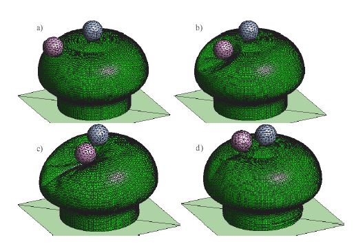
|
| Figure 7: Impact of two spheres on a inflatable structure. Deformed shape at different times |
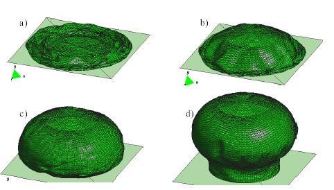
|
| Figure 8: Inflation of a membrane structure. Geometry at different times during the inflating process |
5.6 Deployment of a Spinnaker Sail
Figure 9 shows the simulation of the deployment of a spinnaker sail under the wind action. An elastic material (Naylon) is used with a coarse mesh of 730 EBST elements. The material properties used are , , . The wind pressure force is obtained using the Tdyn CFD code [33]. The apparent wind velocity used is 4. The sail deployment process agrees very well to the real behaviour. The objective was to determine the stress level on the sail.
5.7 Examples of Practical Constructions of Membrane Structures with Low Pressure Inflatable Tubes
Figure Figure 10 presents a pavilion of 150 m for a telecommunication company in Spain. The pavilion is made by assembling some 70 low pressure tubes like the one showed in Figure Figure 6. The tubes are joined together to create the pavilion space. The complexity of the shape required extensive aerodynamic analysis to guarantee the stability of the structure. This pavilion visited some 15 cities in Spain during 2005.
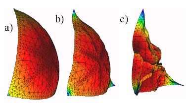
| |
| Figure 9: Spinnaker sail. Sequence of deployment | |
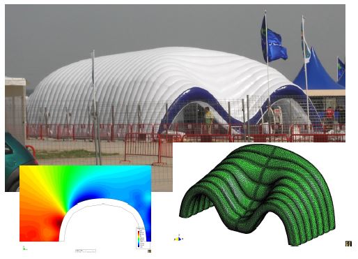
|
| Figure 10: Inflated pavilion for a telecommunication exhibition built by assembly of low pressure inflatable tubes. Triangular mesh on the pavilion surface and results of the aerodynamic analysis |

| |
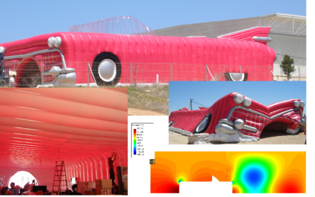
| |
| Figure 11: Cadillac style exhibition pavilion built by assembly of low pressure analysis tubes. Geometry and results of the aerodynamic analysis | |
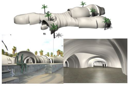
|
| Figure 12: Exhibition hall in Barcelona built by assembly of low pressure inflatable tubes. Images of the design project |
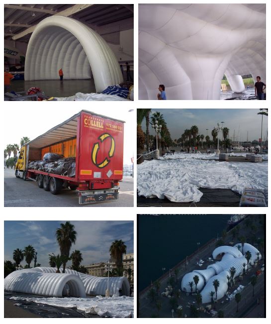
|
| Figure 13: Inflatable exhibition hall in Barcelona harbour. Images of the construction of the different modules, transport, lay-out and inflating operations |
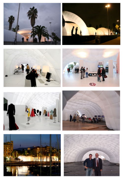
|
| Figure 14: Inflatable exhibition hall in Barcelona harbour. Images of outside and inside spaces. Lower frame shows the first and third authors of the paper (from right to left) |
Figure 11 shows an inflated pavilion of some 200 m simulating and old cadillac automotive for and itinerant exhibition in Spain (2005). The flat geometry of the ceiling was a challenge for the designers. Extensive structural and aerodynamic analysis were performed using the Tdyn code [33] to guarantee the integrity of the structure.
Figure 12 shows the design shape of a relative large inflatable exhibition hall (1600m) built in the harbour area of the city of Barcelona on December 2004. Figure 13 shows some stages of the construction of the different inflatable modules of the pavilion and images of the transport, lay-out and inflating operations. Note the simplicity of the transport logistics, compared with the dimensions of the structure, involving a few bags easily carried in a mid-size vehicle. Figure 14 shows images of the outside and inside spaces of the pavilion containing a display of innovative concepts and products in modern art, fashion and information technologies.
Figure 15 shows images of a mid-size inflatable pavilion (250m) built for an itinerant exhibition on Gaudi. The exhibition visited some 20 cities in Spain in 2002. Some images of the outside and inside of the pavilion are shown in Fig 16. More details are given in [25].
Figure 17 shows images of an inflatable pavilion of formed by assembling of 6 cylindrical halls. The pavilion was built in an old train station in Barcelona in December 2004 for an exhibition on the history of Civil Engineering in Catalonia. Some views of the pavilion entrance and the inside are shown in Fig.18. For more details of this inflatable pavilion see [25].
Figures 19 and 20 finally show images of designs of innovative inflatable pavilions and halls formed by low pressure inflatable tubes. The versatility of the tube assembly process allows the design and construction of quite complex shapes of artistic and architectural value in a simple and economical manner.
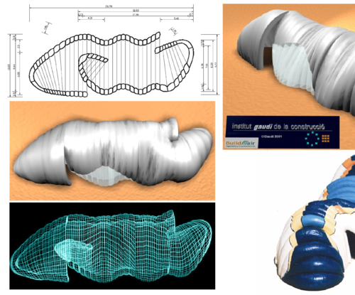
| |
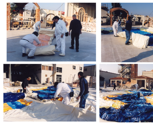
| |
| Figure 15: Pavilion for an itinerant Gaudi Exhibition in Spain. Geometry and lay-out of the inflation process | |
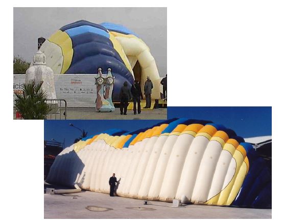
| |
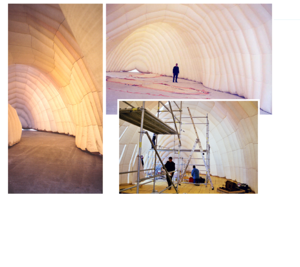
| |
| Figure 16: Inflatable pavilion for Gaudi Exhibition. Images of outside and inside spaces | |
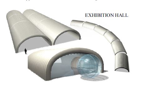
| |
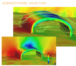
|
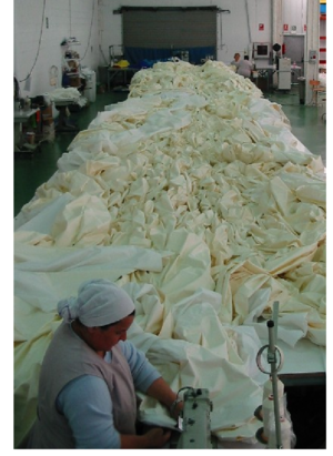
|
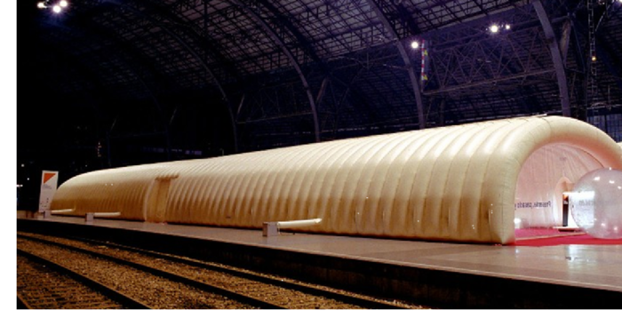
| |
| Figure 17: Inflatable exhibition hall in Barcelona. Original design. Results of the aerodynamic analysis. Sewing of membrane patterns and final construction | |
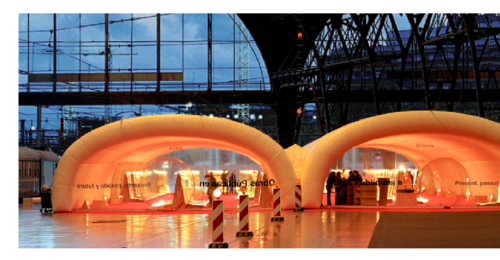
| |
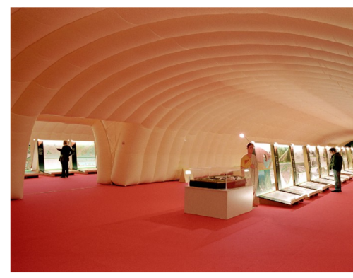
| |
| Figure 18: Images of inflatable exhibition hall in Barcelona | |
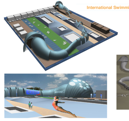
| |
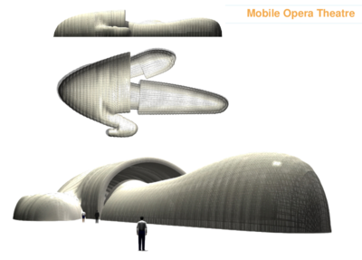
| |
| Figure 19: Projects of low pressure inflatable pavilions. Above: pavilion for an international swimming competition. Below: mobile opera theatre | |
6 Concluding Remarks
We have presented in the paper the formulation of a rotation-free enhanced basic shell triangle (EBST) for analysis of thin membranes and inflatable structures. The element is based on an assumed constant curvature field expressed in terms of the nodal deflections of a patch of four elements and an assumed linear membrane strain field for the in-plane behaviour. A simple and economic version of the element using a single integration point has been presented. The element has proven to be an excellent candidate for solving practical problems in the design and analysis of low pressure inflatable structures under different loading conditions as demonstrated in the examples of application shown.
A large variety of membrane structures built by assembly of low pressure inflatable tubes has been presented showing the versalitiy and potential of this type of constructions in practice.
Acknowledgments
The second author is a member of the scientific staff of the Science Research Council of Argentina (CONICET). The financial support of CIMNE, CONICET and Agencia Córdoba Ciencia S.E. and the support of the companies QUANTECH ATZ SA (http://www.quantech.es/) and COMPASS Ingeniería y Sistemas SA (http://www.compassis.com/) providing the codes STAMPACK [31] and Tdyn [33] are gratefully acknowledged. Thanks are also given to BuildAir Ingeniería y Arquitectura SA (http://www.buildair.com/) for providing photographs of practical constructions of inflatable structures.
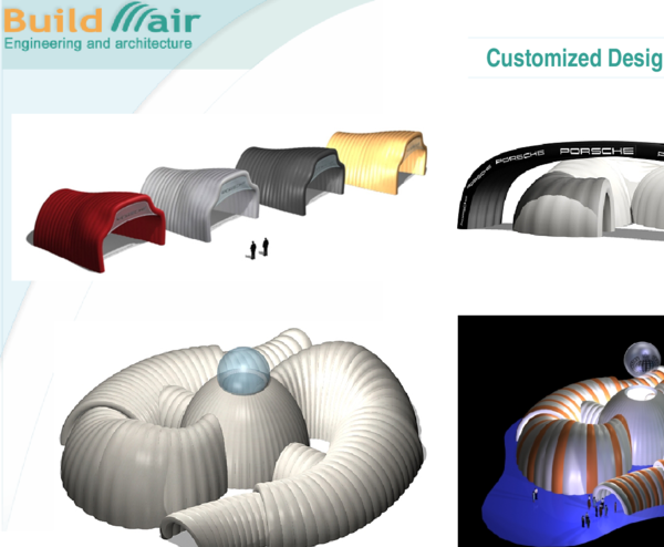
|
| Figure 20: Projects of pavilions formed by low pressure inflatable tubes |
References
[1] Inflatable structures for engineering and architecture applications. BuildAir Ingeniería y Arquitectura SA, www.buildair.com, 2007
[2] Plant RH, Liapis S, Telionis DP (1996) Flood Protection using Inflatable Dams. Natural Disaster Reduction Conference. Washington December 3-5:264-265
[3] Rehmet M, Bauder C, Schäfer, I Kröplin BH (1994) Solar Powered Airship Project. International Conference Remotely Piloted Vehicles, Bristol
[4] Beukers A, Molder OV, Vermeeren CAJR (2001) Inflatable Structures in Space Engineering. Journal of the IASS
[5] ILC Dover, World leader in innovative flexible solutions (2000). http://www.ilcdover.com
[6] New Methodologies for Design and Manufacturing of Inflated Structures (INFLAST) (Brite-Euram Contract NAº BRPR-CT97-0448). Consortium: CIMNE: BAZAN, S.A., CASA, S.A., NOVURANIA, S.p.A., IRD a/s, Universitat Stutt-gart, Airship Technologies, GmbH. Project finished on May 2000
[7] Sadeh WZ, Criswell ME A generic inflatable structure for a lunar/martian base. Proceeding of the Ebgineering, Construction and Operations in Space IV 1146-1156
[8] Nowak PS, Sadeh WZ, Morroni LA (1992), Geometric modeling of inflatable structures for lunar base. Journal of Aerospace Engineering 5(3):311-322
[9] Oñate E, Kröplin B (Eds.) (2003) Proceedings of the 1st. International Conference on Textile Composites and Inflatable Structures I, CIMNE, Barcelona
[10] Oñate E, Kröplin B (Eds.) (2005) Textile Composites and Inflatable Structures I, Springer, Netherlands
[11] Oñate E, Kröplin B (Eds.) (2005) Proceedings of the 2nd. International Conference on Textile Composites and Inflatable Structures II, CIMNE, Barcelona
[12] Taylor RL (2001) Finite element analysis of membrane structures. Publication 203, CIMNE, Barcelona
[13] Oñate E (1994) A review of some finite element families for thick and thin plate and shell analysis. Publication 53, CIMNE, Barcelona
[14] Hampshire JK, Topping BHV, Chan HC (1992) Three node triangular elements with one degree of freedom per node. Engng. Comput. 9:49–62,
[15] Phaal R, Calladine CR (1992) A simple class of finite elements for plate and shell problems. II: An element for thin shells with only translational degrees of freedom. Int. J. Num. Meth. Engng. 35:979–996
[16] Oñate E, Cervera M (1993) Derivation of thin plate bending elements with one degree of freedom per node. Engineering Computations 10:553–561
[17] Oñate E, Zárate F (2000) Rotation-free plate and shell triangles. Num. Meth. Engng. 47:557–603
[18] Cirak F, Ortiz M (2000) Subdivision surfaces: A new paradigm for thin-shell finite element analysis. Int. J Num. Meths. Engng. 47:2039–2072
[19] Flores FG, Oñate E (2001) A basic thin shell triangle with only translational DOFs for large strain plasticity. Int. J. Num. Meths. Engng. 51:57–83.
[20] Cirak F, Ortiz M (2001) Fully -conforming subdivision elements for finite deformations thin-shell analysis. Num. Meths. Engng. 51:813–833
[21] Flores FG, Oñate E (2005) Improvements in the membrane behaviour of the three node rotation-free BST shell triangle using an assumed strain approach. Comput. Meth. Appl. Mech. Engng. 194(6–8):907–932
[22] Oñate E, Flores FG (2005) Advances in the formulation of the rotation-free basic shell triangle. Comput. Meth. Appl. Mech. Engng. 194(21-24):2406-2443
[23] Zienkiewicz OC, Taylor RL (2005) The finite element method. Vol II: Solid Mechanics, Oxford, Elsevier
[24] Ogden RW (1972) Large deformation isotropic elasticity: on the correlation of theory and experiments for incompressible rubberlike solids. Proc. Royal Society London A. 326:565–584
[25] Marcipar J, Oñate E, Miquel J (2005) Experiences in the design analysis and construction of low pressure inflatable structures. Textile Composites and Inflatable Structures I, E. Oñate and B. Kröplin (Eds.), Springer
[26] Flores F, Oñate E (2005) Applications of a rotation-free triangular element for finite strain analysis of thin shells and membranes. Textile Composites and Inflatable Structures I, E. Oñate and B. Kröplin (Eds.), Springer
[27] Pons J, Oñate E, Flores F, García J, Ribó R, Marcipar J (2005) Numerical and experimental values comparison for an inflatable structure. Textile Composites and Inflatable Structures II, E. Oñate and B. Kröplin (Eds.), CIMNE, Barcelona
[28] GiD. The personal pre/postprocessor (2007), CIMNE, Barcelona,
www.gidhome.com
[29] Needleman A (1977) Inflation of spherical rubber ballons. Solids and Structures 13:409–421
[30] Marklund PO, Nilsson L (2002) Simulation of airbag inflation processes using a coupled fluid structure approach. Computational Mechanics 29:289–297
[31] STAMPACK (2007) An explicit dynamic code for sheet stamping analysis. Quantech ATZ SA (www.quantech.es)
[32] A communication library for fluid-structure interaction analysis (2007). Compass Ingeniería y Sistemas SA, www.compassis.com
[33] Tdyn (2007) Finite element code for fluid dynamics and thermal analysis. Compass Ingeniería y Sistemas SA, www.compassis.com
Document information
Published on 01/01/2007
Licence: CC BY-NC-SA license
Share this document
Keywords
claim authorship
Are you one of the authors of this document?
