m (Cinmemj moved page Draft Samper 307425316 to Casas et al 2019a) |
|||
| (28 intermediate revisions by the same user not shown) | |||
| Line 516: | Line 516: | ||
[[File:Draft_Samper_307425316_7710_scales_DEM.png|510px|Number of particles associated to cubic domains for a fixed proportion of volume occupied by the particles (1x10<sup>-1</sup>) as a function of the equivalent side length of the domain. The curves corresponding to different numbers of particles are included, as well as the upper limit sizes for clay, silt and sand, as representative granular materials. The scattered points correspond to different industrial application examples: coal, salt and nuts pneumatic conveying (volume per linear meter for typical pipe diameters); fluidized bed experiments of <span id='citeF-143'></span>[[#cite-143|[143]]], showing the different Geldart categories; and catalytic cracking (FCC) for the production of gasoline.]] | [[File:Draft_Samper_307425316_7710_scales_DEM.png|510px|Number of particles associated to cubic domains for a fixed proportion of volume occupied by the particles (1x10<sup>-1</sup>) as a function of the equivalent side length of the domain. The curves corresponding to different numbers of particles are included, as well as the upper limit sizes for clay, silt and sand, as representative granular materials. The scattered points correspond to different industrial application examples: coal, salt and nuts pneumatic conveying (volume per linear meter for typical pipe diameters); fluidized bed experiments of <span id='citeF-143'></span>[[#cite-143|[143]]], showing the different Geldart categories; and catalytic cracking (FCC) for the production of gasoline.]] | ||
|- style="text-align: center; font-size: 75%;" | |- style="text-align: center; font-size: 75%;" | ||
| − | | colspan="1" | '''Figure 1:''' Number of particles associated to cubic domains for a fixed proportion of volume occupied by the particles (1x10<sup>-1</sup>) as a function of the equivalent side length of the domain. The curves corresponding to different numbers of particles are included, as well as the upper limit sizes for clay, silt and sand, as representative granular materials. The scattered points correspond to different industrial application examples: coal, salt and nuts pneumatic conveying (volume per linear meter for typical pipe diameters); fluidized bed experiments of <span id='citeF-143'></span>[[#cite-143|[143]]], showing the different Geldart categories; and catalytic cracking (FCC) for the production of gasoline. | + | | colspan="1" | '''Figure 1:''' Number of particles associated to cubic domains for a fixed proportion of volume occupied by the particles (1x10<sup>-1</sup>) as a function of the equivalent side length of the domain. The curves corresponding to different numbers of particles are included, as well as the upper limit sizes for clay, silt and sand, as representative granular materials. The scattered points correspond to different industrial application examples: coal, salt and nuts pneumatic conveying (volume per linear meter for typical pipe diameters); fluidized bed experiments of Geldart <span id='citeF-143'></span>[[#cite-143|[143]]], showing the different Geldart categories; and catalytic cracking (FCC) for the production of gasoline. |
|} | |} | ||
| Line 558: | Line 558: | ||
<li>To study the range of applicability of the Maxey–Riley equation as a model for the motion of the individual particles submerged in a fluid, improving the current knowledge on the subject and generating, where possible, practical estimates of direct application to numerical modelling. </li> | <li>To study the range of applicability of the Maxey–Riley equation as a model for the motion of the individual particles submerged in a fluid, improving the current knowledge on the subject and generating, where possible, practical estimates of direct application to numerical modelling. </li> | ||
<li>To study current alternatives for the numerical treatment of the history term in the equation of motion and compare them. </li> | <li>To study current alternatives for the numerical treatment of the history term in the equation of motion and compare them. </li> | ||
| − | <li>To improve on the method of quadrature (the history term involves a time integral, as will be explained later) proposed by <span id='citeF-353'></span>[[#cite-353|[353]]] and provide a detailed study of its efficiency and accuracy, providing convincing evidence that it is not necessary to neglect this term to have an efficient numerical method. </li> | + | <li>To improve on the method of quadrature (the history term involves a time integral, as will be explained later) proposed by van Hinsberg <span id='citeF-353'></span>[[#cite-353|[353]]] and provide a detailed study of its efficiency and accuracy, providing convincing evidence that it is not necessary to neglect this term to have an efficient numerical method. </li> |
<li>To report an account of relevant application examples of the proposed strategy with interest to the industry, as well as of the different technologies developed for their particular requirements. </li> | <li>To report an account of relevant application examples of the proposed strategy with interest to the industry, as well as of the different technologies developed for their particular requirements. </li> | ||
<li>To generalize a stabilized finite element method and use it to discretize the backward-coupled flow equations. </li> | <li>To generalize a stabilized finite element method and use it to discretize the backward-coupled flow equations. </li> | ||
| Line 587: | Line 587: | ||
==1.3 Outline of this document== | ==1.3 Outline of this document== | ||
| − | The core of this work is contained in Chapters | + | The core of this work is contained in Chapters [[#2 The Maxey–Riley equation|2]] to [[#4 Forward and backward-coupled particulate flows|4]]. Of these, Chapter [[#2 The Maxey–Riley equation|2]] is the most theoretical in character. It is devoted to the analysis of the Maxey–Riley equation, as a fundamental model for the description of the motion of individual particles in a fluid, which at this point is assumed to be described by a known field. Section [[#2.2 Range of validity|2.2]] systematically explores the range of validity of the model with respect to several criteria, first in terms of the nondimensional values that appear in the equation itself and later in terms of additional variables involving a selection of simplifications introduced a priori in the development of the theory. In Section [[#2.3 Scaling analysis|2.3]] we apply a scaling analysis to the different terms in the model, providing estimates of their relative magnitude that may be applied in practice to simplify the basic model by neglecting the less important terms. Section [[#2.4 Summary|2.4]] contains a summary of the main results of the chapter, including Tables [[#table-2|2]], [[#table-4|4]] and [[#table-5|5]], that list the most important numerical estimates. |
| − | Chapter [[#3 The numerical solution of the Maxey–Riley equation|3]] shifts from the analytic point of view of Chapter [[#2 The Maxey–Riley equation|2]] to the study of different numerical techniques to solve the Maxey–Riley equation, providing a detailed description of the algorithms involved. We emphasize the treatment of the history force term, whose numerical solution remains challenging, and that is often ignored for this reason. In Section [[#3.2 Overview of approaches for the treatment of the Boussinesq–Basset term|3.2]] we provide a state of the art concerning the numerical treatment of this term, comparing the accuracies of several methods of quadrature. Section [[#3.3 Improvements on the MAE|3.3]] contains the description of our method of choice for the quadrature, proposed by <span id='citeF-353'></span>[[#cite-353|[353]]], and of the extensions and improvements we have developed based on it. Section [[#3.4 Overall algorithm|3.4]] contains the description of the overall algorithm for the time integration of the equation of motion including the history term. In Section [[#3.5 The fractional calculus perspective|3.5]] we make a stop to connect the general theory of fractional calculus to the Maxey–Riley equation, which had only been very superficially sketched before. This section appears at this point to take advantage of the terminology and concepts introduced in the previous developments. Section [[#3.6 Performance of the methodology|3.6]] is devoted to a systematic analysis of the accuracy and efficiency of the numerical method of solution, applying it to a sequence of benchmarks of increasing complexity. We close the chapter with a summary of the most important results and developments. | + | Chapter [[#3 The numerical solution of the Maxey–Riley equation|3]] shifts from the analytic point of view of Chapter [[#2 The Maxey–Riley equation|2]] to the study of different numerical techniques to solve the Maxey–Riley equation, providing a detailed description of the algorithms involved. We emphasize the treatment of the history force term, whose numerical solution remains challenging, and that is often ignored for this reason. In Section [[#3.2 Overview of approaches for the treatment of the Boussinesq–Basset term|3.2]] we provide a state of the art concerning the numerical treatment of this term, comparing the accuracies of several methods of quadrature. Section [[#3.3 Improvements on the MAE|3.3]] contains the description of our method of choice for the quadrature, proposed by Hinsberg et al. <span id='citeF-353'></span>[[#cite-353|[353]]], and of the extensions and improvements we have developed based on it. Section [[#3.4 Overall algorithm|3.4]] contains the description of the overall algorithm for the time integration of the equation of motion including the history term. In Section [[#3.5 The fractional calculus perspective|3.5]] we make a stop to connect the general theory of fractional calculus to the Maxey–Riley equation, which had only been very superficially sketched before. This section appears at this point to take advantage of the terminology and concepts introduced in the previous developments. Section [[#3.6 Performance of the methodology|3.6]] is devoted to a systematic analysis of the accuracy and efficiency of the numerical method of solution, applying it to a sequence of benchmarks of increasing complexity. We close the chapter with a summary of the most important results and developments. |
Chapter [[#4 Forward and backward-coupled particulate flows|4]] moves even further toward practice, being eminently applied in nature. We consider a series of applications representative to different families of industrial problems, describing several developments involved in their solution as we go along. Section [[#4.2 Beyond the MRE|4.2]] discusses how the equation of motion considered in the previous chapters can be modified using empirical relations to extend its range of applicability beyond the limits studied in Chapter [[#2 The Maxey–Riley equation|2]], for this will be necessary in the industrial applications that are considered later on. In Section [[#4.3 The continuous-phase problem|4.3]] we introduce the fluid phase as a problem to be solved for the first time, for which we make use of a well-established stabilized finite element formulation. We describe it in sufficient detail to clarify the terminology and set the stage for the generalizations introduced in Section [[#4.3 The continuous-phase problem|4.3]]. In Section [[#4.4 Derivative recovery|4.4]] we discuss the problem of derivative recovery, as a step necessary to obtain accurate estimates of the derivatives of the fluid field, once a solution is produced by the fluid solver. We give a brief state-of-the-art and compare several alternatives compatible to the finite element method. The description of the particles-fluid coupling is described very briefly in Section [[#4.5 Forward coupling|4.5]] where we basically bring together the different algorithmic parts involved. We quickly turn to the first application example, which is the subject of Section [[#4.6 Application example: T-junction bubble trapping|4.6]]. It consists on the numerical simulation of the phenomenon of air bubble trapping in T-shaped pipe junctions, which was only recently first studied by Vigolo et al. <span id='citeF-356'></span>[[#cite-356|[356]]]. This test exemplifies the use of the one-way coupled strategy, with no inter-particle interactions, representative of low-Reynolds number internal flows with low-density suspensions of small particles. We continue on to the study of the next test application in Section [[#4.7 Application example: Particle impact drilling|4.7]], where we study particle impact drilling, a technology used in the oil and gas industries to produce high penetration rate drilling systems. Here we again make use of a one-way coupled strategy for the fluid-particles coupling, although this time we consider the inter-particle contact as well. This is by far the most detailed of the examples provided and corresponds to consultancy work made during the Doctorat Industrial. Before moving on to the final example, the theory related to the backward-coupled flow must be introduced first, based on the theory of multicomponent flows (its rudiments can be found in Appendix [[#13 Multicomponent theory fundamentals|H]]) and the general finite element formulation introduced in Section [[#4.3 The continuous-phase problem|4.3]], which we specialize for this problem. Following this theoretical interlude, we present the last application example, a fluidized bed of Geldard-D particles in Section [[#4.9 Application example: fluidized bed|4.9]]. We close with a summary of the chapter in Section [[#4.10 Summary|4.10]]. | Chapter [[#4 Forward and backward-coupled particulate flows|4]] moves even further toward practice, being eminently applied in nature. We consider a series of applications representative to different families of industrial problems, describing several developments involved in their solution as we go along. Section [[#4.2 Beyond the MRE|4.2]] discusses how the equation of motion considered in the previous chapters can be modified using empirical relations to extend its range of applicability beyond the limits studied in Chapter [[#2 The Maxey–Riley equation|2]], for this will be necessary in the industrial applications that are considered later on. In Section [[#4.3 The continuous-phase problem|4.3]] we introduce the fluid phase as a problem to be solved for the first time, for which we make use of a well-established stabilized finite element formulation. We describe it in sufficient detail to clarify the terminology and set the stage for the generalizations introduced in Section [[#4.3 The continuous-phase problem|4.3]]. In Section [[#4.4 Derivative recovery|4.4]] we discuss the problem of derivative recovery, as a step necessary to obtain accurate estimates of the derivatives of the fluid field, once a solution is produced by the fluid solver. We give a brief state-of-the-art and compare several alternatives compatible to the finite element method. The description of the particles-fluid coupling is described very briefly in Section [[#4.5 Forward coupling|4.5]] where we basically bring together the different algorithmic parts involved. We quickly turn to the first application example, which is the subject of Section [[#4.6 Application example: T-junction bubble trapping|4.6]]. It consists on the numerical simulation of the phenomenon of air bubble trapping in T-shaped pipe junctions, which was only recently first studied by Vigolo et al. <span id='citeF-356'></span>[[#cite-356|[356]]]. This test exemplifies the use of the one-way coupled strategy, with no inter-particle interactions, representative of low-Reynolds number internal flows with low-density suspensions of small particles. We continue on to the study of the next test application in Section [[#4.7 Application example: Particle impact drilling|4.7]], where we study particle impact drilling, a technology used in the oil and gas industries to produce high penetration rate drilling systems. Here we again make use of a one-way coupled strategy for the fluid-particles coupling, although this time we consider the inter-particle contact as well. This is by far the most detailed of the examples provided and corresponds to consultancy work made during the Doctorat Industrial. Before moving on to the final example, the theory related to the backward-coupled flow must be introduced first, based on the theory of multicomponent flows (its rudiments can be found in Appendix [[#13 Multicomponent theory fundamentals|H]]) and the general finite element formulation introduced in Section [[#4.3 The continuous-phase problem|4.3]], which we specialize for this problem. Following this theoretical interlude, we present the last application example, a fluidized bed of Geldard-D particles in Section [[#4.9 Application example: fluidized bed|4.9]]. We close with a summary of the chapter in Section [[#4.10 Summary|4.10]]. | ||
| Line 597: | Line 597: | ||
We provide a series of appendices that carry substantial content. Our intent in doing so has been more to lighten the main text than to expand it with additional content. Perhaps the idea of ''modularity'', associated to the programming principle, has contaminated our writing style, but we hope it helps comprehension. For instance Appendix [[#6 DEM specifics|A]] contains most of the little text devoted to the discrete element method while Appendix [[#13 Multicomponent theory fundamentals|H]] is devoted to the description of the continuum theory related to the backward-fluid flow. The other appendices include formulas and numerical data of interest mainly to the interested reader willing to program the associated algorithms. | We provide a series of appendices that carry substantial content. Our intent in doing so has been more to lighten the main text than to expand it with additional content. Perhaps the idea of ''modularity'', associated to the programming principle, has contaminated our writing style, but we hope it helps comprehension. For instance Appendix [[#6 DEM specifics|A]] contains most of the little text devoted to the discrete element method while Appendix [[#13 Multicomponent theory fundamentals|H]] is devoted to the description of the continuum theory related to the backward-fluid flow. The other appendices include formulas and numerical data of interest mainly to the interested reader willing to program the associated algorithms. | ||
| − | Finally, the Nomenclature section provides a quick guide for the symbols used throughout. Only the symbols that are exclusively used in a single context, close to their definitions, have been left out of the list, to avoid overpopulating it. | + | Finally, the Nomenclature section provides a quick guide for the symbols used throughout. Only the symbols that are exclusively used in a single context, close to their definitions, have been left out of the list, to avoid overpopulating it. |
=2 The Maxey–Riley equation= | =2 The Maxey–Riley equation= | ||
| Line 810: | Line 810: | ||
The well known Stokes solution of the steady, low Reynolds number flow past a sphere (see Eq.~[[#eq-2.31|2.31]]) is obtained by completely neglecting fluid inertia. By applying the no-slip boundary conditions on the particle surface and the far-field velocity conditions at infinity and expanding the stream function in powers of <math display="inline">\mathit{Re}_p</math>, the hydrodynamic force on the particle can be calculated, to leading <math display="inline">\mathit{Re}_p</math> order, yielding the drag force of the MRE without the Faxén terms (this is the problem solved by Stokes in 1851). However, if one wishes to increase the order of this approximation following the same procedure, one soon realizes that there is no way to fulfil the far field boundary conditions in this case, since the higher order contributions to the perturbation caused by the particle do not vanish at infinity. This phenomenon is known as Whitehead's paradox <span id='citeF-248'></span>[[#cite-248|[248]]]. | The well known Stokes solution of the steady, low Reynolds number flow past a sphere (see Eq.~[[#eq-2.31|2.31]]) is obtained by completely neglecting fluid inertia. By applying the no-slip boundary conditions on the particle surface and the far-field velocity conditions at infinity and expanding the stream function in powers of <math display="inline">\mathit{Re}_p</math>, the hydrodynamic force on the particle can be calculated, to leading <math display="inline">\mathit{Re}_p</math> order, yielding the drag force of the MRE without the Faxén terms (this is the problem solved by Stokes in 1851). However, if one wishes to increase the order of this approximation following the same procedure, one soon realizes that there is no way to fulfil the far field boundary conditions in this case, since the higher order contributions to the perturbation caused by the particle do not vanish at infinity. This phenomenon is known as Whitehead's paradox <span id='citeF-248'></span>[[#cite-248|[248]]]. | ||
| − | Its resolution was possible due to ideas from Oseen, who noted that the assumption by which inertial terms are disregarded (under Eq.~[[#eq-2.8|2.8]]) is only valid near the particle, where viscous effects dominate. But, far from the particle (in particular at a distance such that <math display="inline">\mathit{Re}_p = \mathcal{O}(1)</math>, see <span id='citeF-284'></span>[[#cite-284|[284]]]), the approximation breaks down. This implies that there is an inherent inconsistency in requiring that the Stokes solution be valid in an infinite domain, and that it is necessary to consider inertia far from the particle in order to calculate the higher order corrections to the drag force. The final word on the issue was nonetheless given by <span id='citeF-284'></span>[[#cite-284|[284]]], who, using the technique of matched asymptotic expansions, re-derived Oseen's inertial, first-order correction to the steady drag force, corrected a flaw in Oseen's original reasoning and added an additional term to the expansion: | + | Its resolution was possible due to ideas from Oseen, who noted that the assumption by which inertial terms are disregarded (under Eq.~[[#eq-2.8|2.8]]) is only valid near the particle, where viscous effects dominate. But, far from the particle (in particular at a distance such that <math display="inline">\mathit{Re}_p = \mathcal{O}(1)</math>, see <span id='citeF-284'></span>[[#cite-284|[284]]]), the approximation breaks down. This implies that there is an inherent inconsistency in requiring that the Stokes solution be valid in an infinite domain, and that it is necessary to consider inertia far from the particle in order to calculate the higher order corrections to the drag force. The final word on the issue was nonetheless given by Proudman and Pearson <span id='citeF-284'></span>[[#cite-284|[284]]], who, using the technique of matched asymptotic expansions, re-derived Oseen's inertial, first-order correction to the steady drag force, corrected a flaw in Oseen's original reasoning and added an additional term to the expansion: |
<span id="eq-2.11"></span> | <span id="eq-2.11"></span> | ||
| Line 825: | Line 825: | ||
This way, the contribution from the outer region becomes a correction of the steady drag force, whose leading term, given by <math display="inline">3/8 \mathit{Re}_p</math>, could be used to provide the order of magnitude of this correction. | This way, the contribution from the outer region becomes a correction of the steady drag force, whose leading term, given by <math display="inline">3/8 \mathit{Re}_p</math>, could be used to provide the order of magnitude of this correction. | ||
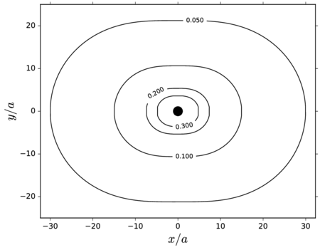
| − | In order to illustrate how it could be used in practice, let us assume that we wish to establish the upper limit to the particle Reynolds number to ensure that the correction is smaller than 5 as a convention to fix the range of validity of the MRE. Then the leading term in Eq.~[[#eq-2.11|2.11]] predicts this to happen for <math display="inline">\mathit{Re}_p \approx 1.4x10^{-1}</math>, and by this point the error in this expression is only <math display="inline">\approx 3x10^{-2}</math>, taking as a reference the empirical drag coefficient by Clift et al. (1978) (which has a root mean square error of <math display="inline">\approx 1x10^{-2}</math> with respect to the empirical data gathered by <span id='citeF-50'></span>[[#cite-50|[50]]] covering the range <math display="inline">0 < \mathit{Re}_p < 4x10^{3}</math>). This means that its range of validity is large enough to estimate the first-effects of inertia for error tolerances lower than 5%. In Fig. [[#img-2|2]] all these different approximations to the drag force are compared. <div id='img-2'></div> | + | In order to illustrate how it could be used in practice, let us assume that we wish to establish the upper limit to the particle Reynolds number to ensure that the correction is smaller than 5 as a convention to fix the range of validity of the MRE. Then the leading term in Eq.~[[#eq-2.11|2.11]] predicts this to happen for <math display="inline">\mathit{Re}_p \approx 1.4x10^{-1}</math>, and by this point the error in this expression is only <math display="inline">\approx 3x10^{-2}</math>, taking as a reference the empirical drag coefficient by Clift et al. (1978) (which has a root mean square error of <math display="inline">\approx 1x10^{-2}</math> with respect to the empirical data gathered by Brown and Lawler <span id='citeF-50'></span>[[#cite-50|[50]]] covering the range <math display="inline">0 < \mathit{Re}_p < 4x10^{3}</math>). This means that its range of validity is large enough to estimate the first-effects of inertia for error tolerances lower than 5%. In Fig. [[#img-2|2]] all these different approximations to the drag force are compared. <div id='img-2'></div> |
{| class="floating_imageSCP" style="text-align: center; border: 1px solid #BBB; margin: 1em auto; width: 100%;max-width: 100%;" | {| class="floating_imageSCP" style="text-align: center; border: 1px solid #BBB; margin: 1em auto; width: 100%;max-width: 100%;" | ||
|- | |- | ||
| Line 1,053: | Line 1,053: | ||
|} | |} | ||
| − | So that the next order correction will be significantly smaller than the classical Faxén correction up to the point when <math display="inline">\mathit{Re}_p</math> is not small any more (in the limit of quasi-steady Stokes flow it holds <math display="inline">\nabla ^4\boldsymbol{u} = 0</math> exactly). This means that in practice the small <math display="inline">\mathit{Re}</math> requirement will guarantee that the Faxén corrections will make a good enough job and thus the restriction Eq.~[[#eq-2.9|2.9]], that is, <math display="inline">a/L\ll 1</math> by itself does not appear to be restrictive, but rather indirectly through the violation of <math display="inline">\mathit{Re}_p \ll 1</math>. A similar argument can be made with the other forces bearing their corresponding Faxén correction. A significant study supporting this conclusion in the context of isotropic turbulence was provided by <span id='citeF-171'></span>[[#cite-171|[171]]], who tested the performance of the Faxén terms for a neutrally buoyant particle in direct numerical simulation (DNS) of isotropic turbulence. Their conclusion was that the first effects of the finite size of the particles were well captured by these terms up to <math display="inline">a \sim 4L</math> (where <math display="inline">L</math> is the Kolmogorov microscale). From then on, inertial (finite <math display="inline">\mathit{Re}_p</math>) effects quickly kick in. | + | So that the next order correction will be significantly smaller than the classical Faxén correction up to the point when <math display="inline">\mathit{Re}_p</math> is not small any more (in the limit of quasi-steady Stokes flow it holds <math display="inline">\nabla ^4\boldsymbol{u} = 0</math> exactly). This means that in practice the small <math display="inline">\mathit{Re}</math> requirement will guarantee that the Faxén corrections will make a good enough job and thus the restriction Eq.~[[#eq-2.9|2.9]], that is, <math display="inline">a/L\ll 1</math> by itself does not appear to be restrictive, but rather indirectly through the violation of <math display="inline">\mathit{Re}_p \ll 1</math>. A similar argument can be made with the other forces bearing their corresponding Faxén correction. A significant study supporting this conclusion in the context of isotropic turbulence was provided by Homann and Bec <span id='citeF-171'></span>[[#cite-171|[171]]], who tested the performance of the Faxén terms for a neutrally buoyant particle in direct numerical simulation (DNS) of isotropic turbulence. Their conclusion was that the first effects of the finite size of the particles were well captured by these terms up to <math display="inline">a \sim 4L</math> (where <math display="inline">L</math> is the Kolmogorov microscale). From then on, inertial (finite <math display="inline">\mathit{Re}_p</math>) effects quickly kick in. |
===2.2.3 Nonsphericity effects=== | ===2.2.3 Nonsphericity effects=== | ||
| Line 1,287: | Line 1,287: | ||
|} | |} | ||
| − | Which, as stated, recover the first order correction due to Oseen for the drag force at <math display="inline">S^* \rightarrow 0</math> (and thus <math display="inline">\alpha _p \rightarrow 0</math>), see Eq.~[[#eq-2.11|2.11]], and also the classic expression by <span id='citeF-49'></span>[[#cite-49|[49]]], at <math display="inline">\mathit{Re}_p \rightarrow 0</math>. | + | Which, as stated, recover the first order correction due to Oseen for the drag force at <math display="inline">S^* \rightarrow 0</math> (and thus <math display="inline">\alpha _p \rightarrow 0</math>), see Eq.~[[#eq-2.11|2.11]], and also the classic expression by Brinkman <span id='citeF-49'></span>[[#cite-49|[49]]], at <math display="inline">\mathit{Re}_p \rightarrow 0</math>. |
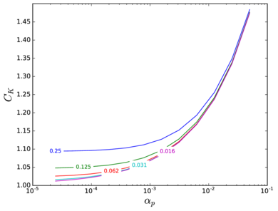
Figure [[#img-5|5]] shows the magnitude of the correction coefficient <math display="inline">C_K</math> for a wide range of solid volume fractions, for different values of <math display="inline">\mathit{Re}_p</math>. Note that the correction to the drag is significant, even for very small Reynolds numbers if the solid volume fraction is greater than 1x10<sup>-3</sup>, in accordance with the rule of thumb of Eq.~[[#eq-2.32|2.32]], and it still appreciable past the 1x10<sup>-4</sup> mark. <div id='img-5'></div> | Figure [[#img-5|5]] shows the magnitude of the correction coefficient <math display="inline">C_K</math> for a wide range of solid volume fractions, for different values of <math display="inline">\mathit{Re}_p</math>. Note that the correction to the drag is significant, even for very small Reynolds numbers if the solid volume fraction is greater than 1x10<sup>-3</sup>, in accordance with the rule of thumb of Eq.~[[#eq-2.32|2.32]], and it still appreciable past the 1x10<sup>-4</sup> mark. <div id='img-5'></div> | ||
| Line 1,331: | Line 1,331: | ||
<span id='citeF-44'></span>[[#cite-44|[44]]] reviewed some of these formulations, recommending the one by Zaichik and Alipchenkov <span id='citeF-381'></span>[[#cite-381|[381]]] as the most comprehensive and robust over a wide range of <math display="inline">\mathit{St}</math> values (see below). | <span id='citeF-44'></span>[[#cite-44|[44]]] reviewed some of these formulations, recommending the one by Zaichik and Alipchenkov <span id='citeF-381'></span>[[#cite-381|[381]]] as the most comprehensive and robust over a wide range of <math display="inline">\mathit{St}</math> values (see below). | ||
| − | Nonetheless, there remain a number of open questions and inconsistencies in the literature that need to be addressed. For instance, there is a significant consensus that the strength of clustering peaks at <math display="inline">\mathit{St} \sim 1</math> <span id='citeF-253'></span><span id='citeF-178'></span>[[#cite-253|[253,178]]], However <span id='citeF-328'></span>[[#cite-328|[328]]] concludes that the level of clustering, measured using a Voronoï tessellation of space, is most strongly related to the Taylor Reynolds number, less so to the average particle volume fraction and negligibly on the Stokes number. Moreover, Uhlmann and Chouippe <span id='citeF-349'></span>[[#cite-349|[349]]] has found that clustering scaling seems to depend on the mode in which it is measured. | + | Nonetheless, there remain a number of open questions and inconsistencies in the literature that need to be addressed. For instance, there is a significant consensus that the strength of clustering peaks at <math display="inline">\mathit{St} \sim 1</math> <span id='citeF-253'></span><span id='citeF-178'></span>[[#cite-253|[253,178]]], However Sumbekova et al. <span id='citeF-328'></span>[[#cite-328|[328]]] concludes that the level of clustering, measured using a Voronoï tessellation of space, is most strongly related to the Taylor Reynolds number, less so to the average particle volume fraction and negligibly on the Stokes number. Moreover, Uhlmann and Chouippe <span id='citeF-349'></span>[[#cite-349|[349]]] has found that clustering scaling seems to depend on the mode in which it is measured. |
Understanding the physical mechanisms that govern the appearance of clustering is of extraordinary importance, not only due to its relevance to the assessment of the validity of the single-particle theory (which includes the MRE), but also in understanding the statistical distribution of particles in space, statistics on the flow properties being sampled (of relevance to the simulation of chemical reactions, for example) and the prediction of the collision rates (of relevance to the study of initiation of rain and snow, for example). Of direct relevance to the present discussion is the study by Aliseda et al. <span id='citeF-4'></span>[[#cite-4|[4]]], where the settling velocity of spheres was measured experimentally in a turbulent channel flow. A notable increase in the settling velocity was observed with respect to quiescent fluid conditions, especially for Stokes numbers on the order of unity. Furthermore, this velocity increased monotonically with the overall volume fraction, indicating the effect of three-way coupling. A phenomenological model based on the idea of particle clusters locally altering the average velocity seen by its constituent particles turned out to explain the observations very well. It is remarkable that the whole study was performed under volume fractions well below the limit given in Eq.~[[#eq-2.32|2.32]], which clearly demonstrates the limitations of the single-particle paradigm. | Understanding the physical mechanisms that govern the appearance of clustering is of extraordinary importance, not only due to its relevance to the assessment of the validity of the single-particle theory (which includes the MRE), but also in understanding the statistical distribution of particles in space, statistics on the flow properties being sampled (of relevance to the simulation of chemical reactions, for example) and the prediction of the collision rates (of relevance to the study of initiation of rain and snow, for example). Of direct relevance to the present discussion is the study by Aliseda et al. <span id='citeF-4'></span>[[#cite-4|[4]]], where the settling velocity of spheres was measured experimentally in a turbulent channel flow. A notable increase in the settling velocity was observed with respect to quiescent fluid conditions, especially for Stokes numbers on the order of unity. Furthermore, this velocity increased monotonically with the overall volume fraction, indicating the effect of three-way coupling. A phenomenological model based on the idea of particle clusters locally altering the average velocity seen by its constituent particles turned out to explain the observations very well. It is remarkable that the whole study was performed under volume fractions well below the limit given in Eq.~[[#eq-2.32|2.32]], which clearly demonstrates the limitations of the single-particle paradigm. | ||
| − | The estimates provided in Section [[#2.2.4.2 Drag modification|2.2.4]] were derived under the assumption of an unbounded array of particles characterized by an average solid fraction under the hypothesis of having a homogeneous suspension. Therefore, the existence of significant inhomogeneities as those caused by preferential concentration in turbulent flows, invalidate the theory and the derived estimates. <span id='citeF-4'></span>[[#cite-4|[4]]] proposed a phenomenological model to explain the effect of preferential concentration in a turbulent suspension of settling particles. They observed that the average settling velocity of the particles belonging to a cluster was reasonably well predicted by Eq.~[[#eq-2.33|2.33]], with | + | The estimates provided in Section [[#2.2.4.2 Drag modification|2.2.4]] were derived under the assumption of an unbounded array of particles characterized by an average solid fraction under the hypothesis of having a homogeneous suspension. Therefore, the existence of significant inhomogeneities as those caused by preferential concentration in turbulent flows, invalidate the theory and the derived estimates. Aliseda et al. <span id='citeF-4'></span>[[#cite-4|[4]]] proposed a phenomenological model to explain the effect of preferential concentration in a turbulent suspension of settling particles. They observed that the average settling velocity of the particles belonging to a cluster was reasonably well predicted by Eq.~[[#eq-2.33|2.33]], with |
<span id="eq-2.39"></span> | <span id="eq-2.39"></span> | ||
| Line 7,221: | Line 7,221: | ||
| compute inter-particle contact (0 or 1) | | compute inter-particle contact (0 or 1) | ||
|- style="border-top: 2px solid;border-bottom: 2px solid;" | |- style="border-top: 2px solid;border-bottom: 2px solid;" | ||
| − | | colspan=' | + | | colspan='3' style="text-align: center;" | Numerical Parameters |
|} | |} | ||
| Line 7,699: | Line 7,699: | ||
The theory of multicomponent media <span id='citeF-109'></span><span id='citeF-179'></span>[[#cite-109|[109,179]]] provides an adequate framework to incorporate both effects into the analysis. This generalization of standard continuum media allows for the presence of an arbitrary number of continuum media superposed over the same spatial region, each with its own set of state variables and constitutive equations though allowing for coupling relations (differential or algebraic equations) to hold. The basic conservation equations are presented in Appendix [[#H Multicomponent theory fundamentals|H]] and can be taken as postulates to start the analysis <span id='citeF-109'></span>[[#cite-109|[109]]]. It is however also possible to derive such equations by applying averaging techniques to the lower-scale description, just as the equations of the continuum can often be derived by applying averaging techniques to the microscopic description of the molecules. | The theory of multicomponent media <span id='citeF-109'></span><span id='citeF-179'></span>[[#cite-109|[109,179]]] provides an adequate framework to incorporate both effects into the analysis. This generalization of standard continuum media allows for the presence of an arbitrary number of continuum media superposed over the same spatial region, each with its own set of state variables and constitutive equations though allowing for coupling relations (differential or algebraic equations) to hold. The basic conservation equations are presented in Appendix [[#H Multicomponent theory fundamentals|H]] and can be taken as postulates to start the analysis <span id='citeF-109'></span>[[#cite-109|[109]]]. It is however also possible to derive such equations by applying averaging techniques to the lower-scale description, just as the equations of the continuum can often be derived by applying averaging techniques to the microscopic description of the molecules. | ||
| − | We present in Appendix [[#H Multicomponent theory fundamentals|H]] a brief description of this averaging process that is a slight generalization of the volume averaging technique of <span id='citeF-8'></span>[[#cite-8|[8]]], see also <span id='citeF-366'></span>[[#cite-366|[366]]]. This averaging process if of interest here as a tool to motivate the numerical method that is later described. We will focus on the fluid-phase averaged equations, since the particle-phase averaged equations are replaced by the DEM in the final algorithm. | + | We present in Appendix [[#H Multicomponent theory fundamentals|H]] a brief description of this averaging process that is a slight generalization of the volume averaging technique of Anderson and Jackson <span id='citeF-8'></span>[[#cite-8|[8]]], see also <span id='citeF-366'></span>[[#cite-366|[366]]]. This averaging process if of interest here as a tool to motivate the numerical method that is later described. We will focus on the fluid-phase averaged equations, since the particle-phase averaged equations are replaced by the DEM in the final algorithm. |
===4.8.1 CFD-DEM model=== | ===4.8.1 CFD-DEM model=== | ||
| Line 8,119: | Line 8,119: | ||
==4.9 Application example: fluidized bed== | ==4.9 Application example: fluidized bed== | ||
| − | In this section we apply the theory presented above to a representative problem in which the backward coupling is unavoidable. This problem was studied numerically recently by <span id='citeF-42'></span>[[#cite-42|[42]]] where the limitations of the volume averaging approach in the CFD-DEM were discussed and highlighted. Our objective here is to see if our finite element-based approach can obtain the same qualitative behaviour obtained with a more conventional approach and to check whether the same problems observed there are reproduced here. | + | In this section we apply the theory presented above to a representative problem in which the backward coupling is unavoidable. This problem was studied numerically recently by Boyce et al. <span id='citeF-42'></span>[[#cite-42|[42]]] where the limitations of the volume averaging approach in the CFD-DEM were discussed and highlighted. Our objective here is to see if our finite element-based approach can obtain the same qualitative behaviour obtained with a more conventional approach and to check whether the same problems observed there are reproduced here. |
| − | The problem at hand is the simulation of a gas-fluidized bed of Geldart-D type <span id='citeF-143'></span>[[#cite-143|[143]]] particles (poppy seeds), that where experimentally studied previously by <span id='citeF-170'></span>[[#cite-170|[170]]]. The container is cylindrical, with a circular base. The geometry corresponds to configurations 2 and 3 in Boyce et al. <span id='citeF-42'></span>[[#cite-42|[42]]], and it is depicted in Fig. [[#img-78a|78a]]. The initial bed size is of 5x10<sup>1</sup> . The most important input parameters are detailed in Table [[#table-15|15]]. In the original work hexahedral cells arranged in a structured way were used for the fluid discretization. We instead employed the sequence of irregular tetrahedral meshes shown in Fig. [[#img-78|78]], were the average sizes (expressed as fractions of the particles' diameter) are calculated as the side of a regular tetrahedron that has the same volume as the average volume of the tetrahedra in the mesh. The average sizes are comparable to the ones used considered in Boyce et al. <span id='citeF-42'></span>[[#cite-42|[42]]]. <div id='img-78a'></div> | + | The problem at hand is the simulation of a gas-fluidized bed of Geldart-D type <span id='citeF-143'></span>[[#cite-143|[143]]] particles (poppy seeds), that where experimentally studied previously by Holland et al. <span id='citeF-170'></span>[[#cite-170|[170]]]. The container is cylindrical, with a circular base. The geometry corresponds to configurations 2 and 3 in Boyce et al. <span id='citeF-42'></span>[[#cite-42|[42]]], and it is depicted in Fig. [[#img-78a|78a]]. The initial bed size is of 5x10<sup>1</sup> . The most important input parameters are detailed in Table [[#table-15|15]]. In the original work hexahedral cells arranged in a structured way were used for the fluid discretization. We instead employed the sequence of irregular tetrahedral meshes shown in Fig. [[#img-78|78]], were the average sizes (expressed as fractions of the particles' diameter) are calculated as the side of a regular tetrahedron that has the same volume as the average volume of the tetrahedra in the mesh. The average sizes are comparable to the ones used considered in Boyce et al. <span id='citeF-42'></span>[[#cite-42|[42]]]. <div id='img-78a'></div> |
<div id='img-78b'></div> | <div id='img-78b'></div> | ||
<div id='img-78c'></div> | <div id='img-78c'></div> | ||
| Line 8,217: | Line 8,217: | ||
|} | |} | ||
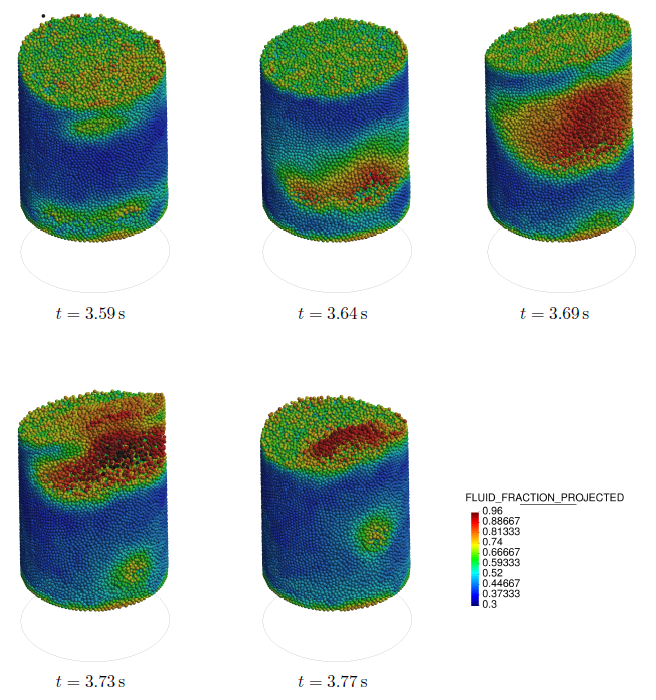
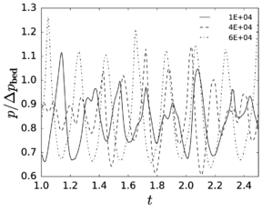
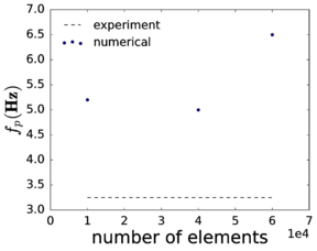
| − | Figure [[#img-78b|78b]] shows a window of the pressure in time as measured at a single point, for the different meshes considered. The pressure values are made dimensionless by dividing them by the average pressure drop in the first 5x10<sup>1</sup> from the bottom of the bed, as measured on the symmetry axis of the container. From the graph, it is clear that while the average pressure is not sensitive to the mesh size, but the amplitude of its oscillations does show this dependency. Moreover, Fig. [[#img-78b|78b]] shows the dependency of the oscillation frequency with respect to the mesh size. These frequencies were obtained by identifying peaks in the note that this dependency is clear although somewhat less marked than that observed in <span id='citeF-42'></span>[[#cite-42|[42]]], where a method analogous to the standard method was used for the coupling. We can conclude therefore that our method suffers from the same mesh-dependent problems reported by others. This may be due to intrinsic limitations of the filtered equations themselves and not the coupling method, although more work is needed to determine this. | + | Figure [[#img-78b|78b]] shows a window of the pressure in time as measured at a single point, for the different meshes considered. The pressure values are made dimensionless by dividing them by the average pressure drop in the first 5x10<sup>1</sup> from the bottom of the bed, as measured on the symmetry axis of the container. From the graph, it is clear that while the average pressure is not sensitive to the mesh size, but the amplitude of its oscillations does show this dependency. Moreover, Fig. [[#img-78b|78b]] shows the dependency of the oscillation frequency with respect to the mesh size. These frequencies were obtained by identifying peaks in the note that this dependency is clear although somewhat less marked than that observed in Boyce et al. <span id='citeF-42'></span>[[#cite-42|[42]]], where a method analogous to the standard method was used for the coupling. We can conclude therefore that our method suffers from the same mesh-dependent problems reported by others. This may be due to intrinsic limitations of the filtered equations themselves and not the coupling method, although more work is needed to determine this. |
<span id="fn-41"></span> | <span id="fn-41"></span> | ||
| Line 8,236: | Line 8,236: | ||
The second example explores a drilling system for the oil and gas industry. We used a one-way coupled approach to produce simulations of the flow of steel particles within the system. We gave a sensitivity analysis and made conjectures about the parameters that may be of lesser importance. We showed how the tool can be used by engineers to estimate the flux of particles within the system with the use of flux-measuring surfaces and how the system can be used to identify the areas more vulnerable to wear. Unfortunately, no experimental data was made available to us, although we are working toward undertaking this task in the future. | The second example explores a drilling system for the oil and gas industry. We used a one-way coupled approach to produce simulations of the flow of steel particles within the system. We gave a sensitivity analysis and made conjectures about the parameters that may be of lesser importance. We showed how the tool can be used by engineers to estimate the flux of particles within the system with the use of flux-measuring surfaces and how the system can be used to identify the areas more vulnerable to wear. Unfortunately, no experimental data was made available to us, although we are working toward undertaking this task in the future. | ||
| − | The third example showed a fluidized bed, as a paradigmatic case for the application of the two-way coupled methodology that we have developed, but that can be used in many other settings, including that of the second example, which is currently under study. This example showed how the system correctly predicted the formation of bubbles, although we reproduced the difficulties encountered by <span id='citeF-42'></span>[[#cite-42|[42]]] regarding the estimation of the bubbling frequency. Again, it is our intention to keep studying this problem taking the developments presented here as a foundation. | + | The third example showed a fluidized bed, as a paradigmatic case for the application of the two-way coupled methodology that we have developed, but that can be used in many other settings, including that of the second example, which is currently under study. This example showed how the system correctly predicted the formation of bubbles, although we reproduced the difficulties encountered by Boyce et al. <span id='citeF-42'></span>[[#cite-42|[42]]] regarding the estimation of the bubbling frequency. Again, it is our intention to keep studying this problem taking the developments presented here as a foundation. |
In summary, we have presented a remarkably general tool that is able to greatly extend the range of application considered in the preceding two chapters. The tool is of interest to many industrial problems and its potential has been demonstrated in a set of tests representative of different coupling schemes. | In summary, we have presented a remarkably general tool that is able to greatly extend the range of application considered in the preceding two chapters. The tool is of interest to many industrial problems and its potential has been demonstrated in a set of tests representative of different coupling schemes. | ||
| Line 8,259: | Line 8,259: | ||
<li>''To study the range of applicability of the Maxey–Riley equation as a model for the motion of the individual particles submerged in a fluid, improving the current knowledge on the subject and generating, where possible, practical estimates of direct application to numerical modelling'': Chapter [[#2 The Maxey–Riley equation|2]] was fully dedicated to this task in what, we believe is the most comprehensive analysis of the range of applicability of the MRE to date. Naturally, our analysis is still far from exhaustive, having left some of the most important effects for future work, such as the first effects of the proximity of walls and a more complete study of the presence of lift and also complicated matters such as the effect of a systematic orientation in non-symmetrical particles. Furthermore, the conclusions of our analysis need to be thoroughly tested by experimental and numerical means. Such effort would help to both strengthen the reliability of the estimates and perhaps also discover weaknesses in some of the simplifying assumptions used. </li> | <li>''To study the range of applicability of the Maxey–Riley equation as a model for the motion of the individual particles submerged in a fluid, improving the current knowledge on the subject and generating, where possible, practical estimates of direct application to numerical modelling'': Chapter [[#2 The Maxey–Riley equation|2]] was fully dedicated to this task in what, we believe is the most comprehensive analysis of the range of applicability of the MRE to date. Naturally, our analysis is still far from exhaustive, having left some of the most important effects for future work, such as the first effects of the proximity of walls and a more complete study of the presence of lift and also complicated matters such as the effect of a systematic orientation in non-symmetrical particles. Furthermore, the conclusions of our analysis need to be thoroughly tested by experimental and numerical means. Such effort would help to both strengthen the reliability of the estimates and perhaps also discover weaknesses in some of the simplifying assumptions used. </li> | ||
<li>''To study current alternatives for the numerical treatment of the history term in the equation of motion and compare them'': We reviewed in Chapter [[#3 The numerical solution of the Maxey–Riley equation|3]] some of the most recent techniques and compared them, updating the state of the art with respect to these novelties. We also made a long-needed connection between the literature on fractional differential equations and the MRE, which has not been sufficiently exploited. </li> | <li>''To study current alternatives for the numerical treatment of the history term in the equation of motion and compare them'': We reviewed in Chapter [[#3 The numerical solution of the Maxey–Riley equation|3]] some of the most recent techniques and compared them, updating the state of the art with respect to these novelties. We also made a long-needed connection between the literature on fractional differential equations and the MRE, which has not been sufficiently exploited. </li> | ||
| − | <li>''To improve on the method of quadrature (the history term involves a time integral, as will be explained later) proposed by <span id='citeF-353'></span>[[#cite-353|[353]]] and provide a detailed study of its efficiency and accuracy, providing convincing evidence that it is not necessary to neglect this term to have an efficient numerical method'': This is the central subject of Chapter [[#3 The numerical solution of the Maxey–Riley equation|3]], where we considered a generalized version of the problem originally posed by van Hinsberg et al. We also provided a detailed study of the efficiency of the method, concluding that it opens the door to a systematic inclusion of the history force in disperse particle-laden flows due to its reasonable cost. </li> | + | <li>''To improve on the method of quadrature (the history term involves a time integral, as will be explained later) proposed by van Hinsberg et al. <span id='citeF-353'></span>[[#cite-353|[353]]] and provide a detailed study of its efficiency and accuracy, providing convincing evidence that it is not necessary to neglect this term to have an efficient numerical method'': This is the central subject of Chapter [[#3 The numerical solution of the Maxey–Riley equation|3]], where we considered a generalized version of the problem originally posed by van Hinsberg et al. We also provided a detailed study of the efficiency of the method, concluding that it opens the door to a systematic inclusion of the history force in disperse particle-laden flows due to its reasonable cost. </li> |
<li>''To report an account of relevant application examples of the proposed strategy with interest to the industry, as well as of the different technologies developed for their particular requirements'': In Chapter [[#4 Forward and backward-coupled particulate flows|4]] we have reported three examples representative of different coupling regimes relevant to different industries, including very dispersed, internal flows relevant to microfluidics (Section [[#4.6 Application example: T-junction bubble trapping|4.6]]); the higher density, although still not too high of relevance to the PID system for the oil and gas industries (Section [[#4.7 Application example: Particle impact drilling|4.7]]) and fully coupled, high density flows, especially relevant to problems where regions with very high density of particles are likely to develop, such as fluidized beds or bed formation in pipes (Section [[#4.9 Application example: fluidized bed|4.9]]). </li> | <li>''To report an account of relevant application examples of the proposed strategy with interest to the industry, as well as of the different technologies developed for their particular requirements'': In Chapter [[#4 Forward and backward-coupled particulate flows|4]] we have reported three examples representative of different coupling regimes relevant to different industries, including very dispersed, internal flows relevant to microfluidics (Section [[#4.6 Application example: T-junction bubble trapping|4.6]]); the higher density, although still not too high of relevance to the PID system for the oil and gas industries (Section [[#4.7 Application example: Particle impact drilling|4.7]]) and fully coupled, high density flows, especially relevant to problems where regions with very high density of particles are likely to develop, such as fluidized beds or bed formation in pipes (Section [[#4.9 Application example: fluidized bed|4.9]]). </li> | ||
<li>''To generalize a stabilized finite element method and use it to discretize the backward-coupled flow equations'': We gave such formulation in Chapter [[#4 Forward and backward-coupled particulate flows|4]], although we left the numerical analysis for future work. </li> | <li>''To generalize a stabilized finite element method and use it to discretize the backward-coupled flow equations'': We gave such formulation in Chapter [[#4 Forward and backward-coupled particulate flows|4]], although we left the numerical analysis for future work. </li> | ||
| Line 8,321: | Line 8,321: | ||
'''Non-Newtonian drag laws''' | '''Non-Newtonian drag laws''' | ||
| − | The hydrodynamic interactions assumed to be valid for the steel particles in power-law type drilling mud are based on a combination of effects including the drag formulation of <span id='citeF-312'></span>[[#cite-312|[312]]]. This formulation was however only validated for free-falling particles at their terminal velocity and only up to particle Reynolds numbers slightly lower than the most extreme values observed in our simulations. But for quantitatively accurate simulations, it is essential to keep validating the whole hydrodynamic model in general and the drag law in particular. Specifically, it is important to extend the range of applicability of the formulation beyond the current Reynolds numbers and verify its accuracy in instationary flows. | + | The hydrodynamic interactions assumed to be valid for the steel particles in power-law type drilling mud are based on a combination of effects including the drag formulation of Shah et al. <span id='citeF-312'></span>[[#cite-312|[312]]]. This formulation was however only validated for free-falling particles at their terminal velocity and only up to particle Reynolds numbers slightly lower than the most extreme values observed in our simulations. But for quantitatively accurate simulations, it is essential to keep validating the whole hydrodynamic model in general and the drag law in particular. Specifically, it is important to extend the range of applicability of the formulation beyond the current Reynolds numbers and verify its accuracy in instationary flows. |
'''Lift''' | '''Lift''' | ||
| Line 8,337: | Line 8,337: | ||
===5.2.7 Backward-coupling scheme=== | ===5.2.7 Backward-coupling scheme=== | ||
| − | Our filtering-based approach has yielded good behaviour that is less prone to instabilities caused by the presence of too-large particles (as compared to the | + | Our filtering-based approach has yielded good behaviour that is less prone to instabilities caused by the presence of too-large particles (as compared to the fluid elements) in our experience. However, no systematic work has been done on this matter so far. The examples presented in Section [[#4.9 Application example: fluidized bed|4.9]] showed there are still deficiencies in the overall approach and the coupling scheme is one of the most promising suspects to be responsible for the error. Also, some mesh-dependence was observed and the method should in principle become mesh-independent for large enough filtering radii. The issue of fixing the filtering radii as well as choosing the filtering kernel should therefore be analysed in relation to the problem of mesh-dependence. This question surely provides fecund material for future work. |
===References=== | ===References=== | ||
<div id="cite-1"></div> | <div id="cite-1"></div> | ||
| − | + | [[#citeF-1|[1]]] Agarwal, R. P., Benchohra, M., and Hamani, S. (2010). A survey on existence results for boundary value problems of nonlinear fractional differential equations and inclusions. ''Acta Applicandae Mathematicae'', 109(3):973–1033. | |
<div id="cite-2"></div> | <div id="cite-2"></div> | ||
| − | + | [[#citeF-2|[2]]] Akhshik, S., Behzad, M., and Rajabi, M. (2015a). CFD–DEM approach to investigate the effect of drill pipe rotation on cuttings transport behavior. ''Journal of Petroleum Science and Engineering'', 127:229–244. | |
<div id="cite-3"></div> | <div id="cite-3"></div> | ||
| − | + | [[#citeF-3|[3]]] Akhshik, S., Behzad, M., and Rajabi, M. (2015b). CFD–DEM Model for Simulation of Non-spherical Particles in Hole Cleaning Process. ''Particulate Science and Technology'', 33(5):472–481. | |
<div id="cite-4"></div> | <div id="cite-4"></div> | ||
| − | + | [[#citeF-4|[4]]] Aliseda, A., Cartellier, A., Hainaux, F., and Lasheras, J. C. (2002). Effect of preferential concentration on the settling velocity of heavy particles in homogeneous isotropic turbulence. ''Journal of Fluid Mechanics'', 468(October):77–105. | |
<div id="cite-5"></div> | <div id="cite-5"></div> | ||
| − | + | [[#citeF-5|[5]]] Aliseda, A. and Lasheras, J. C. (2011). Preferential concentration and rise velocity reduction of bubbles immersed in a homogeneous and isotropic turbulent flow. ''Physics of Fluids'', 23(9):093301. | |
<div id="cite-6"></div> | <div id="cite-6"></div> | ||
| − | + | [[#citeF-6|[6]]] Anderson, J. D. (2005). Ludwig Prandtl's Boundary Layer. ''Physics Today'', 58(12):42–48. | |
<div id="cite-7"></div> | <div id="cite-7"></div> | ||
| − | + | [[#citeF-7|[7]]] Anderson, J. D. J. (1997). ''A History of Aerodynamics''. Cambridge University Press, Cambridge. | |
<div id="cite-8"></div> | <div id="cite-8"></div> | ||
| − | + | [[#citeF-8|[8]]] Anderson, T. B. and Jackson, R. (1967). Fluid Mechanical Description of Fluidized Beds. Equations of Motion. ''Industrial & Engineering Chemistry Fundamentals'', 6(4):527–539. | |
<div id="cite-9"></div> | <div id="cite-9"></div> | ||
| − | + | [[#citeF-9|[9]]] ANSYS (2016). ANSYS Fluent Theory Guide–Release 17.0. | |
<div id="cite-10"></div> | <div id="cite-10"></div> | ||
| − | + | [10] Antypov, D. and Elliott, J. A. (2011). On an analytical solution for the damped Hertzian spring. ''EPL (Europhysics Letters)'', 94(5):50004. | |
<div id="cite-11"></div> | <div id="cite-11"></div> | ||
| − | + | [[#citeF-11|[11]]] Apte, S., Mahesh, K., Moin, P., and Oefelein, J. (2003). Large-eddy simulation of swirling particle-laden flows in a coaxial-jet combustor. ''International Journal of Multiphase Flow'', 29(8):1311–1331. | |
<div id="cite-12"></div> | <div id="cite-12"></div> | ||
| − | + | [[#citeF-12|[12]]] Armenio, V. and Fiorotto, V. (2001). The importance of the forces acting on particles in turbulent flows. ''Physics of Fluids'', 13(8):2437–2440. | |
<div id="cite-13"></div> | <div id="cite-13"></div> | ||
| − | + | [[#citeF-13|[13]]] Auton, T. R. (1987). The lift force on a spherical body in a rotational flow. ''Journal of Fluid Mechanics'', 183(-1):199. | |
<div id="cite-14"></div> | <div id="cite-14"></div> | ||
| − | + | [[#citeF-14|[14]]] Auton, T. R., Hunt, J. C. R., and Prud'Homme, M. (1988). The force exerted on a body in inviscid unsteady non-uniform rotational flow. ''Journal of Fluid Mechanics'', 197(-1):241. | |
<div id="cite-15"></div> | <div id="cite-15"></div> | ||
| − | + | [[#citeF-15|[15]]] Ayala, O., Grabowski, W. W., and Wang, L. P. (2007). A hybrid approach for simulating turbulent collisions of hydrodynamically-interacting particles. ''Journal of Computational Physics'', 225(1):51–73. | |
<div id="cite-16"></div> | <div id="cite-16"></div> | ||
| − | + | [[#citeF-16|[16]]] Azaiez, J. (2008). Bubbles, drops and particles in non-newtonian fluids. R. P. Chhabra. ''The Canadian Journal of Chemical Engineering'', 85(2):251–252. | |
<div id="cite-17"></div> | <div id="cite-17"></div> | ||
| − | + | [[#citeF-17|[17]]] Babuska, I. and Miller, A. (1984). The post-processing approach in the finite element method—part 1: Calculation of displacements, stresses and other higher derivatives of the displacements. ''International Journal for Numerical Methods in Engineering'', 20(6):1085–1109. | |
<div id="cite-18"></div> | <div id="cite-18"></div> | ||
| − | + | [[#citeF-18|[18]]] Baffet, D. and Hesthaven, J. S. (2017). A Kernel Compression Scheme for Fractional Differential Equations. ''SIAM Journal on Numerical Analysis'', 55(2):496–520. | |
<div id="cite-19"></div> | <div id="cite-19"></div> | ||
| − | + | [[#citeF-19|[19]]] Balachandar, S. (2009). A scaling analysis for point–particle approaches to turbulent multiphase flows. ''International Journal of Multiphase Flow'', 35(9):801–810. | |
<div id="cite-20"></div> | <div id="cite-20"></div> | ||
| − | + | [[#citeF-20|[20]]] Balachandar, S. and Maxey, M. (1989). Methods for evaluating fluid velocities in spectral simulations of turbulence. ''Journal of Computational Physics'', 83(1):96–125. | |
<div id="cite-21"></div> | <div id="cite-21"></div> | ||
| − | + | [[#citeF-21|[21]]] Barber, R. W. and Emerson, D. R. (2006). Challenges in Modeling Gas-Phase Flow in Microchannels: From Slip to Transition. ''Heat Transfer Engineering'', 27(4):3–12. | |
<div id="cite-22"></div> | <div id="cite-22"></div> | ||
| − | + | [[#citeF-22|[22]]] Barker, T., Schaeffer, D. G., Bohorquez, P., and Gray, J. M. N. T. (2015). Well-posed and ill-posed behaviour of the -rheology for granular flow. ''Journal of Fluid Mechanics'', 779:794–818. | |
<div id="cite-23"></div> | <div id="cite-23"></div> | ||
| − | + | [[#citeF-23|[23]]] Batchelor, G. K. (1972). Sedimentation in a dilute dispersion of spheres. ''Journal of Fluid Mechanics'', 52(02):245. | |
<div id="cite-24"></div> | <div id="cite-24"></div> | ||
| − | + | [[#citeF-24|[24]]] Batchelor, G. K. (1982). Sedimentation in a dilute polydisperse system of interacting spheres. Part 1. General theory. ''Journal of Fluid Mechanics'', 119(-1):379. | |
<div id="cite-25"></div> | <div id="cite-25"></div> | ||
| − | + | [[#citeF-25|[25]]] Bec, J. (2003). Fractal clustering of inertial particles in random flows. ''Physics of Fluids'', 15(11):L81–L84. | |
<div id="cite-26"></div> | <div id="cite-26"></div> | ||
| − | + | [[#citeF-26|[26]]] Bec, J., Biferale, L., Cencini, M., Lanotte, A., Musacchio, S., and Toschi, F. (2007). Heavy Particle Concentration in Turbulence at Dissipative and Inertial Scales. ''Physical Review Letters'', 98(8):084502. | |
<div id="cite-27"></div> | <div id="cite-27"></div> | ||
| − | + | [[#citeF-27|[27]]] Bec, J., Biferale, L., Cencini, M., Lanotte, A. S., and Toschi, F. (2006). Effects of vortex filaments on the velocity of tracers and heavy particles in turbulence. ''Physics of Fluids'', 18(8):081702. | |
<div id="cite-28"></div> | <div id="cite-28"></div> | ||
| − | + | [[#citeF-28|[28]]] Bec, J., Biferale, L., Cencini, M., Lanotte, A. S., and Toschi, F. (2011). Spatial and velocity statistics of inertial particles in turbulent flows. ''Journal of Physics: Conference Series'', 333:012003. | |
<div id="cite-29"></div> | <div id="cite-29"></div> | ||
| − | + | [[#citeF-29|[29]]] Bec, J., Biferale, L., Lanotte, A. S., Scagliarini, A., and Toschi, F. (2010). Turbulent pair dispersion of inertial particles. ''Journal of Fluid Mechanics'', 645:497. | |
<div id="cite-30"></div> | <div id="cite-30"></div> | ||
| − | + | [[#citeF-30|[30]]] Bec, J., Celani, A., Cencini, M., and Musacchio, S. (2005). Clustering and collisions of heavy particles in random smooth flows. ''Physics of Fluids'', 17(7):073301. | |
<div id="cite-31"></div> | <div id="cite-31"></div> | ||
| − | + | [[#citeF-31|[31]]] Beetstra, R., van der Hoef, M. A., and Kuipers, J. A. M. (2007). Drag force of intermediate Reynolds number flow past mono- and bidisperse arrays of spheres. ''AIChE Journal'', 53(2):489–501. | |
<div id="cite-32"></div> | <div id="cite-32"></div> | ||
| − | + | [[#citeF-32|[32]]] Belhamadia, Y., Fortin, A., and Chamberland, É. (2004). Anisotropic mesh adaptation for the solution of the Stefan problem. ''Journal of Computational Physics'', 194(1):233–255. | |
<div id="cite-33"></div> | <div id="cite-33"></div> | ||
| − | + | [[#citeF-33|[33]]] Bellani, G. and Variano, E. A. (2012). Slip velocity of large neutrally buoyant particles in turbulent flows. ''New Journal of Physics'', 14(12):125009. | |
<div id="cite-34"></div> | <div id="cite-34"></div> | ||
| − | + | [[#citeF-34|[34]]] Ben Salem, M. and Oesterle, B. (1998). A shear flow around a spinning sphere: numerical study at moderate reynolds numbers. ''International Journal of Multiphase Flow'', 24(4):563–585. | |
<div id="cite-35"></div> | <div id="cite-35"></div> | ||
| − | + | [[#citeF-35|[35]]] Benes, K., Tong, P., and Ackerson, B. J. (2007). Sedimentation, Péclet number, and hydrodynamic screening. ''Physical Review E'', 76(5):056302. | |
<div id="cite-36"></div> | <div id="cite-36"></div> | ||
| − | + | [[#citeF-36|[36]]] Benson, D. A., Meerschaert, M. M., and Revielle, J. (2013). Fractional calculus in hydrologic modeling: A numerical perspective. ''Advances in Water Resources'', 51:479–497. | |
<div id="cite-37"></div> | <div id="cite-37"></div> | ||
| − | + | [[#citeF-37|[37]]] Berg-Srensen, K. and Flyvbjerg, H. (2005). The colour of thermal noise in classical Brownian motion: a feasibility study of direct experimental observation. ''New Journal of Physics'', 7:38–38. | |
<div id="cite-38"></div> | <div id="cite-38"></div> | ||
| − | + | [[#citeF-38|[38]]] Betchen, L. J. and Straatman, A. G. (2009). An accurate gradient and Hessian reconstruction method for cell-centered finite volume discretizations on general unstructured grids. ''International Journal for Numerical Methods in Fluids'', 62(9):n/a–n/a. | |
<div id="cite-39"></div> | <div id="cite-39"></div> | ||
| − | + | [[#citeF-39|[39]]] Bian, X., Kim, C., and Karniadakis, G. E. (2016). 111 years of Brownian motion. ''Soft Matter'', 12(30):6331–6346. | |
<div id="cite-40"></div> | <div id="cite-40"></div> | ||
| − | + | [[#citeF-40|[40]]] Bombardelli, F. a., González, A. E., and Niño, Y. I. (2008). Computation of the Particle Basset Force with a Fractional-Derivative Approach. ''Journal of Hydraulic Engineering'', 134(10):1513–1520. | |
<div id="cite-41"></div> | <div id="cite-41"></div> | ||
| − | + | [[#citeF-41|[41]]] Bosse, T., Kleiser, L., and Meiburg, E. (2006). Small particles in homogeneous turbulence: Settling velocity enhancement by two-way coupling. ''Physics of Fluids'', 18(2):027102. | |
<div id="cite-42"></div> | <div id="cite-42"></div> | ||
| − | + | [[#citeF-42|[42]]] Boyce, C. M., Holland, D. J., Scott, S. A., and Dennis, J. S. (2015). Limitations on Fluid Grid Sizing for Using Volume-Averaged Fluid Equations in Discrete Element Models of Fluidized Beds. ''Industrial & Engineering Chemistry Research'', 54(43):10684–10697. | |
<div id="cite-43"></div> | <div id="cite-43"></div> | ||
| − | + | [[#citeF-43|[43]]] Brady, J. (1988). Stokesian Dynamics. ''Annual Review of Fluid Mechanics'', 20(1):111–157. | |
<div id="cite-44"></div> | <div id="cite-44"></div> | ||
| − | + | [[#citeF-44|[44]]] Bragg, A. D. and Collins, L. R. (2014). New insights from comparing statistical theories for inertial particles in turbulence: I. Spatial distribution of particles. ''New Journal of Physics'', 16(5):055013. | |
<div id="cite-45"></div> | <div id="cite-45"></div> | ||
| − | + | [[#citeF-45|[45]]] Bragg, A. D., Ireland, P. J., and Collins, L. R. (2015). On the relationship between the non-local clustering mechanism and preferential concentration. ''Journal of Fluid Mechanics'', 780:327–343. | |
<div id="cite-46"></div> | <div id="cite-46"></div> | ||
| − | + | [[#citeF-46|[46]]] Brandts, J. and Michal, K. (2000). History and future of superconvergence in three-dimensional finite element methods. ''Utrecht University Repository (preprint)'', pages 1–10. | |
<div id="cite-47"></div> | <div id="cite-47"></div> | ||
| − | + | [[#citeF-47|[47]]] Brennen, C. E. (2005). ''Fundamentals of Multiphase Flow'', volume 9780521848. Cambridge University Press, Cambridge. | |
<div id="cite-48"></div> | <div id="cite-48"></div> | ||
| − | + | [[#citeF-48|[48]]] Brenner, H. (1996). The Stokes hydrodynamic resistance nonspherical particles. ''Chemical Engineering Communications'', 148-150(1):487–562. | |
<div id="cite-49"></div> | <div id="cite-49"></div> | ||
| − | + | [[#citeF-49|[49]]] Brinkman, H. C. (1949). A calculation of the viscous force exerted by a flowing fluid on a dense swarm of particles. ''Flow, Turbulence and Combustion'', 1(1):27. | |
<div id="cite-50"></div> | <div id="cite-50"></div> | ||
| − | + | [[#citeF-50|[50]]] Brown, P. P. and Lawler, D. F. (2003). Sphere Drag and Settling Velocity Revisited. ''Journal of Environmental Engineering'', 129(3):222–231. | |
<div id="cite-51"></div> | <div id="cite-51"></div> | ||
| − | + | [[#citeF-51|[51]]] Brzeziski, D. W. and Ostalczyk, P. (2016). About accuracy increase of fractional order derivative and integral computations by applying the Grünwald–Letnikov formula. ''Communications in Nonlinear Science and Numerical Simulation'', 40:151–162. | |
<div id="cite-52"></div> | <div id="cite-52"></div> | ||
| − | + | [[#citeF-52|[52]]] Burg, C. and Erwin, T. (2009). Application of Richardson extrapolation to the numerical solution of partial differential equations. ''Numerical Methods for Partial Differential Equations'', 25(4):810–832. | |
<div id="cite-53"></div> | <div id="cite-53"></div> | ||
| − | + | [[#citeF-53|[53]]] Calzavarini, E., Volk, R., Bourgoin, M., Léveque, E., Pinton, J., and Toschi, F. (2009). Acceleration statistics of finite-sized particles in turbulent flow: the role of Faxén forces. ''Journal of Fluid Mechanics'', 630(10):179. | |
<div id="cite-54"></div> | <div id="cite-54"></div> | ||
| − | + | [[#citeF-54|[54]]] Calzavarini, E., Volk, R., Léveque, E., Pinton, J.-F., and Toschi, F. (2012). Impact of trailing wake drag on the statistical properties and dynamics of finite-sized particle in turbulence. ''Physica D: Nonlinear Phenomena'', 241(3):237–244. | |
<div id="cite-55"></div> | <div id="cite-55"></div> | ||
| − | + | [[#citeF-55|[55]]] Candelier, F. (2008). Time-dependent force acting on a particle moving arbitrarily in a rotating flow, at small Reynolds and Taylor numbers. ''Journal of Fluid Mechanics'', 608:319–336. | |
<div id="cite-56"></div> | <div id="cite-56"></div> | ||
| − | + | [[#citeF-56|[56]]] Candelier, F. and Angilella, J. R. (2006). Analytical investigation of the combined effect of fluid inertia and unsteadiness on low-Re particle centrifugation. ''Physical Review E'', 73(4):047301. | |
<div id="cite-57"></div> | <div id="cite-57"></div> | ||
| − | + | [[#citeF-57|[57]]] Candelier, F., Angilella, J. R., and Souhar, M. (2004). On the effect of the Boussinesq–Basset force on the radial migration of a Stokes particle in a vortex. ''Physics of Fluids'', 16(5):1765–1776. | |
<div id="cite-58"></div> | <div id="cite-58"></div> | ||
| − | + | [[#citeF-58|[58]]] Candelier, F., Einarsson, J., Lundell, F., Mehlig, B., and Angilella, J.-R. (2015a). Erratum: Role of inertia for the rotation of a nearly spherical particle in a general linear flow. ''Physical Review E'', 92(5):059901. | |
<div id="cite-59"></div> | <div id="cite-59"></div> | ||
| − | + | [[#citeF-59|[59]]] Candelier, F., Einarsson, J., Lundell, F., Mehlig, B., and Angilella, J.-R. (2015b). Role of inertia for the rotation of a nearly spherical particle in a general linear flow. ''Physical Review E'', 91(5):053023. | |
<div id="cite-60"></div> | <div id="cite-60"></div> | ||
| − | + | [[#citeF-60|[60]]] Candelier, F. and Souhar, M. (2007). Time-dependent lift force acting on a particle moving arbitrarily in a pure shear flow, at small Reynolds number. ''Physical Review E'', 76(6):067301. | |
<div id="cite-61"></div> | <div id="cite-61"></div> | ||
| − | + | [[#citeF-61|[61]]] Cao, J. and Xu, C. (2013). A high order schema for the numerical solution of the fractional ordinary differential equations. ''Journal of Computational Physics'', 238:154–168. | |
<div id="cite-62"></div> | <div id="cite-62"></div> | ||
| − | + | [[#citeF-62|[62]]] Capecelatro, J. and Desjardins, O. (2013). An Euler–Lagrange strategy for simulating particle-laden flows. ''Journal of Computational Physics'', 238:1–31. | |
<div id="cite-63"></div> | <div id="cite-63"></div> | ||
| − | + | [[#citeF-63|[63]]] Casas, G., Ferrer, A., and Oñate, E. (2018). Approximating the Basset force by optimizing the method of van Hinsberg et al. ''Journal of Computational Physics'', 352:142–171. | |
<div id="cite-64"></div> | <div id="cite-64"></div> | ||
| − | + | [[#citeF-64|[64]]] Casas, G., Mukherjee, D., Celigueta, M. A., Zohdi, T. I., and Onate, E. (2017). A modular, partitioned, discrete element framework for industrial grain distribution systems with rotating machinery. ''Computational Particle Mechanics'', 4(2):181–198. | |
<div id="cite-65"></div> | <div id="cite-65"></div> | ||
| − | + | [[#citeF-65|[65]]] Celigueta, M., Casas, G., Latorre, S., and Arrufat, F. (2018). DEMPack. | |
<div id="cite-66"></div> | <div id="cite-66"></div> | ||
| − | + | [[#citeF-66|[66]]] Celigueta, M. A., Deshpande, K. M., Latorre, S., and Oñate, E. (2016a). A FEM-DEM technique for studying the motion of particles in non-Newtonian fluids. Application to the transport of drill cuttings in wellbores. ''Computational Particle Mechanics'', 3(2):263–276. | |
<div id="cite-67"></div> | <div id="cite-67"></div> | ||
| − | + | [[#citeF-67|[67]]] Celigueta, M. A., Deshpande, K. M., Latorre, S., and Oñate, E. (2016b). A FEM-DEM technique for studying the motion of particles in non-Newtonian fluids. Application to the transport of drill cuttings in wellbores. ''Computational Particle Mechanics'', 3(2):263–276. | |
<div id="cite-68"></div> | <div id="cite-68"></div> | ||
| − | + | [[#citeF-68|[68]]] Chen, H. and Li, J. (2016). Bubble Collisions in Microchannels Affected by Hydrodynamic Pressures. ''Tribology Online'', 11(2):281–287. | |
<div id="cite-69"></div> | <div id="cite-69"></div> | ||
| − | + | [[#citeF-69|[69]]] Chen, M. and Deng, W. (2014). Fourth Order Accurate Scheme for the Space Fractional Diffusion Equations. ''SIAM Journal on Numerical Analysis'', 52(3):1418–1438. | |
<div id="cite-70"></div> | <div id="cite-70"></div> | ||
| − | + | [[#citeF-70|[70]]] Chen, S., Bartello, P., Yau, M. K., Vaillancourt, P. A., and Zwijsen, K. (2016). Cloud Droplet Collisions in Turbulent Environment: Collision Statistics and Parameterization. ''Journal of the Atmospheric Sciences'', 73(2):621–636. | |
<div id="cite-71"></div> | <div id="cite-71"></div> | ||
| − | + | [[#citeF-71|[71]]] Choi, J.-I., Park, Y., Kwon, O., and Lee, C. (2016). Interparticle collision mechanism in turbulence. ''Physical Review E'', 93(1):013112. | |
<div id="cite-72"></div> | <div id="cite-72"></div> | ||
| − | + | [[#citeF-72|[72]]] Chong, K., Kelly, S. D., Smith, S., and Eldredge, J. D. (2013). Inertial particle trapping in viscous streaming. ''Physics of Fluids'', 25(3):033602. | |
<div id="cite-73"></div> | <div id="cite-73"></div> | ||
| − | + | [[#citeF-73|[73]]] Chun, J., Koch, D. L., Rani, S. L., Ahluwalia, A., and Collins, L. R. (2005). Clustering of aerosol particles in isotropic turbulence. ''Journal of Fluid Mechanics'', 536(May):219–251. | |
<div id="cite-74"></div> | <div id="cite-74"></div> | ||
| − | + | [[#citeF-74|[74]]] Citro, V., Siconolfi, L., Fabre, D., Giannetti, F., and Luchini, P. (2017). Stability and Sensitivity Analysis of the Secondary Instability in the Sphere Wake. ''AIAA Journal'', 55(11):3661–3668. | |
<div id="cite-75"></div> | <div id="cite-75"></div> | ||
| − | + | [[#citeF-75|[75]]] Clercx, H. J. H. and Schram, P. P. J. M. (1992). Brownian particles in shear flow and harmonic potentials: A study of long-time tails. ''Physical Review A'', 46(4):1942–1950. | |
<div id="cite-76"></div> | <div id="cite-76"></div> | ||
| − | + | [[#citeF-76|[76]]] Cockburn, B. and Mustapha, K. (2015). A hybridizable discontinuous Galerkin method for fractional diffusion problems. ''Numerische Mathematik'', 130(2):293–314. | |
<div id="cite-77"></div> | <div id="cite-77"></div> | ||
| − | + | [[#citeF-77|[77]]] Codina, R. (2001). A stabilized finite element method for generalized stationary incompressible flows. ''Computer Methods in Applied Mechanics and Engineering'', 190(20-21):2681–2706. | |
<div id="cite-78"></div> | <div id="cite-78"></div> | ||
| − | + | [[#citeF-78|[78]]] Codina, R. (2002). Stabilized finite element approximation of transient incompressible flows using orthogonal subscales. ''Computer Methods in Applied Mechanics and Engineering'', 191(39-40):4295–4321. | |
<div id="cite-79"></div> | <div id="cite-79"></div> | ||
| − | + | [[#citeF-79|[79]]] Coimbra, C. F. M. and Rangel, R. H. (2001). Spherical particle motion in harmonic stokes flows. ''AIAA Journal'', 39(9):2001–1673. | |
<div id="cite-80"></div> | <div id="cite-80"></div> | ||
| − | + | [[#citeF-80|[80]]] Coll, A. and Ribó, R. and Pasenau, M. and Escolano, E. and Perez, J.Suit. and Melendo, A. and Monros, A. and Gárate, J. (2016). GiD v.13 Reference Manual. ''CIMNE''. | |
<div id="cite-81"></div> | <div id="cite-81"></div> | ||
| − | + | [[#citeF-81|[81]]] Correa, C. D., Hero, R., and Kwan-Liu Ma (2011). A Comparison of Gradient Estimation Methods for Volume Rendering on Unstructured Meshes. ''IEEE Transactions on Visualization and Computer Graphics'', 17(3):305–319. | |
<div id="cite-82"></div> | <div id="cite-82"></div> | ||
| − | + | [[#citeF-82|[82]]] Cotela-Dalmau, J. (2016). ''Applications of turbulence modelling in civil engineerng''. PhD thesis, Universitat Politecnica de Catalunya. | |
<div id="cite-83"></div> | <div id="cite-83"></div> | ||
| − | + | [[#citeF-83|[83]]] Cross, D. M. and Canfield, R. A. (2015). Local continuum shape sensitivity with spatial gradient reconstruction for nonlinear analysis. ''Structural and Multidisciplinary Optimization'', 51(4):849–865. | |
<div id="cite-84"></div> | <div id="cite-84"></div> | ||
| − | + | [[#citeF-84|[84]]] Crowe, C., Schwarzkopf, J., Sommerfeld, M., and Tsuji, Y. (2005). ''Multiphase Flow Handbook'', volume 20052445 of ''Mechanical Engineering Series''. CRC Press. | |
<div id="cite-85"></div> | <div id="cite-85"></div> | ||
| − | + | [[#citeF-85|[85]]] Crowe, C., Schwarzkopf, J., Sommerfeld, M., and Tsuji, Y. (2012). ''Multiphase Flows with Droplets and Particles''. CRC press. | |
<div id="cite-86"></div> | <div id="cite-86"></div> | ||
| − | + | [[#citeF-86|[86]]] Crowe, C. T. (2000). On models for turbulence modulation in fluid–particle flows. ''International Journal of Multiphase Flow'', 26(5):719–727. | |
<div id="cite-87"></div> | <div id="cite-87"></div> | ||
| − | + | [[#citeF-87|[87]]] Cui, M., Zhai, Y.-h., and Ji, G.-d. (2011). Experimental study of rock breaking effect of steel particles. ''Journal of Hydrodynamics, Ser. B'', 23(2):241–246. | |
<div id="cite-88"></div> | <div id="cite-88"></div> | ||
| − | + | [[#citeF-88|[88]]] Dadvand, P., Rossi, R., and Oñate, E. (2010). An Object-oriented Environment for Developing Finite Element Codes for Multi-disciplinary Applications. ''Archives of Computational Methods in Engineering'', 17(3):253–297. | |
<div id="cite-89"></div> | <div id="cite-89"></div> | ||
| − | + | [[#citeF-89|[89]]] Daitche, A. (2013). Advection of inertial particles in the presence of the history force: Higher order numerical schemes. ''Journal of Computational Physics'', 254:93–106. | |
<div id="cite-90"></div> | <div id="cite-90"></div> | ||
| − | + | [[#citeF-90|[90]]] Daitche, A. (2015). On the role of the history force for inertial particles in turbulence. ''Journal of Fluid Mechanics'', 782:567–593. | |
<div id="cite-91"></div> | <div id="cite-91"></div> | ||
| − | + | [[#citeF-91|[91]]] Dassios, G. (2012). ''Ellipsoidal Harmonics''. Cambridge University Press, Cambridge. | |
<div id="cite-92"></div> | <div id="cite-92"></div> | ||
| − | + | [[#citeF-92|[92]]] Davis, R. H. and Acrivos, A. (1985). Sedimentation of Noncolloidal Particles at Low Reynolds Numbers. ''Annual Review of Fluid Mechanics'', 17(1):91–118. | |
<div id="cite-93"></div> | <div id="cite-93"></div> | ||
| − | + | [[#citeF-93|[93]]] Davis, R. H. and Gecol, H. (1994). Hindered settling function with no empirical parameters for polydisperse suspensions. ''AIChE Journal'', 40(3):570–575. | |
<div id="cite-94"></div> | <div id="cite-94"></div> | ||
| − | + | [[#citeF-94|[94]]] de Oliveira, E. C. and Tenreiro Machado, J. A. (2014). A Review of Definitions for Fractional Derivatives and Integral. ''Mathematical Problems in Engineering'', 2014(1940):1–6. | |
<div id="cite-95"></div> | <div id="cite-95"></div> | ||
| − | + | [[#citeF-95|[95]]] Deen, N., Van Sint Annaland, M., Van der Hoef, M., and Kuipers, J. (2007). Review of discrete particle modeling of fluidized beds. ''Chemical Engineering Science'', 62(1-2):28–44. | |
<div id="cite-96"></div> | <div id="cite-96"></div> | ||
| − | + | [[#citeF-96|[96]]] Deng, W. (2007). Short memory principle and a predictor–corrector approach for fractional differential equations. ''Journal of Computational and Applied Mathematics'', 206(1):174–188. | |
<div id="cite-97"></div> | <div id="cite-97"></div> | ||
| − | + | [97] Derksen, J. J. and Sundaresan, S. (2007). Direct numerical simulations of dense suspensions: wave instabilities in liquid-fluidized beds. ''Journal of Fluid Mechanics'', 587:303–336. | |
<div id="cite-98"></div> | <div id="cite-98"></div> | ||
| − | + | [[#citeF-98|[98]]] Di Benedetto, A., Russo, P., Sanchirico, R., and Di Sarli, V. (2013). CFD simulations of turbulent fluid flow and dust dispersion in the 20 liter explosion vessel. ''AIChE Journal'', 59(7):2485–2496. | |
<div id="cite-99"></div> | <div id="cite-99"></div> | ||
| − | + | [[#citeF-99|[99]]] Di Felice, R. and Rotondi, M. (2012a). Fluid-particle Drag Force in Binary-solid Suspensions. ''International Journal of Chemical Reactor Engineering'', 10(1):1–15. | |
<div id="cite-100"></div> | <div id="cite-100"></div> | ||
| − | + | [[#citeF-100|[100]]] Di Felice, R. and Rotondi, M. (2012b). The settling velocity of a single sphere in viscous fluid: The effect of neighboring larger spheres. ''Powder Technology'', 217:486–488. | |
<div id="cite-101"></div> | <div id="cite-101"></div> | ||
| − | + | [[#citeF-101|[101]]] Diamant, H. (2009). Hydrodynamic Interaction in Confined Geometries. ''Journal of the Physical Society of Japan'', 78(4):041002. | |
<div id="cite-102"></div> | <div id="cite-102"></div> | ||
| − | + | [[#citeF-102|[102]]] Diethelm, K. (2010). ''The Analysis of Fractional Differential Equations'', volume 2004 of ''Lecture Notes in Mathematics''. Springer Berlin Heidelberg, Berlin, Heidelberg. | |
<div id="cite-103"></div> | <div id="cite-103"></div> | ||
| − | + | [[#citeF-103|[103]]] Diethelm, K., Ford, N., Freed, A., and Luchko, Y. (2005). Algorithms for the fractional calculus: A selection of numerical methods. ''Computer Methods in Applied Mechanics and Engineering'', 194(6-8):743–773. | |
<div id="cite-104"></div> | <div id="cite-104"></div> | ||
| − | + | [[#citeF-104|[104]]] Diethelm, K., Ford, N. J., and Freed, A. D. (2004). Detailed Error Analysis for a Fractional Adams Method. ''Numerical Algorithms'', 36(1):31–52. | |
<div id="cite-105"></div> | <div id="cite-105"></div> | ||
| − | + | [[#citeF-105|[105]]] Díez Rodríguez, D. (2017). ''Gradient Based Porosity Calculation in Casting Simulation''. PhD thesis, Universitat Politecnica de Catalunya. | |
<div id="cite-106"></div> | <div id="cite-106"></div> | ||
| − | + | [[#citeF-106|[106]]] Donea, J., Huerta, A., Ponthot, J., and Rodríguez-Ferran, A. (2004). Arbitrary Lagrangian-Eulerian Methods. In ''Encyclopedia of Computational Mechanics'', number 1969, pages 1–38. John Wiley & Sons, Ltd, Chichester, UK. | |
<div id="cite-107"></div> | <div id="cite-107"></div> | ||
| − | + | [[#citeF-107|[107]]] Doostmohammadi, A. and Ardekani, A. M. (2013). Interaction between a pair of particles settling in a stratified fluid. ''Physical Review E'', 88(2):023029. | |
<div id="cite-108"></div> | <div id="cite-108"></div> | ||
| − | + | [[#citeF-108|[108]]] Dorgan, A. and Loth, E. (2007). Efficient calculation of the history force at finite Reynolds numbers. ''International Journal of Multiphase Flow'', 33(8):833–848. | |
<div id="cite-109"></div> | <div id="cite-109"></div> | ||
| − | + | [[#citeF-109|[109]]] Drew, D. A. and Passman, S. L. (1999). ''Theory of Multicomponent Fluids'', volume 135 of ''Applied Mathematical Sciences''. Springer New York, New York, NY. | |
<div id="cite-110"></div> | <div id="cite-110"></div> | ||
| − | + | [[#citeF-110|[110]]] Dunatunga, S. and Kamrin, K. (2014). Continuum modelling and simulation of granular flows through their many phases. (Harlow 1964). | |
<div id="cite-111"></div> | <div id="cite-111"></div> | ||
| − | + | [[#citeF-111|[111]]] Dusenbery, D. B. (2009). ''Living at micro scale: the unexpected physics of being small''. Harvard University Press. | |
<div id="cite-112"></div> | <div id="cite-112"></div> | ||
| − | + | [[#citeF-112|[112]]] Eaton, J. and Fessler, J. (1994). Preferential concentration of particles by turbulence. ''International Journal of Multiphase Flow'', 20(94):169–209. | |
<div id="cite-113"></div> | <div id="cite-113"></div> | ||
| − | + | [[#citeF-113|[113]]] Eaton, J. K. (2009). Two-way coupled turbulence simulations of gas-particle flows using point-particle tracking. ''International Journal of Multiphase Flow'', 35(9):792–800. | |
<div id="cite-114"></div> | <div id="cite-114"></div> | ||
| − | + | [[#citeF-114|[114]]] Einarsson, J., Candelier, F., Lundell, F., Angilella, J. R., and Mehlig, B. (2015). Rotation of a spheroid in a simple shear at small Reynolds number. ''Physics of Fluids'', 27(6):063301. | |
<div id="cite-115"></div> | <div id="cite-115"></div> | ||
| − | + | [[#citeF-115|[115]]] Elcner, J., Jedelsky, J., Lizal, F., and Jicha, M. (2013). Velocity profiles in idealized model of human respiratory tract. ''EPJ Web of Conferences'', 45:01025. | |
<div id="cite-116"></div> | <div id="cite-116"></div> | ||
| − | + | [[#citeF-116|[116]]] Elghobashi, S. (1994). On predicting particle-laden turbulent flows. ''Applied Scientific Research'', 52(4):309–329. | |
<div id="cite-117"></div> | <div id="cite-117"></div> | ||
| − | + | [[#citeF-117|[117]]] Elghobashi, S. and Truesdell, G. C. (1992). Direct simulation of particle dispersion in a decaying isotropic turbulence. ''Journal of Fluid Mechanics'', 242(-1):655. | |
<div id="cite-118"></div> | <div id="cite-118"></div> | ||
| − | + | [[#citeF-118|[118]]] Elgobashi, S. (2007). An Updated Classification Map of Particle-Laden Turbulent Flows. In ''IUTAM Symposium on Computational Approaches to Multiphase Flow'', pages 3–10. Springer Netherlands, Dordrecht. | |
<div id="cite-119"></div> | <div id="cite-119"></div> | ||
| − | + | [[#citeF-119|[119]]] Ern, A. and Guermond, J.-L. (2004). ''Theory and Practice of Finite Elements'', volume 159 of '' Applied Mathematical Sciences''. Springer New York, New York, NY. | |
<div id="cite-120"></div> | <div id="cite-120"></div> | ||
| − | + | [[#citeF-120|[120]]] Estep, D. J. (2004). ''A Short Course on Duality , Adjoint Operators , Green ' s Functions , and A Posteriori Error Analysis''. | |
<div id="cite-121"></div> | <div id="cite-121"></div> | ||
| − | + | [[#citeF-121|[121]]] Ethier, C. R. and Steinman, D. A. (1994). Exact fully 3D Navier-Stokes solutions for benchmarking. ''International Journal for Numerical Methods in Fluids'', 19(5):369–375. | |
<div id="cite-122"></div> | <div id="cite-122"></div> | ||
| − | + | [[#citeF-122|[122]]] Falkovich, G., Fouxon, A., and Stepanov, M. G. (2002). Acceleration of rain initiation by cloud turbulence. ''Nature'', 419(6903):151–154. | |
<div id="cite-123"></div> | <div id="cite-123"></div> | ||
| − | + | [[#citeF-123|[123]]] Falkovich, G. and Pumir, A. (2007). Sling Effect in Collisions of Water Droplets in Turbulent Clouds. ''Journal of the Atmospheric Sciences'', 64(12):4497–4505. | |
<div id="cite-124"></div> | <div id="cite-124"></div> | ||
| − | + | [[#citeF-124|[124]]] Farazmand, M. and Haller, G. (2015). The Maxey–Riley equation: Existence, uniqueness and regularity of solutions. ''Nonlinear Analysis: Real World Applications'', 22(3):98–106. | |
<div id="cite-125"></div> | <div id="cite-125"></div> | ||
| − | + | [[#citeF-125|[125]]] Feng, Y. T. and Owen, D. R. J. (2014). Discrete element modelling of large scale particle systems—I: exact scaling laws. ''Computational Particle Mechanics'', 1(2):159–168. | |
<div id="cite-126"></div> | <div id="cite-126"></div> | ||
| − | + | [[#citeF-126|[126]]] Ferrante, A. and Elghobashi, S. (2003). On the physical mechanisms of two-way coupling in particle-laden isotropic turbulence. ''Physics of Fluids'', 15(2):315–329. | |
<div id="cite-127"></div> | <div id="cite-127"></div> | ||
| − | + | [[#citeF-127|[127]]] Fessler, J. R., Kulick, J. D., and Eaton, J. K. (1994). Preferential concentration of heavy particles in a turbulent channel flow. ''Physics of Fluids'', 6(11):3742–3749. | |
<div id="cite-128"></div> | <div id="cite-128"></div> | ||
| − | + | [[#citeF-128|[128]]] Feuillebois, F. and Lasek, A. (1978). On the rotational historic term in non-stationary stokes flow. ''The Quarterly Journal of Mechanics and Applied Mathematics'', 31(4):435–443. | |
<div id="cite-129"></div> | <div id="cite-129"></div> | ||
| − | + | [[#citeF-129|[129]]] Flannery, Brian P and Teukolsky, Saul A and Press, William H and Vetterling, W. T. (1988). ''Numerical recipes in C: The art of scientific computing'', volume 2. | |
<div id="cite-130"></div> | <div id="cite-130"></div> | ||
| − | + | [[#citeF-130|[130]]] Ford, N. J. and Simpson, A. C. (2001). No Title. ''Numerical Algorithms'', 26(4):333–346. | |
<div id="cite-131"></div> | <div id="cite-131"></div> | ||
| − | + | [[#citeF-131|[131]]] Fouxon, I., Park, Y., Harduf, R., and Lee, C. (2015). Inhomogeneous distribution of water droplets in cloud turbulence. ''Physical Review E'', 92(3):033001. | |
<div id="cite-132"></div> | <div id="cite-132"></div> | ||
| − | + | [[#citeF-132|[132]]] Fullmer, W. D. and Hrenya, C. M. (2016). Quantitative assessment of fine-grid kinetic-theory-based predictions of mean-slip in unbounded fluidization. ''AIChE Journal'', 62(1):11–17. | |
<div id="cite-133"></div> | <div id="cite-133"></div> | ||
| − | + | [[#citeF-133|[133]]] Gad-el Hak, M. (1999). The Fluid Mechanics of Microdevices—The Freeman Scholar Lecture. ''Journal of Fluids Engineering'', 121(1):5. | |
<div id="cite-134"></div> | <div id="cite-134"></div> | ||
| − | + | [[#citeF-134|[134]]] Gad-el Hak, M. (2005). Liquids: The holy grail of microfluidic modeling. ''Physics of Fluids'', 17(10):100612. | |
<div id="cite-135"></div> | <div id="cite-135"></div> | ||
| − | + | [[#citeF-135|[135]]] Gad-El-Hak, M. (2006). Gas and Liquid Transport at the Microscale. ''Heat Transfer Engineering'', 27(4):13–29. | |
<div id="cite-136"></div> | <div id="cite-136"></div> | ||
| − | + | [[#citeF-136|[136]]] Galeone, L. and Garrappa, R. (2009). Explicit methods for fractional differential equations and their stability properties. ''Journal of Computational and Applied Mathematics'', 228(2):548–560. | |
<div id="cite-137"></div> | <div id="cite-137"></div> | ||
| − | + | [[#citeF-137|[137]]] Gao, G.-H., Sun, H.-W., and Sun, Z.-Z. (2015). Stability and convergence of finite difference schemes for a class of time-fractional sub-diffusion equations based on certain superconvergence. ''Journal of Computational Physics'', 280:510–528. | |
<div id="cite-138"></div> | <div id="cite-138"></div> | ||
| − | + | [[#citeF-138|[138]]] Gao, H., Li, H., and Wang, L.-p. (2013). Lattice Boltzmann simulation of turbulent flow laden with finite-size particles. ''Computers & Mathematics with Applications'', 65(2):194–210. | |
<div id="cite-139"></div> | <div id="cite-139"></div> | ||
| − | + | [[#citeF-139|[139]]] Gao, J., Lan, X., Fan, Y., Chang, J., Wang, G., Lu, C., and Xu, C. (2009). CFD modeling and validation of the turbulent fluidized bed of FCC particles. ''AIChE Journal'', 55(7):1680–1694. | |
<div id="cite-140"></div> | <div id="cite-140"></div> | ||
| − | + | [[#citeF-140|[140]]] Garg, R., Narayanan, C., Lakehal, D., and Subramaniam, S. (2007). Accurate numerical estimation of interphase momentum transfer in Lagrangian–Eulerian simulations of dispersed two-phase flows. ''International Journal of Multiphase Flow'', 33(12):1337–1364. | |
<div id="cite-141"></div> | <div id="cite-141"></div> | ||
| − | + | [[#citeF-141|[141]]] Garrappa, R. (2009). On some explicit Adams multistep methods for fractional differential equations. ''Journal of Computational and Applied Mathematics'', 229(2):392–399. | |
<div id="cite-142"></div> | <div id="cite-142"></div> | ||
| − | + | [[#citeF-142|[142]]] Gavze, E. (1990). The accelerated motion of rigid bodies in non-steady stokes flow. ''International Journal of Multiphase Flow'', 16(1):153–166. | |
<div id="cite-143"></div> | <div id="cite-143"></div> | ||
| − | + | [[#citeF-143|[143]]] Geldart, D. (1973). Types of gas fluidization. ''Powder Technology'', 7(5):285–292. | |
<div id="cite-144"></div> | <div id="cite-144"></div> | ||
| − | + | [[#citeF-144|[144]]] Giacomelli, R. (1930). The Aerodynamics of Leonardo Da Vinci. ''Journal of the Royal Aeronautical Society'', 34(240):1016–1038. | |
<div id="cite-145"></div> | <div id="cite-145"></div> | ||
| − | + | [[#citeF-145|[145]]] Gibert, M., Xu, H., and Bodenschatz, E. (2012). Where do small, weakly inertial particles go in a turbulent flow? ''Journal of Fluid Mechanics'', 698(May 2014):160–167. | |
<div id="cite-146"></div> | <div id="cite-146"></div> | ||
| − | + | [[#citeF-146|[146]]] Gmeiner, B., Rüde, U., Stengel, H., Waluga, C., and Wohlmuth, B. (2015). Performance and Scalability of Hierarchical Hybrid Multigrid Solvers for Stokes Systems. ''SIAM Journal on Scientific Computing'', 37(2):C143–C168. | |
<div id="cite-147"></div> | <div id="cite-147"></div> | ||
| − | + | [[#citeF-147|[147]]] Gong, C., Bao, W., Tang, G., Jiang, Y., and Liu, J. (2015). Computational Challenge of Fractional Differential Equations and the Potential Solutions: A Survey. ''Mathematical Problems in Engineering'', 2015:1–13. | |
<div id="cite-148"></div> | <div id="cite-148"></div> | ||
| − | + | [[#citeF-148|[148]]] González, A., Bombardelli, F., and Niño, Y. (2006). Improving the prediction capability of numerical models for particle motion in water bodies. ''In: Proceedings of the 7th International Conference on HydroScience and Engineering ICHE 2006, Philadelphia, USA'', 2006(Iche). | |
<div id="cite-149"></div> | <div id="cite-149"></div> | ||
| − | + | [[#citeF-149|[149]]] Goto, S. and Vassilicos, J. C. (2008). Sweep-stick mechanism of heavy particle clustering in fluid turbulence. ''Physical Review Letters'', 100(5):1–4. | |
<div id="cite-150"></div> | <div id="cite-150"></div> | ||
| − | + | [[#citeF-150|[150]]] Gotoh, T., Suehiro, T., and Saito, I. (2016). Continuous growth of cloud droplets in cumulus cloud. ''New Journal of Physics'', 18(4):043042. | |
<div id="cite-151"></div> | <div id="cite-151"></div> | ||
| − | + | [[#citeF-151|[151]]] Greenshields, C. J. (2015). OpenFOAM–The Open Source CFD Toolbox. Programmer's Guide. | |
<div id="cite-152"></div> | <div id="cite-152"></div> | ||
| − | + | [[#citeF-152|[152]]] Guazzelli, E., Morris, J. F., and Pic, S. (2011). ''A Physical Introduction to Suspension Dynamics''. Cambridge University Press, Cambridge. | |
<div id="cite-153"></div> | <div id="cite-153"></div> | ||
| − | + | [[#citeF-153|[153]]] Guo, H., Zhang, Z., and Zhao, R. (2016). Hessian recovery for finite element methods. ''Mathematics of Computation'', 86(306):1671–1692. | |
<div id="cite-154"></div> | <div id="cite-154"></div> | ||
| − | + | [154] Guo, Y. and Curtis, J. S. (2015). Discrete Element Method Simulations for Complex Granular Flows. ''Annual Review of Fluid Mechanics'', 47(1):21–46. | |
<div id="cite-155"></div> | <div id="cite-155"></div> | ||
| − | + | [[#citeF-155|[155]]] Guseva, K., Feudel, U., and Tél, T. (2013). Influence of the history force on inertial particle advection: Gravitational effects and horizontal diffusion. ''Physical Review E - Statistical, Nonlinear, and Soft Matter Physics'', 88(4):1–11. | |
<div id="cite-156"></div> | <div id="cite-156"></div> | ||
| − | + | [[#citeF-156|[156]]] Gus'kov, O. (2017). On the virtual mass of a rough sphere. ''Journal of Applied Mathematics and Mechanics'', 81(4). | |
<div id="cite-157"></div> | <div id="cite-157"></div> | ||
| − | + | [[#citeF-157|[157]]] Gustavsson, K. and Mehlig, B. (2016). Statistical models for spatial patterns of heavy particles in turbulence. ''Advances in Physics'', 65(1):1–57. | |
<div id="cite-158"></div> | <div id="cite-158"></div> | ||
| − | + | [[#citeF-158|[158]]] Habib, M., Nemitallah, M., and El-Nakla, M. (2014). Current status of CHF predictions using CFD modeling technique and review of other techniques especially for non-uniform axial and circumferential heating profiles. ''Annals of Nuclear Energy'', 70:188–207. | |
<div id="cite-159"></div> | <div id="cite-159"></div> | ||
| − | + | [[#citeF-159|[159]]] Hadinoto, K. and Chew, J. W. (2010). Modeling fluid–particle interaction in dilute-phase turbulent liquid–particle flow simulation. ''Particuology'', 8(2):150–160. | |
<div id="cite-160"></div> | <div id="cite-160"></div> | ||
| − | + | [[#citeF-160|[160]]] Hammond, A. P. and Corwin, E. I. (2017). Direct measurement of the ballistic motion of a freely floating colloid in Newtonian and viscoelastic fluids. ''Physical Review E'', 96(4):042606. | |
<div id="cite-161"></div> | <div id="cite-161"></div> | ||
| − | + | [[#citeF-161|[161]]] Hansen, J., Mcdonald, I. R., and Henderson, D. (1988). ''Theory of Simple Liquids'', volume 41. | |
<div id="cite-162"></div> | <div id="cite-162"></div> | ||
| − | + | [[#citeF-162|[162]]] Hawken, D. M., Townsend, P., and Webster, M. F. (1991). A comparison of gradient recovery methods in finite-element calculations. ''Communications in Applied Numerical Methods'', 7(3):195–204. | |
<div id="cite-163"></div> | <div id="cite-163"></div> | ||
| − | + | [[#citeF-163|[163]]] Henann, D. L. and Kamrin, K. (2013). A predictive, size-dependent continuum model for dense granular flows. ''Proceedings of the National Academy of Sciences'', 110(17):6730–6735. | |
<div id="cite-164"></div> | <div id="cite-164"></div> | ||
| − | + | [[#citeF-164|[164]]] Herron, I. H., Davis, S. H., and Bretherton, F. P. (1975). On the sedimentation of a sphere in a centrifuge. ''Journal of Fluid Mechanics'', 68(02):209. | |
<div id="cite-165"></div> | <div id="cite-165"></div> | ||
| − | + | [[#citeF-165|[165]]] Hetsroni, G. (1989). Particles-turbulence interaction. ''International Journal of Multiphase Flow'', 15(5):735–746. | |
<div id="cite-166"></div> | <div id="cite-166"></div> | ||
| − | + | [[#citeF-166|[166]]] Hill, R. and Power, G. (1956). Extremum principles for slow viscous flow and the approximate calculation of drag. ''The Quarterly Journal of Mechanics and Applied Mathematics'', 9(3):313–319. | |
<div id="cite-167"></div> | <div id="cite-167"></div> | ||
| − | + | [[#citeF-167|[167]]] Hill, R. J., Koch, D. L., and Ladd, A. J. C. (2001). The first effects of fluid inertia on flows in ordered and random arrays of spheres. ''Journal of Fluid Mechanics'', 448:213–241. | |
<div id="cite-168"></div> | <div id="cite-168"></div> | ||
| − | + | [[#citeF-168|[168]]] Hirsch, C. (2007). ''Numerical computation of internal and external flows: The fundamentals of computational fluid dynamics''. Butterworth-Heinemann, Berlin, Heidelberg, 2nd editio edition. | |
<div id="cite-169"></div> | <div id="cite-169"></div> | ||
| − | + | [[#citeF-169|[169]]] Hocking, L. M. (1959). The collision efficiency of small drops. ''Quarterly Journal of the Royal Meteorological Society'', 85(363):44–50. | |
<div id="cite-170"></div> | <div id="cite-170"></div> | ||
| − | + | [[#citeF-170|[170]]] Holland, D. J., Müller, C. R., Dennis, J. S., Gladden, L. F., and Sederman, A. J. (2008). Spatially resolved measurement of anisotropic granular temperature in gas-fluidized beds. ''Powder Technology'', 182(2):171–181. | |
<div id="cite-171"></div> | <div id="cite-171"></div> | ||
| − | + | [[#citeF-171|[171]]] Homann, H. and Bec, J. (2009). Finite-size effects in the dynamics of neutrally buoyant particles in turbulent flow. ''Journal of Fluid Mechanics'', 651:81. | |
<div id="cite-172"></div> | <div id="cite-172"></div> | ||
| − | + | [[#citeF-172|[172]]] Huang, R., Chavez, I., Taute, K. M., Luki, B., Jeney, S., Raizen, M. G., and Florin, E.-L. (2011). Direct observation of the full transition from ballistic to diffusive Brownian motion in a liquid. ''Nature Physics'', 7(7):576–580. | |
<div id="cite-173"></div> | <div id="cite-173"></div> | ||
| − | + | [[#citeF-173|[173]]] Huck, P. D., Bateson, C., Volk, R., Cartellier, A., Bourgoin, M., and Aliseda, A. (2018). The role of collective effects on settling velocity enhancement for inertial particles in turbulence. ''Journal of Fluid Mechanics'', 846:1059–1075. | |
<div id="cite-174"></div> | <div id="cite-174"></div> | ||
| − | + | [[#citeF-174|[174]]] Hughes, T. J. (1995). Multiscale phenomena: Green's functions, the Dirichlet-to-Neumann formulation, subgrid scale models, bubbles and the origins of stabilized methods. ''Computer Methods in Applied Mechanics and Engineering'', 127(1-4):387–401. | |
<div id="cite-175"></div> | <div id="cite-175"></div> | ||
| − | + | [[#citeF-175|[175]]] Ignatenko, Y., Bocharov, O., and May, R. (2017). Lift and Drag Forces for a Sphere on a Flat Wall in Non-Newtonian Shear Flow. ''EPJ Web of Conferences'', 159:00014. | |
<div id="cite-176"></div> | <div id="cite-176"></div> | ||
| − | + | [[#citeF-176|[176]]] Ingólfsson, H. I., Lopez, C. A., Uusitalo, J. J., de Jong, D. H., Gopal, S. M., Periole, X., and Marrink, S. J. (2014). The power of coarse graining in biomolecular simulations. ''Wiley Interdisciplinary Reviews: Computational Molecular Science'', 4(3):225–248. | |
<div id="cite-177"></div> | <div id="cite-177"></div> | ||
| − | + | [[#citeF-177|[177]]] Irazábal, J., Salazar, F., and Oñate, E. (2017). Numerical modelling of granular materials with spherical discrete particles and the bounded rolling friction model. Application to railway ballast. ''Computers and Geotechnics'', 85:220–229. | |
<div id="cite-178"></div> | <div id="cite-178"></div> | ||
| − | + | [[#citeF-178|[178]]] Ireland, P. J., Bragg, A. D., and Collins, L. R. (2016). The effect of Reynolds number on inertial particle dynamics in isotropic turbulence. Part 1. Simulations without gravitational effects. ''Journal of Fluid Mechanics'', 796:617–658. | |
<div id="cite-179"></div> | <div id="cite-179"></div> | ||
| − | + | [[#citeF-179|[179]]] Ishii, M. and Hibiki, T. (2011). ''Thermo-Fluid Dynamics of Two-Phase Flow''. Springer New York, New York, NY. | |
<div id="cite-180"></div> | <div id="cite-180"></div> | ||
| − | + | [[#citeF-180|[180]]] Ishii, Mamoru and Hibiki, T. (2010). ''Thermo-fluid dynamics of two-phase flow''. Ishii, Mamoru and Hibiki, Takashi. | |
<div id="cite-181"></div> | <div id="cite-181"></div> | ||
| − | + | [[#citeF-181|[181]]] Jabin, P.-E. and Otto, F. (2004). Identification of the Dilute Regime in Particle Sedimentation. ''Communications in Mathematical Physics'', 250(2):415–432. | |
<div id="cite-182"></div> | <div id="cite-182"></div> | ||
| − | + | [[#citeF-182|[182]]] Jackson, R. (2001). The Dynamics of Fluidized Particles. ''Measurement Science and Technology'', 12(6):755–755. | |
<div id="cite-183"></div> | <div id="cite-183"></div> | ||
| − | + | [183] James, M. and Ray, S. S. (2016). How Violent are the Collisions of Different Sized Droplets in a Turbulent Flow? pages 1–11. | |
<div id="cite-184"></div> | <div id="cite-184"></div> | ||
| − | + | [[#citeF-184|[184]]] Jeong, W. and Seong, J. (2014). Comparison of effects on technical variances of computational fluid dynamics (CFD) software based on finite element and finite volume methods. ''International Journal of Mechanical Sciences'', 78:19–26. | |
<div id="cite-185"></div> | <div id="cite-185"></div> | ||
| − | + | [[#citeF-185|[185]]] Jian, Z., Yiji, X., Jianhua, R., and Deju, H. (2014). Numerical simulation of the bottom hole flow field of particle impact drilling. 8(2):18–23. | |
<div id="cite-186"></div> | <div id="cite-186"></div> | ||
| − | + | [[#citeF-186|[186]]] Johnson, A. A. and Tezduyar, T. E. (1999). Advanced mesh generation and update methods for 3D flow simulations. ''Computational Mechanics'', 23(2):130–143. | |
<div id="cite-187"></div> | <div id="cite-187"></div> | ||
| − | + | [[#citeF-187|[187]]] Johnson, T. A and Patel, V. C. (1999). Flow past a sphere up to a Reynolds number of 300. ''Journal of Fluid Mechanics'', 378:19––70. | |
<div id="cite-188"></div> | <div id="cite-188"></div> | ||
| − | + | [[#citeF-188|[188]]] Joly, A., Moulin, F., Violeau, D., and Astruc, D. (2012). Diffusion in grid turbulence of isotropic macro-particles using a Lagrangian stochastic method: Theory and validation. ''Physics of Fluids'', 24(10):1–25. | |
<div id="cite-189"></div> | <div id="cite-189"></div> | ||
| − | + | [[#citeF-189|[189]]] Kaneda, Y. (1986). The drag on a sparse random array of fixed spheres in flow at small but finite Reynolds number. ''Journal of Fluid Mechanics'', 167(-1):455. | |
<div id="cite-190"></div> | <div id="cite-190"></div> | ||
| − | + | [[#citeF-190|[190]]] Kantha, L. and Hocking, W. (2011). Dissipation rates of turbulence kinetic energy in the free atmosphere: MST radar and radiosondes. ''Journal of Atmospheric and Solar-Terrestrial Physics'', 73(9):1043–1051. | |
<div id="cite-191"></div> | <div id="cite-191"></div> | ||
| − | + | [[#citeF-191|[191]]] Karaa, Samir and Mustapha, Kassem and Pani, A. K. (2016). Finite volume element method for two-dimensional fractional subdiffusion problems. ''IMA Journal of Numerical Analysis'', 37(2):945––964. | |
<div id="cite-192"></div> | <div id="cite-192"></div> | ||
| − | + | [[#citeF-192|[192]]] Karanjkar, P. U., Coolman, R. J., Huber, G. W., Blatnik, M. T., Almalkie, S., de Bruyn Kops, S. M., Mountziaris, T. J., and Conner, W. C. (2014). Production of aromatics by catalytic fast pyrolysis of cellulose in a bubbling fluidized bed reactor. ''AIChE Journal'', 60(4):1320–1335. | |
<div id="cite-193"></div> | <div id="cite-193"></div> | ||
| − | + | [[#citeF-193|[193]]] Karniadakis, G., Beskok, A., and Narayan, A. (2005). ''Microflows and Nanoflows'', volume 29 of ''Interdisciplinary Applied Mathematics''. Springer-Verlag, New York. | |
<div id="cite-194"></div> | <div id="cite-194"></div> | ||
| − | + | [[#citeF-194|[194]]] Kendoush, A. A., Sulaymon, A. H., and Mohammed, S. A. (2007). Experimental evaluation of the virtual mass of two solid spheres accelerating in fluids. ''Experimental Thermal and Fluid Science'', 31(7):813–823. | |
<div id="cite-195"></div> | <div id="cite-195"></div> | ||
| − | + | [[#citeF-195|[195]]] Kindlmann, G., Whitaker, R., Tasdizen, T., and Moller, T. (2003). Curvature-based transfer functions for direct volume rendering: methods and applications. In ''IEEE Transactions on Ultrasonics, Ferroelectrics and Frequency Control'', volume d, pages 513–520. IEEE. | |
<div id="cite-196"></div> | <div id="cite-196"></div> | ||
| − | + | [[#citeF-196|[196]]] Kolev, N. I. (2012). ''Multiphase Flow Dynamics 5''. Springer Berlin Heidelberg, Berlin, Heidelberg. | |
<div id="cite-197"></div> | <div id="cite-197"></div> | ||
| − | + | [[#citeF-197|[197]]] Krantz, W. B. (2007). ''Scaling Analysis in Modeling Transport and Reaction Processes''. John Wiley & Sons, Inc., Hoboken, NJ, USA. | |
<div id="cite-198"></div> | <div id="cite-198"></div> | ||
| − | + | [[#citeF-198|[198]]] Kremer, G. M. (2010). ''An Introduction to the Boltzmann Equation and Transport Processes in Gases'', volume 53 of ''Interaction of Mechanics and Mathematics''. Springer Berlin Heidelberg, Berlin, Heidelberg. | |
<div id="cite-199"></div> | <div id="cite-199"></div> | ||
| − | + | [[#citeF-199|[199]]] Kruis, F. E. and Kusters, K. A. (1997). The Collision Rate Of Particles In Turbulent Flow. ''Chemical Engineering Communications'', 158(1):201–230. | |
<div id="cite-200"></div> | <div id="cite-200"></div> | ||
| − | + | [[#citeF-200|[200]]] Labra, C., Ooi, J. Y., and Sun, J. (2013). Spatial and temporal coarse-graining for DEM analysis. In ''AIP Conference Proceedings'', volume 1542, pages 1258–1261. | |
<div id="cite-201"></div> | <div id="cite-201"></div> | ||
| − | + | [[#citeF-201|[201]]] Lakshmikantham, V. and Vatsala, A. (2008). Basic theory of fractional differential equations. ''Nonlinear Analysis: Theory, Methods & Applications'', 69(8):2677–2682. | |
<div id="cite-202"></div> | <div id="cite-202"></div> | ||
| − | + | [[#citeF-202|[202]]] Landau, L. D., Lifshitz, E. M. (1989). ''Course of Theoretical Physiscs Volume 6, Fluid mechanics'', volume 1. Butterworth-Heinemann. | |
<div id="cite-203"></div> | <div id="cite-203"></div> | ||
| − | + | [[#citeF-203|[203]]] Langlois, G. P., Farazmand, M., and Haller, G. (2015). Asymptotic Dynamics of Inertial Particles with Memory. ''Journal of Nonlinear Science'', 25(6):1225–1255. | |
<div id="cite-204"></div> | <div id="cite-204"></div> | ||
| − | + | [[#citeF-204|[204]]] Li, C. and Chen, A. (2017). Numerical methods for fractional partial differential equations. ''International Journal of Computer Mathematics'', 34(1):1–52. | |
<div id="cite-205"></div> | <div id="cite-205"></div> | ||
| − | + | [[#citeF-205|[205]]] Li, C. and Zeng, F. (2013). The Finite Difference Methods for Fractional Ordinary Differential Equations. ''Numerical Functional Analysis and Optimization'', 34(2):149–179. | |
<div id="cite-206"></div> | <div id="cite-206"></div> | ||
| − | + | [[#citeF-206|[206]]] Li, J., Wang, H., Liu, Z., Chen, S., and Zheng, C. (2012). An experimental study on turbulence modification in the near-wall boundary layer of a dilute gas-particle channel flow. ''Experiments in Fluids'', 53(5):1385–1403. | |
<div id="cite-207"></div> | <div id="cite-207"></div> | ||
| − | + | [[#citeF-207|[207]]] Li, J.-R. (2010). A Fast Time Stepping Method for Evaluating Fractional Integrals. ''SIAM Journal on Scientific Computing'', 31(6):4696–4714. | |
<div id="cite-208"></div> | <div id="cite-208"></div> | ||
| − | + | [[#citeF-208|[208]]] Li, T., Wang, L., Rogers, W., Zhou, G., and Ge, W. (2017). An approach for drag correction based on the local heterogeneity for gas-solid flows. ''AIChE Journal'', 63(4):1203–1212. | |
<div id="cite-209"></div> | <div id="cite-209"></div> | ||
| − | + | [[#citeF-209|[209]]] License, I. and Roy, J. (2002). University of Chester Digital Repository. ''European Physical Education Review'', 8(2):157–175. | |
<div id="cite-210"></div> | <div id="cite-210"></div> | ||
| − | + | [[#citeF-210|[210]]] Lifshitz, J. and Kolsky, H. (1964). Some experiments on anelastic rebound. ''Journal of the Mechanics and Physics of Solids'', 12(1):35–43. | |
<div id="cite-211"></div> | <div id="cite-211"></div> | ||
| − | + | [[#citeF-211|[211]]] Ling, Y., Parmar, M., and Balachandar, S. (2013). A scaling analysis of added-mass and history forces and their coupling in dispersed multiphase flows. ''International Journal of Multiphase Flow'', 57:102–114. | |
<div id="cite-212"></div> | <div id="cite-212"></div> | ||
| − | + | [[#citeF-212|[212]]] Ling, Wei and Chung, JN and Troutt, TR and Crowe, C. (1998). Direct numerical simulation of a three-dimensional temporal mixing layer with particle dispersion. ''Journal of Fluid Mechanics'', 358:61––85. | |
<div id="cite-213"></div> | <div id="cite-213"></div> | ||
| − | + | [[#citeF-213|[213]]] Liu, Y., Matida, E. A., Gu, J., and Johnson, M. R. (2007). Numerical simulation of aerosol deposition in a 3-D human nasal cavity using RANS, RANS/EIM, and LES. ''Journal of Aerosol Science'', 38(7):683–700. | |
<div id="cite-214"></div> | <div id="cite-214"></div> | ||
| − | + | [[#citeF-214|[214]]] Löhner, R. (2008). ''Applied Computational Fluid Dynamics Techniques''. John Wiley & Sons, Ltd, Chichester, UK. | |
<div id="cite-215"></div> | <div id="cite-215"></div> | ||
| − | + | [[#citeF-215|[215]]] Löhner, R., Camelli, F., Baum, J. D., Togashi, F., and Soto, O. (2014). On mesh-particle techniques. ''Computational Particle Mechanics'', 1(2):199–209. | |
<div id="cite-216"></div> | <div id="cite-216"></div> | ||
| − | + | [[#citeF-216|[216]]] Loth, E. (2000). Numerical approaches for motion of dispersed particles, droplets and bubbles. ''Progress in Energy and Combustion Science'', 26(3):161–223. | |
<div id="cite-217"></div> | <div id="cite-217"></div> | ||
| − | + | [[#citeF-217|[217]]] Loth, E. (2008a). Compressibility and rarefaction effects on drag of a spherical particle. ''Aiaa Journal'', 46(9):2219–2228. | |
<div id="cite-218"></div> | <div id="cite-218"></div> | ||
| − | + | [[#citeF-218|[218]]] Loth, E. (2008b). Drag of non-spherical solid particles of regular and irregular shape. ''Powder Technology'', 182(3):342–353. | |
<div id="cite-219"></div> | <div id="cite-219"></div> | ||
| − | + | [[#citeF-219|[219]]] Loth, E. (2008c). Lift of a Spherical Particle Subject to Vorticity and/or Spin. ''AIAA Journal'', 46(4):801–809. | |
<div id="cite-220"></div> | <div id="cite-220"></div> | ||
| − | + | [[#citeF-220|[220]]] Loth, E. (2010). ''Particles, Drops and Bubbles: Fluid Dynamics and Numerical Methods''. Cambridge University Press. | |
<div id="cite-221"></div> | <div id="cite-221"></div> | ||
| − | + | [[#citeF-221|[221]]] Loth, E. (2011). A Discrete Lagrangian Particle Equation of Motion for Significant Reynolds Numbers and Diameters. In ''6th AIAA Theoretical Fluid Mechanics Conference'', number June, pages 1–32, Reston, Virigina. American Institute of Aeronautics and Astronautics. | |
<div id="cite-222"></div> | <div id="cite-222"></div> | ||
| − | + | [[#citeF-222|[222]]] Loth, E. and Dorgan, A. J. (2009). An equation of motion for particles of finite Reynolds number and size. ''Environmental Fluid Mechanics'', 9(2):187–206. | |
<div id="cite-223"></div> | <div id="cite-223"></div> | ||
| − | + | [[#citeF-223|[223]]] Lovalenti, P. M. and Brady, J. F. (1993). The hydrodynamic force on a rigid particle undergoing arbitrary time-dependent motion at small Reynolds number. ''Journal of Fluid Mechanics'', 256(-1):561. | |
<div id="cite-224"></div> | <div id="cite-224"></div> | ||
| − | + | [[#citeF-224|[224]]] Lovalenti, P. M. and Brady, J. F. (1995). The temporal behaviour of the hydrodynamic force on a body in response to an abrupt change in velocity at small but finite Reynolds number. ''Journal of Fluid Mechanics'', 293(-1):35. | |
<div id="cite-225"></div> | <div id="cite-225"></div> | ||
| − | + | [[#citeF-225|[225]]] Lu, L., Gopalan, B., and Benyahia, S. (2017). Assessment of Different Discrete Particle Methods Ability To Predict Gas-Particle Flow in a Small-Scale Fluidized Bed. ''Industrial & Engineering Chemistry Research'', 56(27):7865–7876. | |
<div id="cite-226"></div> | <div id="cite-226"></div> | ||
| − | + | [[#citeF-226|[226]]] Lubich, C. (1986). Discretized Fractional Calculus. ''SIAM Journal on Mathematical Analysis'', 17(3):704–719. | |
<div id="cite-227"></div> | <div id="cite-227"></div> | ||
| − | + | [[#citeF-227|[227]]] MacDonald, C. L., Bhattacharya, N., Sprouse, B. P., and Silva, G. a. (2015). Efficient computation of the Grünwald–Letnikov fractional diffusion derivative using adaptive time step memory. ''Journal of Computational Physics'', 297:221–236. | |
<div id="cite-228"></div> | <div id="cite-228"></div> | ||
| − | + | [[#citeF-228|[228]]] Macías, D., Rodríguez-Santana, Á., Ramírez-Romero, E., Bruno, M., Pelegrí, J. L., Sangra, P., Aguiar-González, B., and García, C. M. (2013). Turbulence as a driver for vertical plankton distribution in the subsurface upper ocean. ''Scientia Marina'', 77(4):541–549. | |
<div id="cite-229"></div> | <div id="cite-229"></div> | ||
| − | + | [[#citeF-229|[229]]] Magnus, G. (1853). Ueber die Abweichung der Geschosse, und: Ueber eine auffallende Erscheinung bei rotirenden Körpern. ''Annalen der Physik und Chemie'', 164(1):1–29. | |
<div id="cite-230"></div> | <div id="cite-230"></div> | ||
| − | + | [[#citeF-230|[230]]] Mainardi, F. (2010). Fractional Calculus and Waves in Linear Viscoelasticity: An Introduction to Mathematical Models. | |
<div id="cite-231"></div> | <div id="cite-231"></div> | ||
| − | + | [[#citeF-231|[231]]] Malkiel, E., Abras, J. N., Widder, E. A., and Katz, J. (2006). On the spatial distribution and nearest neighbor distance between particles in the water column determined from in situ holographic measurements. ''Journal of Plankton Research'', 28(2):149–170. | |
<div id="cite-232"></div> | <div id="cite-232"></div> | ||
| − | + | [[#citeF-232|[232]]] Mand, M., Lightstone, M. F., Rosendahl, L., Yin, C., and Srensen, H. (2009). Turbulence modulation in dilute particle-laden flow. ''International Journal of Heat and Fluid Flow'', 30(2):331–338. | |
<div id="cite-233"></div> | <div id="cite-233"></div> | ||
| − | + | [[#citeF-233|[233]]] Marchioli, C., Picciotto, M., and Soldati, A. (2007). Influence of gravity and lift on particle velocity statistics and transfer rates in turbulent vertical channel flow. ''International Journal of Multiphase Flow'', 33(3):227–251. | |
<div id="cite-234"></div> | <div id="cite-234"></div> | ||
| − | + | [[#citeF-234|[234]]] Marchioli, C. and Soldati, A. (2002). Mechanisms for particle transfer and segregation in a turbulent boundary layer. ''Journal of Fluid Mechanics'', 468:283–315. | |
<div id="cite-235"></div> | <div id="cite-235"></div> | ||
| − | + | [[#citeF-235|[235]]] Marchioli, C., Soldati, A., Kuerten, J., Arcen, B., Taniere, A., Goldensoph, G., Squires, K., Cargnelutti, M., and Portela, L. (2008). Statistics of particle dispersion in direct numerical simulations of wall-bounded turbulence: Results of an international collaborative benchmark test. ''International Journal of Multiphase Flow'', 34(9):879–893. | |
<div id="cite-236"></div> | <div id="cite-236"></div> | ||
| − | + | [[#citeF-236|[236]]] Marchioli, C., Soldati, A., Salvetti, M. V., Kuerten, J. G. M., Konan, A., Fede, P., Simonin, O., Squires, K. D., Gobert, C., Manhart, M., Jaszczur, M., and Portela, L. M. (2011). Benchmark test on particle-laden channel flow with point-particle LES. In ''ERCOFTAC Series'', volume 15, pages 177–182. Springer Netherlands. | |
<div id="cite-237"></div> | <div id="cite-237"></div> | ||
| − | + | [[#citeF-237|[237]]] Mavriplis, D. (2003). Revisiting the Least-Squares Procedure for Gradient Reconstruction on Unstructured Meshes. In ''16th AIAA Computational Fluid Dynamics Conference'', number 2003, pages NASA CR–2003–212683, Reston, Virigina. American Institute of Aeronautics and Astronautics. | |
<div id="cite-238"></div> | <div id="cite-238"></div> | ||
| − | + | [[#citeF-238|[238]]] Maxey, M. R. (1983). Equation of motion for a small rigid sphere in a nonuniform flow. ''Physics of Fluids'', 26(4):883––889. | |
<div id="cite-239"></div> | <div id="cite-239"></div> | ||
| − | + | [[#citeF-239|[239]]] Maxey, M. R. (1987). The motion of small spherical particles in a cellular flow field. ''Physics of Fluids'', 30(7):1915–1928. | |
<div id="cite-240"></div> | <div id="cite-240"></div> | ||
| − | + | [[#citeF-240|[240]]] Maxey, M. R. (1993). The equation of motion for a small rigid sphere in a nonuniform or unsteady flow. ''ASME-PUBLICATIONS-FED'', 166:57. | |
<div id="cite-241"></div> | <div id="cite-241"></div> | ||
| − | + | [[#citeF-241|[241]]] Maxey, M. R., Patel, B. K., Chang, E. J., and Wang, L.-P. (1997). Simulations of dispersed turbulent multiphase flow. ''Fluid Dynamics Research'', 20(1-6):143–156. | |
<div id="cite-242"></div> | <div id="cite-242"></div> | ||
| − | + | [[#citeF-242|[242]]] Mazzitelli, I. M., Lohse, D., and Toschi, F. (2003). On the relevance of the lift force in bubbly turbulence. ''Journal of Fluid Mechanics'', 488(488):283––313. | |
<div id="cite-243"></div> | <div id="cite-243"></div> | ||
| − | + | [[#citeF-243|[243]]] Mei, R. and Adrian, R. J. (1992). Flow past a sphere with an oscillation in the free-stream velocity and unsteady drag at finite Reynolds number. ''Journal of Fluid Mechanics'', 237(November):323–341. | |
<div id="cite-244"></div> | <div id="cite-244"></div> | ||
| − | + | [[#citeF-244|[244]]] Melendo, A. and Coll, A. and Pasenau, M. and Escolano, E. and Monros, A. (2018). GiD. | |
<div id="cite-245"></div> | <div id="cite-245"></div> | ||
| − | + | [[#citeF-245|[245]]] Mendez, P. F. (2010). Characteristic Values in the Scaling of Differential Equations in Engineering. ''Journal of Applied Mechanics'', 77(6):061017. | |
<div id="cite-246"></div> | <div id="cite-246"></div> | ||
| − | + | [[#citeF-246|[246]]] Metzler, R. and Klafter, J. (2000). The random walk's guide to anomalous diffusion: a fractional dynamics approach. ''Physics Reports'', 339(1):1–77. | |
<div id="cite-247"></div> | <div id="cite-247"></div> | ||
| − | + | [[#citeF-247|[247]]] Metzner, A. B. and Reed, J. C. (1955). Flow of non-newtonian fluids—correlation of the laminar, transition, and turbulent-flow regions. ''AIChE Journal'', 1(4):434–440. | |
<div id="cite-248"></div> | <div id="cite-248"></div> | ||
| − | + | [[#citeF-248|[248]]] Michaelides, E. E. (1997). Review—The Transient Equation of Motion for Particles, Bubbles, and Droplets. ''Journal of Fluids Engineering'', 119(2):233––247. | |
<div id="cite-249"></div> | <div id="cite-249"></div> | ||
| − | + | [[#citeF-249|[249]]] Michaelides, E. E. (2015). Brownian movement and thermophoresis of nanoparticles in liquids. ''International Journal of Heat and Mass Transfer'', 81:179–187. | |
<div id="cite-250"></div> | <div id="cite-250"></div> | ||
| − | + | [[#citeF-250|[250]]] Mitsoulis, E. (2004). On creeping drag flow of a viscoplastic fluid past a circular cylinder: wall effects. ''Chemical Engineering Science'', 59(4):789–800. | |
<div id="cite-251"></div> | <div id="cite-251"></div> | ||
| − | + | [[#citeF-251|[251]]] Moin, P. and Verzicco, R. (2016). On the suitability of second-order accurate discretizations for turbulent flow simulations. ''European Journal of Mechanics - B/Fluids'', 55:242–245. | |
<div id="cite-252"></div> | <div id="cite-252"></div> | ||
| − | + | [[#citeF-252|[252]]] Moller, T., Mueller, K., Kurzion, Y., Machiraju, R., and Yagel, R. (1998). Design of accurate and smooth filters for function and derivative reconstruction. In ''IEEE Symposium on Volume Visualization (Cat. No.989EX300)'', pages 143–151,. IEEE. | |
<div id="cite-253"></div> | <div id="cite-253"></div> | ||
| − | + | [[#citeF-253|[253]]] Monchaux, R., Bourgoin, M., and Cartellier, A. (2012). Analyzing preferential concentration and clustering of inertial particles in turbulence. ''International Journal of Multiphase Flow'', 40:1–18. | |
<div id="cite-254"></div> | <div id="cite-254"></div> | ||
| − | + | [[#citeF-254|[254]]] Moreno-Casas, P. A. and Bombardelli, F. A. (2016). Computation of the Basset force: recent advances and environmental flow applications. ''Environmental Fluid Mechanics'', 16(1):193–208. | |
<div id="cite-255"></div> | <div id="cite-255"></div> | ||
| − | + | [[#citeF-255|[255]]] Moukalled, F., Mangani, L., and Darwish, M. (2016). ''The Finite Volume Method in Computational Fluid Dynamics'', volume 113 of ''Fluid Mechanics and Its Applications''. Springer International Publishing, Cham. | |
<div id="cite-256"></div> | <div id="cite-256"></div> | ||
| − | + | [[#citeF-256|[256]]] Mukin, R. and Zaichik, L. (2012). Nonlinear algebraic Reynolds stress model for two-phase turbulent flows laden with small heavy particles. ''International Journal of Heat and Fluid Flow'', 33(1):81–91. | |
<div id="cite-257"></div> | <div id="cite-257"></div> | ||
| − | + | [[#citeF-257|[257]]] Narayanan, C., Lakehal, D., Botto, L., and Soldati, A. (2003). Mechanisms of particle deposition in a fully developed turbulent open channel flow. ''Physics of Fluids'', 15(3):763–775. | |
<div id="cite-258"></div> | <div id="cite-258"></div> | ||
| − | + | [[#citeF-258|[258]]] Nasato, D. S., Goniva, C., Pirker, S., and Kloss, C. (2015). Coarse Graining for Large-scale DEM Simulations of Particle Flow – An Investigation on Contact and Cohesion Models. ''Procedia Engineering'', 102:1484–1490. | |
<div id="cite-259"></div> | <div id="cite-259"></div> | ||
| − | + | [[#citeF-259|[259]]] Newton, I. (1671). A letter of mr. isaac newton, professor of the mathematicks in the university of cambridge; containing his new theory about light and colors: sent by the author to the publisher from cambridge. ''Philosophical Transactions of the Royal Society of London'', 6(69-80):3075–3087. | |
<div id="cite-260"></div> | <div id="cite-260"></div> | ||
| − | + | [[#citeF-260|[260]]] Newton, Sir Isaac, Cohen, I Bernard and Whitman, Anne and Budenz, J. (2016). ''the Principia: the authoritative translation and guide: mathematical principles of natural philosophy''. University of California Press. | |
<div id="cite-261"></div> | <div id="cite-261"></div> | ||
| − | + | [[#citeF-261|[261]]] Nocedal, J. and Wright, S. (2006). ''Numerical Optimization''. Springer Series in Operations Research and Financial Engineering. Springer New York. | |
<div id="cite-262"></div> | <div id="cite-262"></div> | ||
| − | + | [[#citeF-262|[262]]] Obligado, M., Missaoui, M., Monchaux, R., Cartellier, A., and Bourgoin, M. (2011). Reynolds number influence on preferential concentration of heavy particles in turbulent flows. ''Journal of Physics: Conference Series'', 318(5):052015. | |
<div id="cite-263"></div> | <div id="cite-263"></div> | ||
| − | + | [[#citeF-263|[263]]] Oden, J. T. and Brauchli, H. J. (1971). On the calculation of consistent stress distributions in finite element approximations. ''International Journal for Numerical Methods in Engineering'', 3(3):317–325. | |
<div id="cite-264"></div> | <div id="cite-264"></div> | ||
| − | + | [[#citeF-264|[264]]] Ofei, T. N., Irawan, S., and Pao, W. (2014). CFD Method for Predicting Annular Pressure Losses and Cuttings Concentration in Eccentric Horizontal Wells. ''Journal of Petroleum Engineering'', 2014:1–16. | |
<div id="cite-265"></div> | <div id="cite-265"></div> | ||
| − | + | [[#citeF-265|[265]]] Oldham, K. B. and Spanier, J. (2006). ''The Fractional Calculus: Theory and Applications of Differentiation and Integration to Arbitrary Order (Dover Books on Mathematics)''. Dover Publications, Inc. | |
<div id="cite-266"></div> | <div id="cite-266"></div> | ||
| − | + | [[#citeF-266|[266]]] Olivieri, S., Picano, F., Sardina, G., Iudicone, D., and Brandt, L. (2014). The effect of the Basset history force on particle clustering in homogeneous and isotropic turbulence. ''Physics of Fluids'', 26(4):041704. | |
<div id="cite-267"></div> | <div id="cite-267"></div> | ||
| − | + | [[#citeF-267|[267]]] Olver, F. W. J. (2010). ''NIST Handbook of Mathematical Functions''. | |
<div id="cite-268"></div> | <div id="cite-268"></div> | ||
| − | + | [[#citeF-268|[268]]] Oñate, E., Celigueta, M. A., Latorre, S., Casas, G., Rossi, R., and Rojek, J. (2014). Lagrangian analysis of multiscale particulate flows with the particle finite element method. ''Computational Particle Mechanics'', 1(1):85–102. | |
<div id="cite-269"></div> | <div id="cite-269"></div> | ||
| − | + | [[#citeF-269|[269]]] Ortega, E. (2014). ''Development and applications of the Finite Point Method to compressible aerodynamics problems''. PhD thesis. | |
<div id="cite-270"></div> | <div id="cite-270"></div> | ||
| − | + | [[#citeF-270|[270]]] Ortigueira, M. D. and Tenreiro Machado, J. (2015). What is a fractional derivative? ''Journal of Computational Physics'', 293:4–13. | |
<div id="cite-271"></div> | <div id="cite-271"></div> | ||
| − | + | [[#citeF-271|[271]]] Otto, H., Kerst, K., Roloff, C., Janiga, G., and Katterfeld, A. (2018). behavior of lunar regolith JSC-1A. ''Particuology'', pages 1–10. | |
<div id="cite-272"></div> | <div id="cite-272"></div> | ||
| − | + | [272] Padding, J. T. and Louis, A. A. (2006). Hydrodynamic interactions and Brownian forces in colloidal suspensions: Coarse-graining over time and length scales. ''Physical Review E - Statistical, Nonlinear, and Soft Matter Physics'', 74(3):1–31. | |
<div id="cite-273"></div> | <div id="cite-273"></div> | ||
| − | + | [[#citeF-273|[273]]] Pan, T.-w., Joseph, D. D., Bai, R., Glowinski, R., and Sarin, V. (2002). Fluidization of 1204 spheres: simulation and experiment. ''Journal of Fluid Mechanics'', 451:1–28. | |
<div id="cite-274"></div> | <div id="cite-274"></div> | ||
| − | + | [[#citeF-274|[274]]] Patel, V. M., Maleh, R., Gilbert, A. C., and Chellappa, R. (2012). Gradient-Based Image Recovery Methods From Incomplete Fourier Measurements. ''IEEE Transactions on Image Processing'', 21(1):94–105. | |
<div id="cite-275"></div> | <div id="cite-275"></div> | ||
| − | + | [[#citeF-275|[275]]] Pécseli, H. L., Trulsen, J., and Weiland, J. (2009). Predator-prey Encounter Rates in Turbulent Environments: Consequences of Inertia Effects and Finite Sizes. In ''AIP Conference Proceedings'', volume 1177, pages 85–95. AIP. | |
<div id="cite-276"></div> | <div id="cite-276"></div> | ||
| − | + | [[#citeF-276|[276]]] Pepiot, P. and Desjardins, O. (2012). Numerical analysis of the dynamics of two- and three-dimensional fluidized bed reactors using an Euler–Lagrange approach. ''Powder Technology'', 220:104–121. | |
<div id="cite-277"></div> | <div id="cite-277"></div> | ||
| − | + | [[#citeF-277|[277]]] Pesce, G., Volpe, G., Volpe, G., and Sasso, A. (2014). Longterm Influence of Inertia on the Diffusion of a Brownian Particle. pages 3–7. | |
<div id="cite-278"></div> | <div id="cite-278"></div> | ||
| − | + | [[#citeF-278|[278]]] Pignatel, F., Nicolas, M., and Guazzelli, É. (2011). A falling cloud of particles at a small but finite Reynolds number. ''Journal of Fluid Mechanics'', 671:34–51. | |
<div id="cite-279"></div> | <div id="cite-279"></div> | ||
| − | + | [[#citeF-279|[279]]] Podlubny, I. (1999). ''Fractional Differential Equations. An Introduction to Fractional Derivatives, Fractional Differential Equations, Some Methods of Their Solution and Some of Their Applications''. Academic Press. | |
<div id="cite-280"></div> | <div id="cite-280"></div> | ||
| − | + | [[#citeF-280|[280]]] Pope, S. B. (2001). Turbulent Flows. ''Measurement Science and Technology'', 12(11):2020–2021. | |
<div id="cite-281"></div> | <div id="cite-281"></div> | ||
| − | + | [[#citeF-281|[281]]] Potter, D., Stadel, J., and Teyssier, R. (2017). PKDGRAV3: beyond trillion particle cosmological simulations for the next era of galaxy surveys. ''Computational Astrophysics and Cosmology'', 4(1):2. | |
<div id="cite-282"></div> | <div id="cite-282"></div> | ||
| − | + | [[#citeF-282|[282]]] Pouliot, B., Fortin, M., Fortin, A., and Chamberland, É. (2013). On a new edge-based gradient recovery technique. ''International Journal for Numerical Methods in Engineering'', 93(1):52–65. | |
<div id="cite-283"></div> | <div id="cite-283"></div> | ||
| − | + | [[#citeF-283|[283]]] Pozrikidis, C. and Ferziger, J. H. (1997). Introduction to Theoretical and Computational Fluid Dynamics. ''Physics Today'', 50(9):72–74. | |
<div id="cite-284"></div> | <div id="cite-284"></div> | ||
| − | + | [[#citeF-284|[284]]] Proudman, I. and Pearson, J. R. A. (1957). Expansions at small Reynolds numbers for the flow past a sphere and a circular cylinder. ''Journal of Fluid Mechanics'', 2(3):237––262. | |
<div id="cite-285"></div> | <div id="cite-285"></div> | ||
| − | + | [[#citeF-285|[285]]] R. C Lift, J. R. G. R. and Weber, M. E. (1979). Bubbles, Drops and Particles. ''Journal of Fluid Mechanics'', 94(04):795. | |
<div id="cite-286"></div> | <div id="cite-286"></div> | ||
| − | + | [[#citeF-286|[286]]] Raju, N. and Meiburg, E. (1997). Dynamics of small, spherical particles in vortical and stagnation point flow fields. ''Physics of Fluids'', 9(2):299–314. | |
<div id="cite-287"></div> | <div id="cite-287"></div> | ||
| − | + | [287] Ramírez, R., Pöschel, T., Brilliantov, N. V., and Schwager, T. (1999). Coefficient of restitution of colliding viscoelastic spheres. ''Physical Review E'', 60(4):4465–4472. | |
<div id="cite-288"></div> | <div id="cite-288"></div> | ||
| − | + | [[#citeF-288|[288]]] Reade, W. C. and Collins, L. R. (2000). Effect of preferential concentration on turbulent collision rates. ''Physics of Fluids'', 12(10):2530––2540. | |
<div id="cite-289"></div> | <div id="cite-289"></div> | ||
| − | + | [[#citeF-289|[289]]] Ren, F. S., Ma, R. X., and Cheng, X. Z. (2014). Simulation of particle impact drilling nozzles based on fluent. ''Advanced Materials Research'', 988:475–478. | |
<div id="cite-290"></div> | <div id="cite-290"></div> | ||
| − | + | [[#citeF-290|[290]]] Renn, J. (2005). Einstein's invention of Brownian motion. ''Annalen der Physik'', 14(S1):23–37. | |
<div id="cite-291"></div> | <div id="cite-291"></div> | ||
| − | + | [[#citeF-291|[291]]] Rihan, F. A. (2013). Numerical Modeling of Fractional-Order Biological Systems. ''Abstract and Applied Analysis'', 2013:1–11. | |
<div id="cite-292"></div> | <div id="cite-292"></div> | ||
| − | + | [[#citeF-292|[292]]] Rosa, B., Wang, L.-P., Maxey, M., and Grabowski, W. (2011). An accurate and efficient method for treating aerodynamic interactions of cloud droplets. ''Journal of Computational Physics'', 230(22):8109–8133. | |
<div id="cite-293"></div> | <div id="cite-293"></div> | ||
| − | + | [[#citeF-293|[293]]] Rovelli, C. (2015). Aristotle's Physics: A Physicist's Look. ''Journal of the American Philosophical Association'', 1(01):23–40. | |
<div id="cite-294"></div> | <div id="cite-294"></div> | ||
| − | + | [[#citeF-294|[294]]] Rubinow, S. I. and Keller, J. B. (1961). The transverse force on a spinning sphere moving in a viscous fluid. ''Journal of Fluid Mechanics'', 11(3):447––459. | |
<div id="cite-295"></div> | <div id="cite-295"></div> | ||
| − | + | [[#citeF-295|[295]]] Rudd, R. E. and Broughton, J. Q. (1998). Coarse-grained molecular dynamics and the atomic limit of finite elements. ''Physical Review B'', 58(10):R5893–R5896. | |
<div id="cite-296"></div> | <div id="cite-296"></div> | ||
| − | + | [[#citeF-296|[296]]] Rybalko, M., Loth, E., and Lankford, D. (2012). A Lagrangian particle random walk model for hybrid RANS/LES turbulent flows. ''Powder Technology'', 221:105–113. | |
<div id="cite-297"></div> | <div id="cite-297"></div> | ||
| − | + | [[#citeF-297|[297]]] Rycroft, C. H., Kamrin, K., and Bazant, M. Z. (2009). Assessing continuum postulates in simulations of granular flow. ''Journal of the Mechanics and Physics of Solids'', 57(5):828–839. | |
<div id="cite-298"></div> | <div id="cite-298"></div> | ||
| − | + | [[#citeF-298|[298]]] Saber, A., Lundström, T. S., and Hellström, J. G. I. (2015). Turbulent Modulation in Particulate Flow: A Review of Critical Variables. ''Engineering'', 07(10):597–609. | |
<div id="cite-299"></div> | <div id="cite-299"></div> | ||
| − | + | [[#citeF-299|[299]]] Saffman, P. G. (1965). The lift on a small sphere in a slow shear flow. ''Journal of Fluid Mechanics'', 22(02):385––400. | |
<div id="cite-300"></div> | <div id="cite-300"></div> | ||
| − | + | [[#citeF-300|[300]]] Saffman, P. G. (1968). The lift on a small sphere in a slow shear flow - Corrigendum. ''Journal of Fluid Mechanics'', 31(03):624. | |
<div id="cite-301"></div> | <div id="cite-301"></div> | ||
| − | + | [[#citeF-301|[301]]] Saffman, P. G. and Turner, J. S. (1956). On the collision of drops in turbulent clouds. ''Journal of Fluid Mechanics'', 1(1):16––30. | |
<div id="cite-302"></div> | <div id="cite-302"></div> | ||
| − | + | [[#citeF-302|[302]]] Safikhani, H., Akhavan-Behabadi, M., Shams, M., and Rahimyan, M. (2010). Numerical simulation of flow field in three types of standard cyclone separators. ''Advanced Powder Technology'', 21(4):435–442. | |
<div id="cite-303"></div> | <div id="cite-303"></div> | ||
| − | + | [303] Sagaut and S. (2004). Large Eddy Simulation for Incompressible Flows: An Introduction. ''Journal of Fluid Mechanics'', 501:378–379. | |
<div id="cite-304"></div> | <div id="cite-304"></div> | ||
| − | + | [[#citeF-304|[304]]] Sakai, M., Abe, M., Shigeto, Y., Mizutani, S., Takahashi, H., Viré, A., Percival, J. R., Xiang, J., and Pain, C. C. (2014). Verification and validation of a coarse grain model of the DEM in a bubbling fluidized bed. ''Chemical Engineering Journal'', 244:33–43. | |
<div id="cite-305"></div> | <div id="cite-305"></div> | ||
| − | + | [[#citeF-305|[305]]] Salazar, J. P. L. C., De Jong, J., Cao, L., Woodward, S. H., Meng, H., and Collins, L. R. (2008). Experimental and numerical investigation of inertial particle clustering in isotropic turbulence. ''Journal of Fluid Mechanics'', 600(April):245–256. | |
<div id="cite-306"></div> | <div id="cite-306"></div> | ||
| − | + | [306] Samiei, K., Peters, B., Bolten, M., and Frommer, A. (2013). Assessment of the potentials of implicit integration method in discrete element modelling of granular matter. ''Computers & Chemical Engineering'', 49:183–193. | |
<div id="cite-307"></div> | <div id="cite-307"></div> | ||
| − | + | [[#citeF-307|[307]]] Samko, S. G., Kilbas, A. A., and Marichev, O. I. (1993). ''Fractional integrals and derivatives : theory and applications''. CRC press. | |
<div id="cite-308"></div> | <div id="cite-308"></div> | ||
| − | + | [308] Santasusana, M., Irazábal, J., Oñate, E., and Carbonell, J. M. (2016). The Double Hierarchy Method. A parallel 3D contact method for the interaction of spherical particles with rigid FE boundaries using the DEM. ''Computational Particle Mechanics'', 3(3):407–428. | |
<div id="cite-309"></div> | <div id="cite-309"></div> | ||
| − | + | [[#citeF-309|[309]]] Sardina, G., Schlatter, P., Brandt, L., Picano, F., and Casciola, C. M. (2012). Wall accumulation and spatial localization in particle-laden wall flows. ''Journal of Fluid Mechanics'', 699(August 2016):50–78. | |
<div id="cite-310"></div> | <div id="cite-310"></div> | ||
| − | + | [[#citeF-310|[310]]] Schmidt, L., Fouxon, I., and Holzner, M. (2016). Inertial particles distribute in turbulence as Poissonian points with random intensity inducing clustering and supervoiding. ''Physical Review Fluids'', 2(7):1–15. | |
<div id="cite-311"></div> | <div id="cite-311"></div> | ||
| − | + | [[#citeF-311|[311]]] Scotta, R., Lazzari, M., Stecca, E., Cotela, J., and Rossi, R. (2016). Numerical wind tunnel for aerodynamic and aeroelastic characterization of bridge deck sections. ''Computers & Structures'', 167:96–114. | |
<div id="cite-312"></div> | <div id="cite-312"></div> | ||
| − | + | [[#citeF-312|[312]]] Shah, S. N., El Fadili, Y., and Chhabra, R. P. (2007). New model for single spherical particle settling velocity in power law (visco-inelastic) fluids. ''International Journal of Multiphase Flow'', 33(1):51–66. | |
<div id="cite-313"></div> | <div id="cite-313"></div> | ||
| − | + | [[#citeF-313|[313]]] Sharipov, F. (2016). ''Rarefied Gas Dynamics''. Wiley-VCH Verlag GmbH & Co. KGaA, Weinheim, Germany. | |
<div id="cite-314"></div> | <div id="cite-314"></div> | ||
| − | + | [[#citeF-314|[314]]] Shaw, R. A. (2003). Particle-turbulence interactions in atmospheric clouds. ''Annual Review of Fluid Mechanics'', 35(1):183–227. | |
<div id="cite-315"></div> | <div id="cite-315"></div> | ||
| − | + | [[#citeF-315|[315]]] Sidi, A. (2003). ''Practical Extrapolation Methods''. Cambridge University Press, Cambridge. | |
<div id="cite-316"></div> | <div id="cite-316"></div> | ||
| − | + | [[#citeF-316|[316]]] Sierou, A. and Brady, J. F. (2001). Accelerated Stokesian Dynamics simulations. ''Journal of Fluid Mechanics'', 448(2001):115–146. | |
<div id="cite-317"></div> | <div id="cite-317"></div> | ||
| − | + | [[#citeF-317|[317]]] Simonin, O., Chevrier, S., Audard, F., and Fede, P. (2016). Drag force modelling in dilute to dense particle-laden flows with mono-disperse or binary mixture of solid particles. ''Proceedings of the 9th International Conference on Multiphase Flow'', page 6. | |
<div id="cite-318"></div> | <div id="cite-318"></div> | ||
| − | + | [[#citeF-318|[318]]] Sommerfeld, M. and Lain, S. (2015). Parameters influencing dilute-phase pneumatic conveying through pipe systems: A computational study by the Euler/Lagrange approach. ''The Canadian Journal of Chemical Engineering'', 93(1):1–17. | |
<div id="cite-319"></div> | <div id="cite-319"></div> | ||
| − | + | [[#citeF-319|[319]]] Sorrentino, S. and Fasana, A. (2007). Finite element analysis of vibrating linear systems with fractional derivative viscoelastic models. ''Journal of Sound and Vibration'', 299(4-5):839–853. | |
<div id="cite-320"></div> | <div id="cite-320"></div> | ||
| − | + | [[#citeF-320|[320]]] Sousa, E. and Li, C. (2015). A weighted finite difference method for the fractional diffusion equation based on the Riemann–Liouville derivative. ''Applied Numerical Mathematics'', 90(22):22–37. | |
<div id="cite-321"></div> | <div id="cite-321"></div> | ||
| − | + | [[#citeF-321|[321]]] Sozer, E., Brehm, C., and Kiris, C. C. (2014). Gradient Calculation Methods on Arbitrary Polyhedral Unstructured Meshes for Cell-Centered CFD Solvers. In ''52nd Aerospace Sciences Meeting'', number January, pages 1–24, Reston, Virginia. American Institute of Aeronautics and Astronautics. | |
<div id="cite-322"></div> | <div id="cite-322"></div> | ||
| − | + | [[#citeF-322|[322]]] Squires, K. D. and Eaton, J. K. (1990). Particle response and turbulence modification in isotropic turbulence. ''Physics of Fluids A: Fluid Dynamics'', 2(7):1191–1203. | |
<div id="cite-323"></div> | <div id="cite-323"></div> | ||
| − | + | [[#citeF-323|[323]]] Squires, K. D. and Eaton, J. K. (1991). Preferential concentration of particles by turbulence. ''Physics of Fluids A: Fluid Dynamics'', 3(5):1169–1178. | |
<div id="cite-324"></div> | <div id="cite-324"></div> | ||
| − | + | [[#citeF-324|[324]]] Squires, K. D. and Yamazaki, H. (1995). Preferential concentration of marine particles in isotropic turbulence. ''Deep Sea Research Part I: Oceanographic Research Papers'', 42(11-12):1989–2004. | |
<div id="cite-325"></div> | <div id="cite-325"></div> | ||
| − | + | [[#citeF-325|[325]]] Steele, B. D. (1994). Muskets and Pendulums: Benjamin Robins, Leonhard Euler, and the Ballistics Revolution. ''Technology and Culture'', 35(2):348––382. | |
<div id="cite-326"></div> | <div id="cite-326"></div> | ||
| − | + | [[#citeF-326|[326]]] Stokes, G. G. (1851). On the effect of the internal friction of fluids on the motion of pendulums. ''Cambridge: Pitt Press'', 9:8. | |
<div id="cite-327"></div> | <div id="cite-327"></div> | ||
| − | + | [[#citeF-327|[327]]] Struchtrup, H. and Torrilhon, M. (2003). Regularization of Grad's 13 moment equations: Derivation and linear analysis. ''Physics of Fluids'', 15(9):2668–2680. | |
<div id="cite-328"></div> | <div id="cite-328"></div> | ||
| − | + | [[#citeF-328|[328]]] Sumbekova, S., Cartellier, A., Aliseda, A., and Bourgoin, M. (2017). Preferential concentration of inertial sub-Kolmogorov particles: The roles of mass loading of particles, Stokes numbers, and Reynolds numbers. ''Physical Review Fluids'', 2(2):024302. | |
<div id="cite-329"></div> | <div id="cite-329"></div> | ||
| − | + | [[#citeF-329|[329]]] Sun, Q., Wang, G., and Hu, K. (2009). Some open problems in granular matter mechanics. ''Progress in Natural Science'', 19(5):523–529. | |
<div id="cite-330"></div> | <div id="cite-330"></div> | ||
| − | + | [[#citeF-330|[330]]] Sundaram, S. and Collins, L. R. (1996). Numerical Considerations in Simulating a Turbulent Suspension of Finite-Volume Particles. ''Journal of Computational Physics'', 124(2):337–350. | |
<div id="cite-331"></div> | <div id="cite-331"></div> | ||
| − | + | [[#citeF-331|[331]]] Sundaram, S. and Collins, L. R. (1997). Collision statistics in an isotropic particle-laden turbulent suspension. Part 1. Direct numerical simulations. ''Journal of Fluid Mechanics'', 335:75––109. | |
<div id="cite-332"></div> | <div id="cite-332"></div> | ||
| − | + | [[#citeF-332|[332]]] Sundaresan, S. (2000). Modeling the hydrodynamics of multiphase flow reactors: Current status and challenges. ''AIChE Journal'', 46(6):1102–1105. | |
<div id="cite-333"></div> | <div id="cite-333"></div> | ||
| − | + | [[#citeF-333|[333]]] Sungkorn, R., Derksen, J., and Khinast, J. (2011). Modeling of turbulent gas–liquid bubbly flows using stochastic Lagrangian model and lattice-Boltzmann scheme. ''Chemical Engineering Science'', 66(12):2745–2757. | |
<div id="cite-334"></div> | <div id="cite-334"></div> | ||
| − | + | [[#citeF-334|[334]]] Swedish Industrial Association for Multiphase Flows (SIAMUF) and Sommerfeld, M. (2008). ''Best Practice Guidelines for Computational Fluid Dynamics of Dispersed Multi-Phase Flows''. European Research Community on Flow, Turbulence and Combustion (ERCOFTAC). | |
<div id="cite-335"></div> | <div id="cite-335"></div> | ||
| − | + | [[#citeF-335|[335]]] Swetz, F. J. (1989). An historical example of mathematical modelling: the trajectory of a cannonball. ''International Journal of Mathematical Education in Science and Technology'', 20(5):731–741. | |
<div id="cite-336"></div> | <div id="cite-336"></div> | ||
| − | + | [[#citeF-336|[336]]] Syrakos, A., Varchanis, S., Dimakopoulos, Y., Goulas, A., and Tsamopoulos, J. (2016). A critical analysis of some popular methods for the discretisation of the gradient operator in finite volume methods. 29(12):1–42. | |
<div id="cite-337"></div> | <div id="cite-337"></div> | ||
| − | + | [337] Tao, T. (2016). ''Analysis II'', volume 38 of ''Texts and Readings in Mathematics''. Springer Singapore. | |
<div id="cite-338"></div> | <div id="cite-338"></div> | ||
| − | + | [[#citeF-338|[338]]] Tatom, F. B. (1988). The Basset term as a semiderivative. ''Applied Scientific Research'', 45(3):283–285. | |
<div id="cite-339"></div> | <div id="cite-339"></div> | ||
| − | + | [[#citeF-339|[339]]] Tenreiro Machado, J. a. (2011). And I say to myself: “What a fractional world!”. ''Fractional Calculus and Applied Analysis'', 14(4):635–654. | |
<div id="cite-340"></div> | <div id="cite-340"></div> | ||
| − | + | [[#citeF-340|[340]]] Tewari, A. and Gokhale, A. (2004). Nearest-neighbor distances between particles of finite size in three-dimensional uniform random microstructures. ''Materials Science and Engineering: A'', 385(1-2):332–341. | |
<div id="cite-341"></div> | <div id="cite-341"></div> | ||
| − | + | [[#citeF-341|[341]]] The HDF Group (2018). hdf5. http://www.hdfgroup.org/HDF5/. | |
<div id="cite-342"></div> | <div id="cite-342"></div> | ||
| − | + | [[#citeF-342|[342]]] Thornton, C. (2009). A note on the effect of initial particle spin on the rebound behaviour of oblique particle impacts. ''Powder Technology'', 192(2):152–156. | |
<div id="cite-343"></div> | <div id="cite-343"></div> | ||
| − | + | [343] Thornton, C., Cummins, S. J., and Cleary, P. W. (2013). An investigation of the comparative behaviour of alternative contact force models during inelastic collisions. ''Powder Technology'', 233:30–46. | |
<div id="cite-344"></div> | <div id="cite-344"></div> | ||
| − | + | [[#citeF-344|[344]]] Tomboulides, A. G. and Orszag, S. A. (2000). Numerical investigation of transitional and weak turbulent flow past a sphere. ''Journal of Fluid Mechanics'', 416(September):45––73. | |
<div id="cite-345"></div> | <div id="cite-345"></div> | ||
| − | + | [[#citeF-345|[345]]] Tóthová, J., Vasziová, G., Glod, L., and Lis, V. (2011). Langevin theory of anomalous Brownian motion made simple. ''European Journal of Physics'', 32(3):645–655. | |
<div id="cite-346"></div> | <div id="cite-346"></div> | ||
| − | + | [[#citeF-346|[346]]] Trinh, K. T. (2010). On The Critical Reynolds Number For Transition From Laminar To Turbulent Flow. page 39. | |
<div id="cite-347"></div> | <div id="cite-347"></div> | ||
| − | + | [[#citeF-347|[347]]] Tucker, D. L., Oemler, A., Kirshner, R. P., Lin, H., Shectman, S. A., Landy, S. D., Schechter, P. L., Muller, V., Gottlober, S., and Einasto, J. (1997). The Las Campanas Redshift Survey galaxy–galaxy autocorrelation function. ''Monthly Notices of the Royal Astronomical Society'', 285(1):L5–L9. | |
<div id="cite-348"></div> | <div id="cite-348"></div> | ||
| − | + | [[#citeF-348|[348]]] Tuley, R., Danby, M., Shrimpton, J., and Palmer, M. (2010). On the optimal numerical time integration for Lagrangian DEM within implicit flow solvers. ''Computers and Chemical Engineering'', 34(6):886–899. | |
<div id="cite-349"></div> | <div id="cite-349"></div> | ||
| − | + | [[#citeF-349|[349]]] Uhlmann, M. and Chouippe, A. (2016). Clustering and preferential concentration of finite-size particles in forced homogeneous-isotropic turbulence. ''Journal of Fluid Mechanics'', 812:991–1023. | |
<div id="cite-350"></div> | <div id="cite-350"></div> | ||
| − | + | [[#citeF-350|[350]]] van Aartrijk, M. and Clercx, H. J. (2010). The dynamics of small inertial particles in weakly stratified turbulence. ''Journal of Hydro-Environment Research'', 4(2):103–114. | |
<div id="cite-351"></div> | <div id="cite-351"></div> | ||
| − | + | [[#citeF-351|[351]]] van Hinsberg, M. A. T., Boonkkamp, J. H. M. T. T., Toschi, F., and Clercx, H. J. H. (2013). Optimal interpolation schemes for particle tracking in turbulence. ''Physical Review E'', 87(4):043307. | |
<div id="cite-352"></div> | <div id="cite-352"></div> | ||
| − | + | [[#citeF-352|[352]]] van Hinsberg, M. A. T., Clercx, H. J. H., and Toschi, F. (2017). Enhanced settling of nonheavy inertial particles in homogeneous isotropic turbulence: The role of the pressure gradient and the Basset history force. ''Physical Review E'', 95(2):023106. | |
<div id="cite-353"></div> | <div id="cite-353"></div> | ||
| − | + | [[#citeF-353|[353]]] van Hinsberg, M. A. T., ten Thije Boonkkamp, J. H. M., and Clercx, H. J. H. (2011). An efficient, second order method for the approximation of the Basset history force. ''Journal of Computational Physics'', 230(4):1465–1478. | |
<div id="cite-354"></div> | <div id="cite-354"></div> | ||
| − | + | [[#citeF-354|[354]]] van Hinsberg, M. A. T., Thije Boonkkamp, J. H. M., Toschi, F., and Clercx, H. J. H. (2012). On the Efficiency and Accuracy of Interpolation Methods for Spectral Codes. ''SIAM Journal on Scientific Computing'', 34(4):B479–B498. | |
<div id="cite-355"></div> | <div id="cite-355"></div> | ||
| − | + | [[#citeF-355|[355]]] van Wachem, B. G. M., Schouten, J. C., van den Bleek, C. M., Krishna, R., and Sinclair, J. L. (2001). Comparative analysis of CFD models of dense gas–solid systems. ''AIChE Journal'', 47(5):1035–1051. | |
<div id="cite-356"></div> | <div id="cite-356"></div> | ||
| − | + | [[#citeF-356|[356]]] Vigolo, D., Radl, S., and Stone, H. A. (2014). Unexpected trapping of particles at a T junction. ''Proceedings of the National Academy of Sciences'', 111(13):4770–4775. | |
<div id="cite-357"></div> | <div id="cite-357"></div> | ||
| − | + | [[#citeF-357|[357]]] Vilela Mendes, R. (2009). A fractional calculus interpretation of the fractional volatility model. ''Nonlinear Dynamics'', 55(4):395–399. | |
<div id="cite-358"></div> | <div id="cite-358"></div> | ||
| − | + | [[#citeF-358|[358]]] Vokuhle, M., Pumir, A., Léveque, E., and Wilkinson, M. (2015). Collision rate for suspensions at large Stokes numbers – comparing Navier–Stokes and synthetic turbulence. ''Journal of Turbulence'', 16(1):15–25. | |
<div id="cite-359"></div> | <div id="cite-359"></div> | ||
| − | + | [359] Vreman, A. (2007). Macroscopic theory of multicomponent flows: Irreversibility and well-posed equations. ''Physica D: Nonlinear Phenomena'', 225(1):94–111. | |
<div id="cite-360"></div> | <div id="cite-360"></div> | ||
| − | + | [[#citeF-360|[360]]] Vreman, A. W. (2015). Turbulence attenuation in particle-laden flow in smooth and rough channels. ''Journal of Fluid Mechanics'', 773:103–136. | |
<div id="cite-361"></div> | <div id="cite-361"></div> | ||
| − | + | [[#citeF-361|[361]]] Wakaba, L. and Balachandar, S. (2007). On the added mass force at finite Reynolds and acceleration numbers. ''Theoretical and Computational Fluid Dynamics'', 21(2):147–153. | |
<div id="cite-362"></div> | <div id="cite-362"></div> | ||
| − | + | [[#citeF-362|[362]]] Wang, L.-P., Ayala, O., and Grabowski, W. W. (2005a). Improved Formulations of the Superposition Method. ''Journal of the Atmospheric Sciences'', 62(4):1255–1266. | |
<div id="cite-363"></div> | <div id="cite-363"></div> | ||
| − | + | [[#citeF-363|[363]]] Wang, L.-P., Ayala, O., Kasprzak, S. E., and Grabowski, W. W. (2005b). Theoretical Formulation of Collision Rate and Collision Efficiency of Hydrodynamically Interacting Cloud Droplets in Turbulent Atmosphere. ''Journal of the Atmospheric Sciences'', 62(7):2433–2450. | |
<div id="cite-364"></div> | <div id="cite-364"></div> | ||
| − | + | [[#citeF-364|[364]]] Wang, Q., Squires, K., Chen, M., and McLaughlin, J. (1997). On the role of the lift force in turbulence simulations of particle deposition. ''International Journal of Multiphase Flow'', 23(4):749–763. | |
<div id="cite-365"></div> | <div id="cite-365"></div> | ||
| − | + | [[#citeF-365|[365]]] Wheeler, J. D., Helfrich, K. R., Anderson, E. J., and Mullineaux, L. S. (2015). Isolating the hydrodynamic triggers of the dive response in eastern oyster larvae. ''Limnology and Oceanography'', 60(4):1332–1343. | |
<div id="cite-366"></div> | <div id="cite-366"></div> | ||
| − | + | [[#citeF-366|[366]]] Whitaker, S. (1999). ''The Method of Volume Averaging'', volume 13 of ''Theory and Applications of Transport in Porous Media''. Springer Netherlands, Dordrecht. | |
<div id="cite-367"></div> | <div id="cite-367"></div> | ||
| − | + | [[#citeF-367|[367]]] Wilkinson, M. and Mehlig, B. (2005). Caustics in turbulent aerosols. ''Europhysics Letters'', 71(2):186–192. | |
<div id="cite-368"></div> | <div id="cite-368"></div> | ||
| − | + | [368] Williams, J. and O'Connor, R. (1995). A linear complexity intersection algorithm for discrete element simulation of arbitrary geometries. ''Engineering Computations'', 12(2):185–201. | |
<div id="cite-369"></div> | <div id="cite-369"></div> | ||
| − | + | [[#citeF-369|[369]]] Williams, J. R., Perkins, E., and Cook, B. (2004). A contact algorithm for partitioning N arbitrary sized objects. ''Engineering Computations'', 21(2/3/4):235–248. | |
<div id="cite-370"></div> | <div id="cite-370"></div> | ||
| − | + | [[#citeF-370|[370]]] Wood, W. L., Bossak, M., and Zienkiewicz, O. C. (1980). An alpha modification of Newmark's method. ''International Journal for Numerical Methods in Engineering'', 15(10):1562–1566. | |
<div id="cite-371"></div> | <div id="cite-371"></div> | ||
| − | + | [[#citeF-371|[371]]] Xiao, H. and Sun, J. (2011a). Algorithms in a Robust Hybrid CFD-DEM Solver for Particle-Laden Flows. ''Communications in Computational Physics'', 9(02):297–323. | |
<div id="cite-372"></div> | <div id="cite-372"></div> | ||
| − | + | [[#citeF-372|[372]]] Xiao, H. and Sun, J. (2011b). Algorithms in a Robust Hybrid CFD-DEM Solver for Particle-Laden Flows. ''Communications in Computational Physics'', 9(02):297–323. | |
<div id="cite-373"></div> | <div id="cite-373"></div> | ||
| − | + | [373] Xu, L., Zhang, Q., Zheng, J., and Zhao, Y. (2016). Numerical prediction of erosion in elbow based on CFD-DEM simulation. ''Powder Technology'', 302:236–246. | |
<div id="cite-374"></div> | <div id="cite-374"></div> | ||
| − | + | [[#citeF-374|[374]]] Yan, N. and Zhou, A. (2001). Gradient recovery type a posteriori error estimates for finite element approximations on irregular meshes. ''Computer Methods in Applied Mechanics and Engineering'', 190(32-33):4289–4299. | |
<div id="cite-375"></div> | <div id="cite-375"></div> | ||
| − | + | [[#citeF-375|[375]]] Yan, T., Li, J., and Zhao, L. (2016). Numerical simulation on flow field of particle impact drilling in different drilling parameters. ''DEStech Transactions on Computer Science and Engineering'', (Icte):1–5. | |
<div id="cite-376"></div> | <div id="cite-376"></div> | ||
| − | + | [[#citeF-376|[376]]] Yap, Y. W. and Sader, J. E. (2016). Sphere oscillating in a rarefied gas. ''Journal of Fluid Mechanics'', 794:109–153. | |
<div id="cite-377"></div> | <div id="cite-377"></div> | ||
| − | + | [[#citeF-377|[377]]] Yeung, P. and Pope, S. (1988). An algorithm for tracking fluid particles in numerical simulations of homogeneous turbulence. ''Journal of Computational Physics'', 79(2):373–416. | |
<div id="cite-378"></div> | <div id="cite-378"></div> | ||
| − | + | [[#citeF-378|[378]]] Yin, X. and Sundaresan, S. (2009). Fluid-particle drag in low-Reynolds-number polydisperse gas-solid suspensions. ''AIChE Journal'', 55(6):1352–1368. | |
<div id="cite-379"></div> | <div id="cite-379"></div> | ||
| − | + | [[#citeF-379|[379]]] Yuste, S. B. and Acedo, L. (2005). An Explicit Finite Difference Method and a New von Neumann-Type Stability Analysis for Fractional Diffusion Equations. ''SIAM Journal on Numerical Analysis'', 42(5):1862–1874. | |
<div id="cite-380"></div> | <div id="cite-380"></div> | ||
| − | + | [[#citeF-380|[380]]] Zaichik, L., Alipchenkov, V. M., and Sinaiski, E. G. (2008). ''Particles in Turbulent Flows''. Wiley-VCH Verlag GmbH & Co. KGaA, Weinheim, Germany. | |
<div id="cite-381"></div> | <div id="cite-381"></div> | ||
| − | + | [[#citeF-381|[381]]] Zaichik, L. I. and Alipchenkov, V. M. (2009). Statistical models for predicting pair dispersion and particle clustering in isotropic turbulence and their applications. ''New Journal of Physics'', 11(10):103018. | |
<div id="cite-382"></div> | <div id="cite-382"></div> | ||
| − | + | [[#citeF-382|[382]]] Zaichik, L. I., Simonin, O., and Alipchenkov, V. M. (2003). Two statistical models for predicting collision rates of inertial particles in homogeneous isotropic turbulence. ''Physics of Fluids'', 15(10):2995––3005. | |
<div id="cite-383"></div> | <div id="cite-383"></div> | ||
| − | + | [[#citeF-383|[383]]] Zaichik, L. I., Simonin, O., and Alipchenkov, V. M. (2010). Turbulent collision rates of arbitrary-density particles. ''International Journal of Heat and Mass Transfer'', 53(9-10):1613–1620. | |
<div id="cite-384"></div> | <div id="cite-384"></div> | ||
| − | + | [[#citeF-384|[384]]] Zastawny, M., Mallouppas, G., Zhao, F., and van Wachem, B. (2012). Derivation of drag and lift force and torque coefficients for non-spherical particles in flows. ''International Journal of Multiphase Flow'', 39:227–239. | |
<div id="cite-385"></div> | <div id="cite-385"></div> | ||
| − | + | [[#citeF-385|[385]]] Zayernouri, M. and Karniadakis, G. E. (2014). Exponentially accurate spectral and spectral element methods for fractional ODEs. ''Journal of Computational Physics'', 257:460–480. | |
<div id="cite-386"></div> | <div id="cite-386"></div> | ||
| − | + | [[#citeF-386|[386]]] Zenit, R. and Legendre, D. (2009). The coefficient of restitution for air bubbles colliding against solid walls in viscous liquids. ''Physics of Fluids'', 21(8):083306. | |
<div id="cite-387"></div> | <div id="cite-387"></div> | ||
| − | + | [[#citeF-387|[387]]] Zhang, H., Trias, F. X., Gorobets, A., Oliva, A., Yang, D., Tan, Y., and Sheng, Y. (2015). Effect of collisions on the particle behavior in a turbulent square duct flow. ''Powder Technology'', 269:320–336. | |
<div id="cite-388"></div> | <div id="cite-388"></div> | ||
| − | + | [[#citeF-388|[388]]] Zhang, J., Yan, S., Yuan, D., Alici, G., Nguyen, N.-T., Ebrahimi Warkiani, M., and Li, W. (2016). Fundamentals and applications of inertial microfluidics: a review. ''Lab on a Chip'', 16(1):10–34. | |
<div id="cite-389"></div> | <div id="cite-389"></div> | ||
| − | + | [[#citeF-389|[389]]] Zhang, W. and Stone, H. A. (1998). Oscillatory motions of circular disks and nearly spherical particles in viscous flows. ''Journal of Fluid Mechanics'', 367:329––358. | |
<div id="cite-390"></div> | <div id="cite-390"></div> | ||
| − | + | [[#citeF-390|[390]]] Zhang, W. M., Meng, G., and Wei, X. (2012). A review on slip models for gas microflows. ''Microfluidics and Nanofluidics'', 13(6):845–882. | |
<div id="cite-391"></div> | <div id="cite-391"></div> | ||
| − | + | [[#citeF-391|[391]]] Zhang, Z. and Naga, A. (2005). A New Finite Element Gradient Recovery Method: Superconvergence Property. ''SIAM Journal on Scientific Computing'', 26(4):1192–1213. | |
<div id="cite-392"></div> | <div id="cite-392"></div> | ||
| − | + | [[#citeF-392|[392]]] Zhao, L. H., Marchioli, C., and Andersson, H. I. (2012). Stokes number effects on particle slip velocity in wall-bounded turbulence and implications for dispersion models. ''Physics of Fluids'', 24(2):021705. | |
<div id="cite-393"></div> | <div id="cite-393"></div> | ||
| − | + | [[#citeF-393|[393]]] Zhou, G., Xiong, Q., Wang, L., Wang, X., Ren, X., and Ge, W. (2014). Structure-dependent drag in gas–solid flows studied with direct numerical simulation. ''Chemical Engineering Science'', 116:9–22. | |
<div id="cite-394"></div> | <div id="cite-394"></div> | ||
| − | + | [[#citeF-394|[394]]] Zienkiewicz, O. C. and Zhu, J. Z. (1992). The superconvergent patch recovery and a posteriori error estimates. Part 1: The recovery technique. ''International Journal for Numerical Methods in Engineering'', 33(7):1331–1364. | |
| − | + | ||
| − | + | ||
=Appendix A. DEM specifics= | =Appendix A. DEM specifics= | ||
| Line 9,580: | Line 9,578: | ||
Our contact model includes a Hertzian spring-dashpot model with no sticking <span id='citeF-287'></span>[[#cite-287|[287]]] for the normal motion, with the particularity of having a constant coefficient of normal restitution (COR). This contact element is characterized by a spring constant and the COR. The tangential motion employs a Deresiewicz–Mindlin spring-dashpot model connected in series with a frictional element, characterized by a friction coefficient (<math display="inline">\mu _{p,q}</math>) (where <math display="inline">p</math> and <math display="inline">q</math> identify the material of the two particles involved) in addition to the tangential spring constant and a tangential dissipation coefficient. | Our contact model includes a Hertzian spring-dashpot model with no sticking <span id='citeF-287'></span>[[#cite-287|[287]]] for the normal motion, with the particularity of having a constant coefficient of normal restitution (COR). This contact element is characterized by a spring constant and the COR. The tangential motion employs a Deresiewicz–Mindlin spring-dashpot model connected in series with a frictional element, characterized by a friction coefficient (<math display="inline">\mu _{p,q}</math>) (where <math display="inline">p</math> and <math display="inline">q</math> identify the material of the two particles involved) in addition to the tangential spring constant and a tangential dissipation coefficient. | ||
| − | The model was proposed by <span id='citeF-343'></span>[[#cite-343|[343]]], see also <span id='citeF-64'></span>[[#cite-64|[64]]]. The COR is the ratio between the impact incident normal velocity (denominator) and the normal velocity immediately after contact (numerator), and is generally bounded between zero and one. It is a useful, engineering parameter to characterize the amount of energy dissipated by the impact of a given material. However, it must be kept in mind that the assumption of it being independent of the incident velocity is actually not entirely correct <span id='citeF-210'></span>[[#cite-210|[210]]] and so the COR is not, strictly speaking, a ''material parameter'', but only approximately so. | + | The model was proposed by Thornton et al. <span id='citeF-343'></span>[[#cite-343|[343]]], see also <span id='citeF-64'></span>[[#cite-64|[64]]]. The COR is the ratio between the impact incident normal velocity (denominator) and the normal velocity immediately after contact (numerator), and is generally bounded between zero and one. It is a useful, engineering parameter to characterize the amount of energy dissipated by the impact of a given material. However, it must be kept in mind that the assumption of it being independent of the incident velocity is actually not entirely correct <span id='citeF-210'></span>[[#cite-210|[210]]] and so the COR is not, strictly speaking, a ''material parameter'', but only approximately so. |
===A.1.2 Time integration Scheme=== | ===A.1.2 Time integration Scheme=== | ||
| Line 9,716: | Line 9,714: | ||
and where <math display="inline">L^{nm}_{ik}</math> is the Lagrange polynomial that is equal to one at <math display="inline">t_{o^{nm}_i+k}</math> and zero at the remaining points in <math display="inline">\left\{t_{o^{nm}_i+0},\dots ,t_{o^{nm}_i+m} \right\}</math>. | and where <math display="inline">L^{nm}_{ik}</math> is the Lagrange polynomial that is equal to one at <math display="inline">t_{o^{nm}_i+k}</math> and zero at the remaining points in <math display="inline">\left\{t_{o^{nm}_i+0},\dots ,t_{o^{nm}_i+m} \right\}</math>. | ||
| − | According to our calculations however, the direct application of Eq.~[[#eq-B.1|B.1]], together with Eq.~[[#eq-7.2|B.2]], does not in fact yield Eq.~[[#eq-3.28|3.28]] for <math display="inline">m = 2</math> as it should. The origin of this inconsistency can be traced back to the way in which the interpolation points are positioned around a generic interval <math display="inline">[t_i, t_{i+1}]</math> (Note that the notation in <span id='citeF-89'></span>[[#cite-89|[89]]] was instead <math display="inline">[\tau _i, \tau _{i+1}]</math>), which was fixed according to different rules for the generic case and for the special cases in <span id='citeF-89'></span>[[#cite-89|[89]]]. The derivation of Eq.~[[#eq-7.1|B.1]] starts by considering the polynomial interpolation of <math display="inline">\boldsymbol{f}</math> in Eq.~[[#eq-3.2|3.2]] with Lagrange polynomials in the interval <math display="inline">[t_i, t_{i+1}]</math>. Daitche takes | + | According to our calculations however, the direct application of Eq.~[[#eq-B.1|B.1]], together with Eq.~[[#eq-7.2|B.2]], does not in fact yield Eq.~[[#eq-3.28|3.28]] for <math display="inline">m = 2</math> as it should. The origin of this inconsistency can be traced back to the way in which the interpolation points are positioned around a generic interval <math display="inline">[t_i, t_{i+1}]</math> (Note that the notation in Daitche <span id='citeF-89'></span>[[#cite-89|[89]]] was instead <math display="inline">[\tau _i, \tau _{i+1}]</math>), which was fixed according to different rules for the generic case and for the special cases in <span id='citeF-89'></span>[[#cite-89|[89]]]. The derivation of Eq.~[[#eq-7.1|B.1]] starts by considering the polynomial interpolation of <math display="inline">\boldsymbol{f}</math> in Eq.~[[#eq-3.2|3.2]] with Lagrange polynomials in the interval <math display="inline">[t_i, t_{i+1}]</math>. Daitche takes |
{| class="formulaSCP" style="width: 100%; text-align: left;" | {| class="formulaSCP" style="width: 100%; text-align: left;" | ||
| Line 9,748: | Line 9,746: | ||
|[[Image:Draft_Samper_307425316-monograph-picture-57b127.png|400px|Interpolation of f in a generic, away-from-the-boundary interval [t<sub>i</sub>, t<sub>i+1</sub>], according to the general formula proposed by <span id='citeF-89'></span>[[#cite-89|[89]]].]] | |[[Image:Draft_Samper_307425316-monograph-picture-57b127.png|400px|Interpolation of f in a generic, away-from-the-boundary interval [t<sub>i</sub>, t<sub>i+1</sub>], according to the general formula proposed by <span id='citeF-89'></span>[[#cite-89|[89]]].]] | ||
|- style="text-align: center; font-size: 75%;" | |- style="text-align: center; font-size: 75%;" | ||
| − | | colspan="1" | '''Figure 82:''' Interpolation of <math>\boldsymbol{f}</math> in a generic, away-from-the-boundary interval <math>[t_i, t_{i+1}]</math>, according to the general formula proposed by <span id='citeF-89'></span>[[#cite-89|[89]]]. | + | | colspan="1" | '''Figure 82:''' Interpolation of <math>\boldsymbol{f}</math> in a generic, away-from-the-boundary interval <math>[t_i, t_{i+1}]</math>, according to the general formula proposed by Daitche <span id='citeF-89'></span>[[#cite-89|[89]]]. |
|} | |} | ||
| Line 9,756: | Line 9,754: | ||
|[[Image:Draft_Samper_307425316-monograph-picture-0e70d6.png|400px|Support of the interpolands weighed by f(t<sub>i</sub>), according to the general formula proposed by <span id='citeF-89'></span>[[#cite-89|[89]]].]] | |[[Image:Draft_Samper_307425316-monograph-picture-0e70d6.png|400px|Support of the interpolands weighed by f(t<sub>i</sub>), according to the general formula proposed by <span id='citeF-89'></span>[[#cite-89|[89]]].]] | ||
|- style="text-align: center; font-size: 75%;" | |- style="text-align: center; font-size: 75%;" | ||
| − | | colspan="1" | '''Figure 83:''' Support of the interpolands weighed by <math>\boldsymbol{f}(t_i)</math>, according to the general formula proposed by <span id='citeF-89'></span>[[#cite-89|[89]]]. | + | | colspan="1" | '''Figure 83:''' Support of the interpolands weighed by <math>\boldsymbol{f}(t_i)</math>, according to the general formula proposed by Daitche <span id='citeF-89'></span>[[#cite-89|[89]]]. |
|} | |} | ||
| Line 9,994: | Line 9,992: | ||
On the other hand, to show that the limit can be moved outside the derivative as well, we use the following theorem <span id='citeF-337'></span>[[#cite-337|[337, Theorem 3.7.1]]]: | On the other hand, to show that the limit can be moved outside the derivative as well, we use the following theorem <span id='citeF-337'></span>[[#cite-337|[337, Theorem 3.7.1]]]: | ||
| − | <span id='theorem-th:TheoremLimDerivative'></span>Theorem | + | <span id='theorem-th:TheoremLimDerivative'></span>'''Theorem 2''': ''Let <math display="inline">{F_n}</math> define a sequence of differentiable functions in a closed interval <math display="inline">\mathrm{I}=[t_1, t_2]</math>, for <math display="inline">n\geq 1</math>, and let <math display="inline">{{F'}_n}</math> be the corresponding sequence of derivatives, also defined in <math display="inline">\mathrm{I}</math>. Suppose that <math display="inline">{F'}_n</math> converges uniformly to some function <math display="inline">G</math>, also defined in <math display="inline">\mathrm{I}</math>. Suppose also that there exists a point <math display="inline">t_3</math> where the limit <math display="inline">\lim _{n\rightarrow \infty }{F_n(t_3)}</math> exists. Then <math display="inline">\left\{F_n \right\}</math> converges uniformly to a differentiable function <math display="inline">F</math>, and its derivative is <math display="inline">G</math>.'' |
We want to apply the theorem to the sequence of functions | We want to apply the theorem to the sequence of functions | ||
| Line 10,020: | Line 10,018: | ||
|} | |} | ||
| − | To particularize Theorem [[#theorem-th:TheoremLimDerivative| | + | To particularize Theorem [[#theorem-th:TheoremLimDerivative|2]] to these choices of <math display="inline">F</math> and <math display="inline">F_n</math> it is enough to show that the following hold: |
| − | + | ||
| − | + | ||
| − | + | ||
| − | + | <span id='a'></span> | |
| + | a) Each <math display="inline">F_n</math> is differentiable in <math display="inline">\mathrm{I}</math>. | ||
| + | <span id='b'></span> | ||
| + | b) There exists a <math display="inline">t_3</math> in <math display="inline">\mathrm{I}</math>, such that | ||
{| class="formulaSCP" style="width: 100%; text-align: left;" | {| class="formulaSCP" style="width: 100%; text-align: left;" | ||
| Line 10,040: | Line 10,038: | ||
:exists. | :exists. | ||
| − | + | <span id='c'></span> | |
| + | c) The sequence <math display="inline">\left\{{F'}_n \right\}</math> converges uniformly to some function, <math display="inline">G</math>, defined in <math display="inline">\mathrm{I}</math>. | ||
| − | The requirement [[# | + | The requirement [[#a|a)]] follows immediately by the differentiability of the integrands. The requirement [[#b|b)]] follows from the existence of the Basset force of all <math display="inline">t>t_0</math>. Finally, let us consider |
{| class="formulaSCP" style="width: 100%; text-align: left;" | {| class="formulaSCP" style="width: 100%; text-align: left;" | ||
| Line 10,062: | Line 10,061: | ||
|} | |} | ||
| − | which tends to zero as <math display="inline">m</math> and <math display="inline">n</math> tend to zero (assuming the derivative of <math display="inline">\mathbf{f}</math> to be well behaved). So the sequence is uniformly Cauchy and, thus, uniformly convergent to some function <math display="inline">G</math>, defined in <math display="inline">I</math>. We have proven that [[# | + | which tends to zero as <math display="inline">m</math> and <math display="inline">n</math> tend to zero (assuming the derivative of <math display="inline">\mathbf{f}</math> to be well behaved). So the sequence is uniformly Cauchy and, thus, uniformly convergent to some function <math display="inline">G</math>, defined in <math display="inline">I</math>. We have proven that [[#c|c) ]] also holds. We can now apply Theorem [[#theorem-th:TheoremLimDerivative|2]] and write |
{| class="formulaSCP" style="width: 100%; text-align: left;" | {| class="formulaSCP" style="width: 100%; text-align: left;" | ||
| Line 12,176: | Line 12,175: | ||
|} | |} | ||
| − | where a ''buoyancy force'' has now been subtracted from <math display="inline">\boldsymbol{F}_{fp}</math>, such that <math display="inline">\boldsymbol{f}_{fp} :=\boldsymbol{F}_{fp} - \alpha _p \nabla \cdot \overset{f}{\boldsymbol {\sigma }}</math> may be refereed to ''hydrodynamic force density''. <span id='citeF-97'></span>[[#cite-97|[97]]] have called this term the ''local fluid-particle interaction force per unit volume'', as it is caused by effects of a small scale nature, as opposed to the larger-scale varying term <math display="inline">\alpha _p \nabla \cdot \overset{f}{\boldsymbol {\sigma }}</math>. | + | where a ''buoyancy force'' has now been subtracted from <math display="inline">\boldsymbol{F}_{fp}</math>, such that <math display="inline">\boldsymbol{f}_{fp} :=\boldsymbol{F}_{fp} - \alpha _p \nabla \cdot \overset{f}{\boldsymbol {\sigma }}</math> may be refereed to ''hydrodynamic force density''. Derksen and Sundaresan <span id='citeF-97'></span>[[#cite-97|[97]]] have called this term the ''local fluid-particle interaction force per unit volume'', as it is caused by effects of a small scale nature, as opposed to the larger-scale varying term <math display="inline">\alpha _p \nabla \cdot \overset{f}{\boldsymbol {\sigma }}</math>. |
Eqs.[[#eq-H.47|H.47]] and [[#eq-13.52|H.52]] are sometimes taken as an axiom (postulational approach, see, e.g. <span id='citeF-359'></span>[[#cite-359|[359]]]), but they may also be obtained from single-phase continuum balance equations for each phase through averaging <span id='citeF-109'></span>[[#cite-109|[109]]]. Several averaging methods have been devised for this matter, including time <span id='citeF-179'></span>[[#cite-179|[179]]], volume <span id='citeF-8'></span>[[#cite-8|[8]]] and ensemble averages <span id='citeF-109'></span>[[#cite-109|[109]]], among others. All these approaches arrive at equations that conform to these (although the physical interpretations of the quantities involved are of course quite diverse). In order for the presented equations to define (along a suitable set of boundary conditions) a well-posed problem, closures (extra equations) must be provided for several of their terms, since the present number of scalar equations (1 + 1 + 3 + 3 + 1 + 1 = 11) is less than the number of scalar variables (33). | Eqs.[[#eq-H.47|H.47]] and [[#eq-13.52|H.52]] are sometimes taken as an axiom (postulational approach, see, e.g. <span id='citeF-359'></span>[[#cite-359|[359]]]), but they may also be obtained from single-phase continuum balance equations for each phase through averaging <span id='citeF-109'></span>[[#cite-109|[109]]]. Several averaging methods have been devised for this matter, including time <span id='citeF-179'></span>[[#cite-179|[179]]], volume <span id='citeF-8'></span>[[#cite-8|[8]]] and ensemble averages <span id='citeF-109'></span>[[#cite-109|[109]]], among others. All these approaches arrive at equations that conform to these (although the physical interpretations of the quantities involved are of course quite diverse). In order for the presented equations to define (along a suitable set of boundary conditions) a well-posed problem, closures (extra equations) must be provided for several of their terms, since the present number of scalar equations (1 + 1 + 3 + 3 + 1 + 1 = 11) is less than the number of scalar variables (33). | ||
| Line 12,182: | Line 12,181: | ||
===H.1.4 Filtering of a particle-laden flow=== | ===H.1.4 Filtering of a particle-laden flow=== | ||
| − | In this subsection we slightly generalize the equations in <span id='citeF-8'></span>[[#cite-8|[8]]] to obtain the analogous relations for a more general averaging procedure. We recast the problem in the language of filters, common in the field of turbulence modelling <span id='citeF-303'></span>[[#cite-303|[303]]], unifying space and time averages in the same framework. We will focus on the problem of isotropic filters, ignoring for the moment the problem of boundaries, although this is also the case in <span id='citeF-8'></span>[[#cite-8|[8]]]. | + | In this subsection we slightly generalize the equations in Anderson and Jackson <span id='citeF-8'></span>[[#cite-8|[8]]] to obtain the analogous relations for a more general averaging procedure. We recast the problem in the language of filters, common in the field of turbulence modelling <span id='citeF-303'></span>[[#cite-303|[303]]], unifying space and time averages in the same framework. We will focus on the problem of isotropic filters, ignoring for the moment the problem of boundaries, although this is also the case in <span id='citeF-8'></span>[[#cite-8|[8]]]. |
The filtering operation is the convolution of a kernel function with the field that one wants to smooth out. We will from the start assume a kernel function defined in <math display="inline">\mathbb{R}^4</math> is of the following form <math display="inline">G(t, \boldsymbol{x}) = h(|t|) g(\left\|\boldsymbol{x} \right\|)</math>, where <math display="inline">h,g</math> are positive, monotonically decreasing functions that vanish at infinity. A necessary condition for the operation to yield a meaningful description of the system, it is required that the smallest characteristic scales <math display="inline">L</math>, <math display="inline">T</math> of the flow are such that there is ''separation of scales'', that is | The filtering operation is the convolution of a kernel function with the field that one wants to smooth out. We will from the start assume a kernel function defined in <math display="inline">\mathbb{R}^4</math> is of the following form <math display="inline">G(t, \boldsymbol{x}) = h(|t|) g(\left\|\boldsymbol{x} \right\|)</math>, where <math display="inline">h,g</math> are positive, monotonically decreasing functions that vanish at infinity. A necessary condition for the operation to yield a meaningful description of the system, it is required that the smallest characteristic scales <math display="inline">L</math>, <math display="inline">T</math> of the flow are such that there is ''separation of scales'', that is | ||
| Line 12,199: | Line 12,198: | ||
|} | |} | ||
| − | where <math display="inline">L_{\hbox{filter}}</math> and <math display="inline">T_{\hbox{filter}}</math> are the characteristic scales for the variation of <math display="inline">g</math> and <math display="inline">h</math> respectively. <span id='citeF-8'></span>[[#cite-8|[8]]] propose the following condition for the definition of <math display="inline">L_{\hbox{filter}}</math> | + | where <math display="inline">L_{\hbox{filter}}</math> and <math display="inline">T_{\hbox{filter}}</math> are the characteristic scales for the variation of <math display="inline">g</math> and <math display="inline">h</math> respectively. Anderson and Jackson <span id='citeF-8'></span>[[#cite-8|[8]]] propose the following condition for the definition of <math display="inline">L_{\hbox{filter}}</math> |
<span id="eq-13.57"></span> | <span id="eq-13.57"></span> | ||
Latest revision as of 12:05, 31 January 2019
Dedico aquest treball, el més gran que he fet mai, als meus pares, Ana i Juan Ignacio, i a la Vera, el meu amor
Declaration
I hereby declare that except where specific reference is made to the work of others, the contents of this dissertation are original and have not been submitted in whole or in part for consideration for any other degree or qualification in this, or any other university. This dissertation is my own work and contains nothing which is the outcome of work done in collaboration with others, except as specified in the text and Acknowledgements.
Acknowledgements
Writing this doctoral dissertation often felt like writing a book, perhaps a long one. A somewhat lonely activity, a fight to keep a focus for a long time chasing a quality standard that keeps getting away. And as so often writers explain, this is best achieved in solitude: it is a lonely job.
On the other hand, one is not ready to write it the first day. I arrived at CIMNE knowing very little about programming, or physics, or about how to do research. I must thank Eugenio Oñate for, in spite of this, giving me the opportunity to enter the world of numerical methods and science in general. Eugenio has taken care of my career and has cultivated my confidence in a very generous way over these years. I am especially grateful for his welcoming me a second time after I came back from my failed entrepreneurial adventures.
A year into my doctorate, Riccardo Rossi kindly took me in as his candidate as co-director. He has been the one to listen to my worries and patiently help me every time I got stuck.
An advantage of working in CIMNE is that there is no shortage of smart researchers, always ready to discuss your problems. And I certainly took advantage of this during the course of this work: First of all, thank you Jordi Cotela. I owe most of my work on the extension of the finite element code to you (and also my understanding of subscale stabilization). You provided me with code, lessons and fruitful discussions. I am sorry I could not finish the work on turbulence we were collaborating on in timeI must also thank my other lab-mates: Julio Marti, Pavel Ryzhakov and Ricardo Reyes for their many discussions and advice.
Even before I began my doctorate, I had entered the DEMPack team. I owe a lot to my colleagues there too: Miguel Ángel Celigueta, with whom I have collaborated in many developments and held numerous stimulating discussions on programming and on the discrete element method; to Salvador Latorre, with whom I have shared many jobs; and Ferran Arrufat, who helped me with crucial developments at the end of this work. I am indebted to these people, as well as to Merce López and Joaquin Irazábal for covering my back so many times when I was working on this manuscript. It has been a pleasure sharing all those good times during the lunch breaks with these friends.
I must thank several other researchers who have offered their help. I do not want to forget any of them: Roberto Flores, a friend and a such a talented scientist, who helped me sort out my ideas in several occasions; Enrique Ortega, who gave me valuable ideas on how to use polynomial smoothers; Ramón Codina and Joan Baiges, who helped me understand concepts on subscales stabilization and other questions; Prashanth Nadukandi, who helped me with matrix manipulations and with whom I enjoyed discussing possible research topics; and Pooyan Dadvant and Carlos Roig, who gave me programming solutions I would have taken an eternity to find.
I am convinced that the best research is done in collaboration. I must thank the very fruitful (and pleasant) collaborations I have had with Alex Ferrer, who played a crucial role in the optimization process described in the third chapter and Ignasi Pouplana, with whom we worked on particle impact drilling.
On occasions, I encountered difficulties when reading crucial sections of the literature. Thankfully, most times the authors were kind to answer my questions. I want to thank Benoit Pouliot, Ksenia Guseva and Andrew Bragg for their patient and elaborate answers.
I spent two extremely productive months at UP Berkeley thanks to Tarek Zohdi, who kindly hosted me two times and collaborated with me in writing a paper. I thank him and Eugenio for making that exchange possible.
My research would have not been possible without financial support from Generalitat de Catalunya, under Doctorat Industrial program 2013 (DI 024). I also thank the support received from the project PRECISE - Numerical methods for PREdicting the behaviour of CIvil StructurEs under water natural hazards (MINECO - BIA2017-83805-R - 01/01/2018 – 31/12/2020)
Finally, I want to thank my family for their extreme patience and constant love and support.
Abstract
In this work we study the numerical simulation of particle-laden fluids, with an emphasis on Newtonian fluids and spherical, rigid particles.
Our general strategy consists in using the discrete element method (DEM) to model the particles and the finite element method (FEM) to discretize the continuous phase, such that the fluid is not resolved around the particles, but rather averaged over them. The effect of the particles on the fluid is taken into account by averaging (filtering) their individual volumes and particle-fluid interaction forces.
In the first part of the work we study the Maxey–Riley equation of motion for an isolated particle in a nonuniform flow; the equation used to calculate the trajectory of the DEM particles. In particular, we perform a detailed theoretical study of its range of applicability, reviewing the initial effects of breaking its fundamental hypotheses, such as small Reynolds number, sphericity of the particle, isolation etc. The output of this study is a set of tables containing order-of-magnitude inequalities to assess the validity of the method in practice.
The second part of the work deals with the numerical discretization of the MRE and, in particular, the study of different techniques for the treatment of the history-dependent term, which is difficult to calculate efficiently. We provide improvements on an existing method, proposed by van Hinsberg et al. (2011), and demonstrate its accuracy and efficiency in a sequence of tests of increasing complexity.
In the final part of the work we give three application examples representative of different regimes that may be encountered in the industry, demonstrating the versatility of our numerical tool. For that, we describe necessary generalizations to the MRE to cover problems outside its range of applicability. Furthermore, we give a detailed account of the stabilized FEM algorithm used to discretize the fluid phase and compare several derivative recovery tools necessary to calculate some of the interphase coupling terms. Finally, we generalize the algorithm to include the backward-coupling effects according to the theory of multicomponent continua, allowing the code to deal with arbitrarily dense flow regimes.
Nomenclature
Roman Symbols
- particle's radius
- particle cross-sectional area
- body (continuum mechanics)
- body belonging to component (continuum mechanics)
- drag coefficient in Shah's (2007) model
- local sound speed
- Stokes–Einstein–Smoluchowski diffusivity
- three-dimensional affine Euclidean space
- friction factor (boundary layer)
- added mass force
- characteristic scale of
- total body work
- sum of contact forces
- steady drag force
- characteristic scale of
- Boussinesq–Basset history force
- characteristic scale of
- hydrodynamic force
- Momentum exchange between component and the rest of components
- Herron lift force
- Rubinow and Keller lift force
- characteristic value of
- Saffman lift force
- Froude number
- total surface work
- undisturbed-flow force
- characteristic scale of
- static submerged weight
- gravity acceleration
- space of functions with square integrable derivatives in
- space of functions in vanishing on
- space of vectors in fulfilling the Dirichlet boundary conditions
- spheric particle's moment of inertia
- consistency index
- Boltzmann's constant
- Boussinesq–Basset kernel function
- Knudsen number
- characteristic length scale of the smallest flow structures
- space of square integrable functions in
- characteristic filter length scale
- total momentum
- displaced fluid's mass
- particle mass
- equivalent particle mass
- behaviour index
- total moment of momentum
- number of space dimensions
- number density
- total number of mesh nodes
- number of time steps between quadrature steps
- number of space dimensions
- neighbourhood function
- power set of set
- fluid pressure
- Péclet number associated to the settling velocity
- heat flux
- space of pressure scalars
- discrete counterpart of
- particle position
- field of the real numbers
- strictly positive real numbers
- internal energy source/sink
- Reynolds number
- rotational Reynolds number
- particle Reynolds number
- Reynolds number for power-law fluids
- particle Reynolds number for power-law fluids (Metzner and Reed, 1955)
- Shear-related particle Reynolds number
- Cartesian product involving copies of
- strain rate tensor
- settling coefficient
- Brinkman over Oseen length scales squared
- Schmidt number
- sphere centred at zero with radius equal to
- Stokes number
- Stokes number for bubble rebound
- collisional Stokes number
- rotational Stokes number
- scale-dependent Stokes number
- surface traction on
- characteristic time scale of the smallest flow structures
- mass balance-related stabilization parameter
- momentum balance-related stabilization parameter
- matrix of stabilization parameters
- total torque due to body actions
- sum of contact torques
- discrete time variable for the particles
- characteristic filter time scale
- hydrodynamic torque
- total torque due to surface actions
- fluid velocity
- characteristic velocity scale of the smallest flow structures
- internal energy
- total energy
- particle velocity
- space of velocity vectors
- discrete counterpart of
- particle volume
- slip velocity
- power spent by the body forces
- power spent by the surface forces
- space of solutions
- space of subscales
- space of subscales that vanish at the boundary
- discrete counterpart of
- dimensionless distance for power-law fluids
Greek Symbols
- particle mass fraction
- Basset slip coefficient
- configuration (continuum mechanics)
- motion of a body (continuum mechanics)
- motion of a body of component (continuum mechanics)
- configuration at time (continuum mechanics)
- configuration of component at time (continuum mechanics)
- continuous phase time step
- disperse phase time step
- Levi–Civita symbol
- amplitude of surface irregularities
- radial distribution function
- local strain rate
- subset of where Dirichlet boundary conditions apply
- subset of where Neumann boundary conditions apply
- mean free path of the fluid molecules
- fluid's dynamic viscosity
- yield viscosity
- fluid's kinematic viscosity
- molecular collision frequency
- continuum phase domain
- particle's angular velocity
- characteristic value of
- characteristic scale of the vorticity in pure-shear flow
- moment exchange of component with the rest of components
- relative density of the disperse component
- fluid's density
- Cauchy's stress tensor
- tangential accommodation coefficient
- deviator stress tensor
- sonic time scale
- molecular diffusion time scale
- viscous diffusion time scale
- rotational particle relaxation time
- particle response time
- shear stress at the wall
- dimensionless frequency normalized by
- absolute temperature
- inverse of the particle mobility
- activation coefficient for term
Other symbols
- filtering operator over the component
- filtering operator per unit component volume over the component
- material derivative of the fluid continuum
- Laplacian operator
- boundary of set
- inner product
- integral of the product of two functions
- -component variable over -volume fraction
Acronyms / Abbreviations
ALE - arbitrary Lagrangian-Eulerian method
ALU - arithmetic logic unit
ASGS - algebraic sub-grid scales
BEM - boundary element method
CFD - computational fluid dynamics
CFL - Courant–Friedrichs–Lewy number
COR - coefficient of normal restitution
DEM - discrete element method
DNS - direct numerical simulation
DOF - degree of freedom
EE - Euler–Euler (method)
EL - Euler–Lagrange (method)
FDE - fractional differential equations
FEM - finite element method
FFC - recovery method of Pouliot et al. (2012)
FFT - fast Fourier transform
FLOP - floating point operations
FPU - floating point unit
FSI - fluid-structure interaction
FVM - finite volume method
LBM - lattice Boltzmann method
LES - large eddy simulation
MAE - method of approximation by exponentials
MFP - mean free path
MPM - material point method
MRE - Maxey–Riley equation
MSD - mean square displacement
OSS - orthogonal subscales
PFEM - particle finite element method
PIC - particle-in-cell
PID - particle impact drilling
PPC - particles per cell
PPR - recovery method of Zhang and Naga (2005)
PSM - pseudo-spectral method
RDF - radial distribution function
RVE - representative elemental volume
SC - standard case
SM - streaming multiprocessors
VMS - Variational multiscale (method)
1 Introduction
1.1 Background and Motivation
How is a moving particle affected by its surrounding fluid? This question has intrigued scientists since the Scientific Revolution and earlier, going back to Galileo [325], Leonardo Da Vinci [144], and even Aristotle [293]; perhaps because it refers to a simple system, ideal for thought experiments. The problem attracted attention for pragmatical reasons early on as well, as it is central to the study of ballistics (the science of predicting the trajectory of projectiles), which began to be systematized as a discipline by Tartaglia in the sixteenth century. Despite his ignorance of Newtonian dynamics, Tartaglia was able to provide useful range tables and instructions, although his understanding of the problem was still very rudimentary. For instance, he considered the trajectory of projectiles to be formed by the succession straight-circumference arch-straight, influenced by earlier tradition [335]. About a century later, Galileo provided the parabolic solution for a projectile in void; noting, in 1638, that he expected his solution to be valid only for slow-moving projectiles, while faster moving trajectories should make the beginning of the parabola less tilted and curved than its end. Thus, for a very long time, the intuitive notion that a resistance existed proved too difficult to translate into scientific knowledge.
In 1671 Newton wrote the following text in passing, as an analogy to describe the motion of his light corpuscles, when explaining the breakdown of a white ray into its different colors [259]1:
…I remembred that I had often seen a Tennis-ball struck with an oblique Racket describe such a curve line. for a circular as well as a progressive motion being communicated to it by that stroak, its parts on that side where the motions conspire must presse & beat the contiguous air more violently then on the other, & there excite a reluctancy & reaction of the air proportionally greater.
The quotation reflects Newton's very early insight into the fundamental mechanisms of fluid-particle interaction, made possible only thanks to the idea of force, the notion of continued action (as opposed to discrete) and its necessity to have the ball deviate from a straight line (law of inertia), and the action-reaction postulate; all of which were recent discoveries at the time. Moreover, it exemplifies the reductionist approach, the process of continued zooming in that would ultimately give the scientific method its modern power and that particularly resonates with the common theme of numerical methods: 1) break down into simpler entities, 2) model the interactions, 3) aggregate the result of all these interactions.
By running experiments on pendulums with spherical bobs, Newton himself was able to establish that the air resistance was approximately proportional to the square of the velocity in his Principia [260], a result still standing today (for fast-moving particles, in the so-called Newton-drag regime; see e.g., [218]). Together with his laws of motion, this finding was to set the science of ballistics on a much more solid ground2.
Still, little progress could be made from the theoretical point of view for many years, due to limited understanding of fluid dynamics. Famously, in 1752 D'Alembert proved the paradoxical result that inviscid flows, for which Euler had correctly given their equations of motion, yielded zero resistance on submerged objects. Almost a century later, Saint-Venant (who had actually derived the Navier–Stokes equations before Stokes) took the first steps toward its resolution by suggesting that it was necessary to take the fluid viscosity into account, as it would surely introduce some tangential resistance [7].
But it was not until the work of Stokes [326] that the first (correct) quantitative solution to the problem could be derived from first principles, for the case of very small Reynolds number3. Stokes calculated the drag force on a small sphere moving at steady speed in an infinite Newtonian fluid using a simplified version of his own discovery, the Navier–Stokes equations. The force turned out to depend linearly on the velocity in this regime, in contrast to the theory of Newton, whose pendulums operated at higher Reynolds numbers. Insightfully, Stokes observed that
Since in the case of minute globules falling with their terminal velocity the part of the resistance depending upon the square of the velocity, as determined by the common theory, is quite insignificant compared with the part which depends on the internal friction of the air, it follows that were the pressure equal in all directions in air in the state of motion, the quantity of water which would remain suspended in the state of cloud would be enormously diminished. The pendulum thus, in addition to its other uses, affords us some interesting information relating to the department of meteorology.
Where the reference to a pendulum is due to Stokes being in fact primarily interested in solving that problem, from which he derived his famous drag relation as the limiting case of an infinite oscillation period. As it turns out, the problem of cloud formation is still a subject of current studies, most often based on his equation [70,150].
Indeed, Stokes' result became (and remains) very important to fundamental as well as applied science, having lead to at least three Nobel prizes, according to Dusenbery [111]. For instance, Einstein used it to calculate the Brownian diffusion rate (see [290]), a result that provided the first strong evidence of the existence of atoms (i.e., strictly speaking, water molecules) as well as a practical means to calculate their mass!
Most analytical successes in studying this problem have been achieved in the realm of the tiny to the very small; in a world where viscosity counteracts all external forces and where inertia is, to all effects, negligible (or at most a small correction). Neglecting inertia renders the Navier-Stokes equations linear, which removes the tremendous difficulties associated with nonlinear effects, including the analytical intractability of problems and the onset of turbulent chaos. For large particles, when the Reynolds number grows much past one, we have not been able to go too far past the empirical solution of Newton.
But even under low Reynolds number conditions, the analytical difficulties do appear and it took many years until a complete picture was available. Successive advances where made over several decades by many prominent scientists, such as Boussinesq (1885), who derived the unsteady terms that arise when the particle decelerates in otherwise the same conditions as Stokes; Oseen (1910, 1913), who correctly found the first effects of inertia on the steady drag (although not entirely satisfactory, see 2.2.1); Faxén, who accounted for the non-uniformity of the background flow and Saffman (1965), who calculated the lift force in the presence of a linear shear flow (see the historical account by [248]). The equation of motion that we will study in the following two chapters, the Maxey–Riley equation, that generalizes the works of Boussinesq and Faxén was not derived until the year 1983.
With this brief historical account we hope to motivate our interest in studying the motion of a single particle in a fluid. One of the lessons learned during the course of these years of research is to what extent this is a fundamental theoretical piece towards understanding particle-laden flows. Although initially unplanned, such endeavour has ended up taking a large part of our work (2,3).
(1) Specifically, Newton is addressing the origins of the lateral force induced by simultaneous rotation and translation of a spherical particle, causing it to drift, curving its trajectory sideways. This phenomenon would later be rediscovered and empirically studied by Robins in the eighteenth century (although the phenomenon is commonly known as the 'Magnus effect', after Magnus, who studied it much later and who, in fact, cites Robins in his work [229]) [219,325].
(2) Although Newton was unable to improve upon Galileo's parabolic solution by introducing the quadratic air resistance into the equations. The first accurate ballistics tables where produced around mid-eighteenth century by Robin, who obtained them empirically, and by Euler who used Robin's data to fix the required empirical constants and a numerical method to integrate the nonlinear equation describing the trajectories based on Newton's squared-velocity drag law [325].
(3) This still did not resolve d'Alembert's paradox, since the fact that the Navier-Stokes equations coincide with Euler's equations in the limit of very large Reynolds number (large velocities over viscosity ratio), which yielded zero drag, seemed inconsistent with the known empirical observation that the drag did not actually tend to zero with viscosity at high velocities. A resolution of this problem did not come until 1904 with the work Prandtl, see [6], who introduced the concept of the boundary layer that provided a sound transition between both conflicting models.
1.1.1 Numerical simulations
With the growing computational power available and the development of multiphase solvers, one may be tempted to drop the analytical route altogether and simply calculate the forces on individual particles by solving the Navier–Stokes equations around them. A particle-laden flow system is, after all, a set of solid bodies submerged in a fluid, and could in principle be simulated by using their surface to impose the corresponding boundary conditions on the fluid as in any fluid-structure interaction problems.
In fact, researchers are increasingly following this route, producing fully-resolved simulations to study systems of submerged particles (the number of particles in each study is indicated between parentheses): In Johnson and Tezduyar [186] the settling of a sphere in a container was studied with a body-fitted mesh (); in [273] the fluidization of a bed of spheres was studied numerically and experimentally (); in [138] the lattice-Boltzmann method was used to simulate spheres setling in a stationary fluid (); while in [349] an embedded-body approach was used to study particle clustering in turbulent flows (). These methods are particularly helpful in basic research, as they can be used to calibrate empirical models [384], to study qualitative aspects of the flow, including turbulent effects [344] and to study complex systems including non-Newontian flow models and particles interaction in exquisite detail [107,250].
But the numbers in the previous paragraph are still clearly way too small for the vast majority of particle-laden flows of interest: sand grains or pebbles in a river bed, soil slurries, avalanches and pyroclastic flows; sedimentation tanks and vessels used to clarify water or separate small particles by size; pneumatic conveying systems carrying sugar, flour, coal seeds, nuts and conglomerate pellets and in general solid matter in gas or liquid ducts; fluidized beds, used in the chemical industries to enhance chemical reactions and homogenize and dry particulates; bubbles in nuclear reactors, oil, rock and gas bubbles in oil wells; microscopic biological systems like blood cells and platelets in small vesicles or suspended particles in the bronchioles, such as contaminants or vaporised sprays; plankton and organic matter in the ocean [231]; drops in a forming cloud, snow crystals and solid contaminant, like rubber particles, in the atmosphere; and even rocky particles in low-density atmospheres, relevant to the study of planet formation [358].
Thus, one soon realizes that this approach remains hopeless as a tool to study most systems as a whole; and it is expected to remain so for a long time, unless some unexpected, revolutionary discovery leads to a jump of several orders of magnitude in computational power.
On the other hand, note that if we are able to give up the resolution of the flow around the particles and instead modelling the hydrodynamic interactions using the coarse scale description of the flow we are able to immediately generate a radical cut-down in the computational cost.
A quick calculation illustrates this point very convincingly: First, take a suspension of particles that we will consider to be of uniform size for simplicity. Let us assume that discretization size required to run a fully resolved simulation (where all the scales present in the fluid motion are considered) to be one tenth of the diameter of the particles. Note that it is unreasonable to think that a substantially coarser size should be sufficient to capture the dynamics of the flow around the particles in sufficient detail.
On the other hand, consider the same problem solved by an alternative, coarse-grained approach, where the hydrodynamic interactions are modelled as a distributed effect on the fluid, and where only the details of the flow much larger than the particles (say, ten times as big) are numerically resolved. Note that with such approach it would hardly make sense to consider finer resolutions at all because, at scales comparable to the particle size, the real flow would be locally distorted by the presence of the individual particles that are being averaged over. But without the information about the individual distortions the solution would necessarily be very poorly modelled at such fine scales. In other words, it would just not pay off to consider that level of detail.
Comparing both situations, one has that the number of computational cells required scales as in the first case and in the second case. That is a factor 1x10⁶ in number of cells between the two approaches, which amounts to a significantly greater number in terms of computational resources1.
Note that such strategy corresponds to a mixed-scale method, where one phase (the particles) is described to a finer level of detail (individual particles) than the other (the fluid), which is described to a coarser level. This work is concerned with precisely this type of mixed methods.
Clearly, one can continue the process of coarsening of the description level further by homogenizing the particles phase as well, giving rise to a multicomponent continuum description of the particulate system. The method most consistent with this philosophy is the so-called Euler–Euler (EE) method [180], also called the Eulerian-Eulerian or two-fluid model; as opposed to the Euler–Lagrange (EL) method, which refers to the mixed method discussed above. In the EE method the motion of the particles is determined by a set of conservation differential equations, analogous to those of the fluid phase. Thus, both the particles and the fluid phases have their associated systems of conservation equations. The equations that correspond to each phase are coupled to each other through the averaged volume fractions (volumetric proportions), whose unknown values vary pointwise, as well as by momentum exchange terms (see Appendix H).
The equations involved can be derived following a purely formal procedure that relates the different averaged (large-scale) variables of interest. Several averaging methods exist, including time, volume and ensemble averages, but they all lead to similar equations [109]. As a consequence, and in a completely analogous situation to that encountered in turbulence modelling, the resulting equations include a number of terms that depend on finer-scale details, and that must be closed (expressed as a function of the averaged variables) to obtain a well-posed problem. This closure is normally based on the introduction of new physical models that most often include unknown parameters to be calibrated from experiments [182]. These methods have been applied to the description of particle-laden flows for many years; especially in the chemical [332,139,192] and the nuclear [196,158] industries.
In fact, EE-type methods remain the only realistic approach in many industrial settings. The reason is found again in the large numbers involved, which penalize the explicit description of each and every particle in the domain. This is a limitation common to all particle-based methods, including the discrete element method (DEM), since most industrial problems involve a much larger number of particles than what is computationally feasible.
The latter point is illustrated in Fig. 1, where a bunch of industrial applications are identified in a domain size-number of particles graph. As a reference, simulations involving several million particles (green curve) are representative of what can typically be achieved in a personal computer and a few billion (red curve) particles that corresponding to what can ordinarily be achieved in powerful computer clusters, using massive parallelization techniques. The violet 2x10¹²-curve is representative of the numbers of particles included in today's largest cosmological simulations [281] and can be interpreted as an extremely optimistic upper bound. By mentally locating one's preferred application in the plot of Fig. 1 one quickly arrives at an intuitive grasp of the limitations of particle-based methods as a numerical tool to simulate real systems with realistic numbers of particles.
| Figure 1: Number of particles associated to cubic domains for a fixed proportion of volume occupied by the particles (1x10⁻¹) as a function of the equivalent side length of the domain. The curves corresponding to different numbers of particles are included, as well as the upper limit sizes for clay, silt and sand, as representative granular materials. The scattered points correspond to different industrial application examples: coal, salt and nuts pneumatic conveying (volume per linear meter for typical pipe diameters); fluidized bed experiments of Geldart [143], showing the different Geldart categories; and catalytic cracking (FCC) for the production of gasoline. |
Nonetheless, it must be mentioned at this point that there exists the possibility of using a coarse-grained description, where a smaller-than-real number of (larger) particles is used instead of the one-to-one description [125,304,271] in analogy to what is common practice in molecular dynamics [295,176]. And, while the level of maturity of this approach is still low, with several problems still unresolved [200,258], the technology seems to be yielding promising results with spectacular computational gains [225].
Furthermore, even if we ignore the possibility of coarse-graining, hybrid methods and, in particular, CFD-DEM methods retain an interest due to their many advantages over exclusively continuum-based methods:
- One avoids the complications associated with a continuum-based description of granular matter, with still several open theoretical questions [329,297,22]; despite recent promising advances, mainly in the area of dry granular matter [163,110].
- The non-uniform granulometry of real materials can be reproduced naturally, while the same is extremely difficult to include in a model. Often, the only practical alternative is to simplify the granulometry into a finite number of fixed sizes with different proportions and include as many phases as different sizes are present, with the associated multiplicity of laws and computational resources required. This point is actually included in the point above but deserves special mention.
- A lower degree of empiricism is expected, thanks to the lower-scale description of the solid phase.
- The dynamics of the particles are not averaged-over, so that the actual mechanisms that dictate the behaviour of the particles can be understood directly, providing a more valuable qualitative picture that does not need to be reconstructed (which would be nontrivial or impossible) as a post-process. This advantage is particularly important close to the domain boundaries, where averaged methods tend to do most poorly, due to the sharp transitions.
- The consideration of additional effects such as new types of interaction laws (e.g.electrostatic interaction) is natural and does not require the overall modification of the models in place, but usually only a straightforward additive term.
- One can take advantage of existing programs (e.g.DEM programs) and modify them in a simple way to adapt them to the interaction effects with the surrounding fluid.
So, although the number of real-world applications where hybrid methods can be applied is in practice limited, it is important to recognize their value as validation tools that operate at an intermediate scale between fully resolved models and continuum-only models. Therefore, in addition to their value as direct simulation tools for the industry, they are useful to feed the empirical data needed to close EE-type equations and to understand the full-size objects of study through the analysis of simplified, small-size systems [132].
(1) In computational fluid dynamics, the computational cost is mostly determined by the resolution of the system of equations resulting from the spatial discretization, whose size scales as the number of unknowns. The computational cost of the resolution of the system can at the very best be linear for the latest-generation iterative solvers [146] (grow proportionally to the number of unknowns), although such scaling in practice is difficult to achieve. Furthermore, the smallest time step also needs to be modified, typically decreased proportionally to the element size, in order to preserve the accuracy increase desired; see the discussion around the Courant–Friedrichs–Lewy condition in Section 4.7.7
1.1.2 Industrial Doctorate
This dissertation has been completed with financial support from the Doctorat Industrial grant from the Generalitat de Catalunya, that supports research work performed as part of the work of a company in collaboration with a research center and with a focus on applied research. In our case, the research center role was played by the International Center for Numerical Methods in Engineering (CIMNE) and the role of the company was played by Computational and Information Technologies S.A. (CITECHSA).
The main objective of CITECHSA was to start the development of a computational fluid dynamics (CFD) tool able to simulate a wide range of particle-laden flows. Our realization at the time of beginning the work that a new DEM application tool was at that point at an early stage of development by the DEM group of Kratos (see next section) motivated our choice of the DEM for the simulation of the particles' phase. This choice also created a strong dependence between the DEM developments and those concerning the coupling, that explained the author's enrolment into the DEM group in CIMNE at around that time.
As a consequence, DEM-related tasks have occupied a substantial part of the research time. However most of the resulting algorithmic developments do not go beyond a state of the art, which is sufficiently documented. Furthermore, the application examples and analyses of interest are too detached from the main thread of this work to include them. Thus only a very brief account of some DEM-related elements are described in Appendix A. Nonetheless the reader should keep in mind the DEM background of the author, and the (perhaps) clear emphasis given to the particles' side of the research.
1.2 Objectives and methodology
The objectives of the research reported in this document are the following:
- To develop an algorithm that combines the discrete element method and the finite element method to simulate particle-laden flows with the following list of requisites:
- capability of dealing with a wide range of regimes, including the possibility to have regions with dense and dispersed suspensions simultaneously
- use of the finite element method to discretize the fluid
- use of the discrete element method to model the particles
- To study the range of applicability of the Maxey–Riley equation as a model for the motion of the individual particles submerged in a fluid, improving the current knowledge on the subject and generating, where possible, practical estimates of direct application to numerical modelling.
- To study current alternatives for the numerical treatment of the history term in the equation of motion and compare them.
- To improve on the method of quadrature (the history term involves a time integral, as will be explained later) proposed by van Hinsberg [353] and provide a detailed study of its efficiency and accuracy, providing convincing evidence that it is not necessary to neglect this term to have an efficient numerical method.
- To report an account of relevant application examples of the proposed strategy with interest to the industry, as well as of the different technologies developed for their particular requirements.
- To generalize a stabilized finite element method and use it to discretize the backward-coupled flow equations.
- To develop a suitable inter-phase coupling strategy.
Our research activities have consisted in a combination of bibliographical investigation, numerical analysis (designing and running numerical experiments using existing or new code, mainly on a personal computer and sometimes on a small cluster) and programming.
The bulk of the programming work has been carried out within the framework Kratos Multi-physics [88], or Kratos for short. Kratos is based on C++, with a Python-based external layer. It is organized according to a marked object-oriented philosophy that, at its coarsest level, can be modelled as a central core (Kratos Core) connected to a list of independent applications (FluidDynamicsApplication, StructuralApplication, DEMApplication, etc.).
The core contains the definition of the fundamental abstract classes common to a large part of the implementations. It provides a common language and a set generic protocols and algorithmic tools like linear solvers, search algorithms or input/output utilities.
On the other hand, the developments related to specific problems, such as solving the Navier–Stokes equations or performing structural analyses, are coded in the corresponding specialized applications (in this case perhaps FluidDynamicsApplication and StructuralApplication). Moreover, an application can relate any subset of other, existing applications to solve a more complex problem. In order to fulfil our particular goals, we have created SwimmingDEMApplication, that couples FluidDynamicApplication [82,311]1 to DEMApplication [64,177].
FluidDynamicsApplication is an Eulerian-description, finite element method-based CFD simulator and it is in charge of solving the fluid equations of motion. DEMApplication is a general-purpose discrete element method simulation suite that is responsible of tracking the particles, computing contacts between them and evolving their motion in time.
SwimmingDEMApplication contains all the inter-phase coupling tools, the hydrodynamic calculation algorithms, the modified fluid finite elements necessary to solve the modified backward-coupled flow equations (see Chapter 4) and several utilities that were developed where no similar tool was found in the core, but that have not yet reached a stage of maturity to make them suitable for their implementation in the Kratos core (for instance, the derivative recovery tools, see Section 4.4).
The whole of Kratos, including all the applications mentioned above and many others, is freely available for download2. FluidDynamicApplication has an interface usable from the Pre-/Post-processor GiD [244], that, by default, is included in Kratos. Moreover, DEMApplication powers any of the four free packages grouped under the name DEMPack [65], also based on the GiD interface and also included in Kratos. Among these, FDEMPack gives access to most of the capabilities of SwimmingDEMApplication, developed during the course of the research reported in this work.
(1) Our application has been designed so as to facilitate changing the fluid-solving application. Incidentally, it has already been coupled to PFEMApplication, a Lagrangian description fluid solver based on the particle finite element method (PFEM) [268,66].
(2) The code can be retrieved from https://github.com/KratosMultiphysics/Kratos (retrieved on June 15, 2018).
1.3 Outline of this document
The core of this work is contained in Chapters 2 to 4. Of these, Chapter 2 is the most theoretical in character. It is devoted to the analysis of the Maxey–Riley equation, as a fundamental model for the description of the motion of individual particles in a fluid, which at this point is assumed to be described by a known field. Section 2.2 systematically explores the range of validity of the model with respect to several criteria, first in terms of the nondimensional values that appear in the equation itself and later in terms of additional variables involving a selection of simplifications introduced a priori in the development of the theory. In Section 2.3 we apply a scaling analysis to the different terms in the model, providing estimates of their relative magnitude that may be applied in practice to simplify the basic model by neglecting the less important terms. Section 2.4 contains a summary of the main results of the chapter, including Tables 2, 4 and 5, that list the most important numerical estimates.
Chapter 3 shifts from the analytic point of view of Chapter 2 to the study of different numerical techniques to solve the Maxey–Riley equation, providing a detailed description of the algorithms involved. We emphasize the treatment of the history force term, whose numerical solution remains challenging, and that is often ignored for this reason. In Section 3.2 we provide a state of the art concerning the numerical treatment of this term, comparing the accuracies of several methods of quadrature. Section 3.3 contains the description of our method of choice for the quadrature, proposed by Hinsberg et al. [353], and of the extensions and improvements we have developed based on it. Section 3.4 contains the description of the overall algorithm for the time integration of the equation of motion including the history term. In Section 3.5 we make a stop to connect the general theory of fractional calculus to the Maxey–Riley equation, which had only been very superficially sketched before. This section appears at this point to take advantage of the terminology and concepts introduced in the previous developments. Section 3.6 is devoted to a systematic analysis of the accuracy and efficiency of the numerical method of solution, applying it to a sequence of benchmarks of increasing complexity. We close the chapter with a summary of the most important results and developments.
Chapter 4 moves even further toward practice, being eminently applied in nature. We consider a series of applications representative to different families of industrial problems, describing several developments involved in their solution as we go along. Section 4.2 discusses how the equation of motion considered in the previous chapters can be modified using empirical relations to extend its range of applicability beyond the limits studied in Chapter 2, for this will be necessary in the industrial applications that are considered later on. In Section 4.3 we introduce the fluid phase as a problem to be solved for the first time, for which we make use of a well-established stabilized finite element formulation. We describe it in sufficient detail to clarify the terminology and set the stage for the generalizations introduced in Section 4.3. In Section 4.4 we discuss the problem of derivative recovery, as a step necessary to obtain accurate estimates of the derivatives of the fluid field, once a solution is produced by the fluid solver. We give a brief state-of-the-art and compare several alternatives compatible to the finite element method. The description of the particles-fluid coupling is described very briefly in Section 4.5 where we basically bring together the different algorithmic parts involved. We quickly turn to the first application example, which is the subject of Section 4.6. It consists on the numerical simulation of the phenomenon of air bubble trapping in T-shaped pipe junctions, which was only recently first studied by Vigolo et al. [356]. This test exemplifies the use of the one-way coupled strategy, with no inter-particle interactions, representative of low-Reynolds number internal flows with low-density suspensions of small particles. We continue on to the study of the next test application in Section 4.7, where we study particle impact drilling, a technology used in the oil and gas industries to produce high penetration rate drilling systems. Here we again make use of a one-way coupled strategy for the fluid-particles coupling, although this time we consider the inter-particle contact as well. This is by far the most detailed of the examples provided and corresponds to consultancy work made during the Doctorat Industrial. Before moving on to the final example, the theory related to the backward-coupled flow must be introduced first, based on the theory of multicomponent flows (its rudiments can be found in Appendix H) and the general finite element formulation introduced in Section 4.3, which we specialize for this problem. Following this theoretical interlude, we present the last application example, a fluidized bed of Geldard-D particles in Section 4.9. We close with a summary of the chapter in Section 4.10.
We end the work with Chapter 5, where we give a schematic summary of our developments. In Section 5.2 we discuss some of our current and future work. There is indeed a considerable number of research lines that have been opened with this work, but that we have not followed as far as we would have liked due to the breadth of our scope.
We provide a series of appendices that carry substantial content. Our intent in doing so has been more to lighten the main text than to expand it with additional content. Perhaps the idea of modularity, associated to the programming principle, has contaminated our writing style, but we hope it helps comprehension. For instance Appendix A contains most of the little text devoted to the discrete element method while Appendix H is devoted to the description of the continuum theory related to the backward-fluid flow. The other appendices include formulas and numerical data of interest mainly to the interested reader willing to program the associated algorithms.
Finally, the Nomenclature section provides a quick guide for the symbols used throughout. Only the symbols that are exclusively used in a single context, close to their definitions, have been left out of the list, to avoid overpopulating it.
2 The Maxey–Riley equation
2.1 Introduction
The Maxey–Riley Equation (MRE) [238] describes the motion of a small, rigid, spherical particle immersed in an incompressible, Newtonian fluid. It is an expression of Newton's Second Law, relating the acceleration of the particle, taken as a point-mass, to the sum of the external forces (usually just its weight) plus the total force applied on it by its containing fluid. The smallness of the particle justifies the two fundamental assumptions made in its derivation: 1) that the relative flow can be described by the Stokes equations near the particle; and 2) that the flow is well represented by its second-order Taylor expansion about the particle's center (near the particle). The equation is thus applicable to the study of disperse particulate flows, for systems where the low volume fractions justify the consideration of each particle as an isolated body. Examples of such systems can be found in the study of warm-cloud rain initiation [122,314,363], turbulent dispersion of microscopic organisms [275,365], the dynamics of suspended sediments [324,155] and also in more fundamental areas, such as the study of turbulent dispersion [324,27,53].
The hypotheses involved in the derivation of the MRE are very often too stringent for the applications of interest. For such cases, there exist a huge variety of models applicable outside its strict range of applicability. These models, which usually involve a high degree of empiricism, are nonetheless very often constructed on the basis of the MRE (e.g.they are asymptotically convergent to it), showing similar mathematical properties and physical significance. Examples of such extensions apply to higher particle Reynolds numbers, nonspherical shape or finite-sized particles; see Section 4.2. The analysis and numerical treatment of the MRE is therefore of major importance from both the applied and the fundamental perspectives. This chapter is devoted to the study of several aspects related to the MRE, more specifically to its range of applicability and scaling properties. Our goal is to provide a solid ground on which to base engineering decisions concerning its use.
Let us recall the exact formulation of the MRE. Let define the background fluid velocity field, where is some spatial open domain contained in the fluid and is the ambient spatial dimension (either two or three). Let be the trajectory of a particle through this fluid, and its velocity. The MRE states:
|
|
(2.1) |
where is the mass of the particle, is the mass of the displaced fluid volume, is the particle radius, is the density of the fluid, is the dynamic viscosity of the fluid ( is the kinematic viscosity) and the acceleration due to gravity. The notation refers to the material derivative of the fluid. Eq.~2.1, together with and the initial conditions and form an initial value problem that must be solved to obtain the trajectory of the particle.
The terms on the right hand side of Eq.~2.1 have distinct physical interpretations and can be identified as: the force applied to the volume displaced by the particle in the undisturbed flow (), the added mass or virtual mass term (), the Stokes drag term (), the Boussinesq–Basset history term () and the term due to the weight of the particle minus its (hydrostatic) buoyancy ().
The terms bearing second order derivatives are the second order corrections, known as Faxén corrections, that take into account the finite size of the particle with respect to the second-order spatial variations of the flow field around it, see Section 2.2.2.
The exact formulation of the MRE as was originally given by Maxey [238] differs slightly from the version presented here, which adopts the Auton et al. [14] form of the added mass force. This formulation contains the material acceleration of the fluid continuum (i.e.the derivative following the fluid), evaluated at the current position of the particle. The original formulation presented instead the total derivative (i.e.the rate of change of the fluid velocity when following the particle). The former form, derived under the assumption of inviscid flow in [14] is however valid to the same order as the other terms derived by Maxey and Riley within their assumptions, while remaining accurate at higher Reynolds numbers [361].
Another difference with respect to the original formulation involves the Boussinesq–Basset term, on which the time derivative appears outside the integral sign in Eq.~2.1, as opposed to inside, as in the original Maxey and Riley paper. As pointed out in [89] this is a more general formulation, which allows for a nonzero initial relative velocity (and is also equivalent to the generalization later given by Maxey [240], see [222]; see also Appendix C).
2.2 Range of validity
Let us rewrite the MRE in dimensionless form. This will serve to introduce some fundamental dimensionless numbers. For the sake of notational simplicity, the same symbols have been overloaded to designate the dependent and independent variables, although here they represent nondimensional quantities.
|
|
(2.2) |
where
|
|
(2.3) |
where and , and are the dimensional scalars by which (and ), and have been normalized. These quantities are conventionally defined such that is a characteristic length scale of the flow and is defined such that is the characteristic magnitude of the gradient of the unperturbed velocity near the particle location, while is defined such that . By the term unperturbedwe refer to the flow resulting from subtracting the (Stokes) flow produced by the presence of the particle under the same far-field boundary conditions from the actual flow. The application of Buckingham's Pi Theorem to this equation reveals that the set of dimensionless parameters that describe it is in fact minimal. By defining , we obtain the relation
|
|
(2.4) |
The quantity is commonly referred to as the particle's response time [216]. It is equal to the time it takes for a static particle to accelerate to (where ) parts of the surrounding fluid velocity, under the action of a constant, uniform flow (and neglecting ). The Stokes number can thus be interpreted as the ratio of the particle's characteristic response time to the fluid's characteristic time, and it measures the dynamical importance of the particle's inertia. It is useful to additionally define
|
|
(2.5) |
where is the characteristic magnitude of the relative (or slip) velocity . The quantity is known as the particle's Reynolds number and it characterizes the importance of inertial effects versus viscous effects in the flow produced by the relative motion between the particle and the background flow.
Eq.~2.1 is derived from the full Navier–Stokes problem as an asymptotic relation, valid as [238]
|
|
(2.6) |
In practice, these asymptotic relations are interpreted as requiring the left-hand sides to be much smaller than one 1, that is
|
Note that the LHS of Eq.~2.7 can be understood as a sort of downscaled version of the ambient to the size of the particle, since the velocity variation seen by the particle scales as . This condition, along with Eq.~2.8 can be used to simplify the Navier–Stokes equations to the Stokes equation in the derivation of the MRE by resorting to scaling analysis of the full Navier–Stokes equations [238]. The approximation affects all the forces except , which is treated independently and only relies on Eq.~2.9 (and a sufficient degree of smoothness of the flow).
The condition Eq.~2.9 is necessary to ensure that the disturbance flow caused by the presence of the sphere is well approximated at the surface by its second order Taylor expansion around its center. This approximation remains good as long as the mean flow around the particle is approximately quadratic, and the error is expected to drop very fast with decreasing (as its third power). Note that, in practice, an accurate representation of the fluid velocity field will require a sufficient resolution of whichever numerical method is employed in its computation. The calculation of the spatial derivatives requires special attention. This issue will be addressed in Chapter 4.
Our main goal in this section is to gain a more complete understanding of the limits of applicability of the MRE than that directly offered by Eqs.~2.7-2.9. The original motivation for such an endeavour was to provide a bounded parametric space for the subsequent discussions about the relative importance of the different terms in the MRE, so as to make the analysis simpler and more precise. But we have come to recognize that such analysis should also be useful in itself, as a reference for the engineer or investigator concerned about the suitability of the equation for their particular problems. We are thus interested in answering questions such as
- What kind of effects are likely to appear first when moving away from its range of applicability?
- At what approximate pace are these effects expected to grow?
The survey we present is inevitably incomplete, though this kind of analysis is best realized through an iterative, cumulative process to which we hope to contribute a part. There have certainly been some notable efforts in this direction, the most important of which is the systematic analysis that E. Loth has undertaken over the last fifteen years [216,219,217,218,221]. However, his interest was mainly focussed outside the strict range of applicability of the MRE, exploring the ways in which it should be extended rather than its limits of applicability. Other relevant works are the best practice guideline [334] and the book [85].
Let us start by deriving some bounds to the dimensionless parameters in Eq.~2.3. First, the relative density can be extremely large for gas flows, so that in practice it can be considered as any positive number. For liquid flows, however, it becomes bounded of order 1x101 for any commonly encountered materials (for a suspension of osmium particles in gasoline one has , most likely an upper value for ordinary applications). Note that for atmospheric air instead of water this value would be about a thousand times greater.
At the other extreme, the relative density of air bubbles in water can be practically taken to be zero with a minimal change in the value of (typically, small bubbles and low Reynolds numbers lead to spherical bubbles; see [47] for an in-depth discussion on the circumstances under which bubbles can be modelled as rigid and spherical).
Moving on to the Stokes number, we find that it can also be bounded above by relating it to the particle Reynolds number as
|
|
(2.10) |
where we have interpreted Eq.~2.9 as and used the fact that for very large the relative velocities will be of the order or larger than the absolute velocities of the smallest scales of the flow. We will come back to this issue in Section 2.3. Using Eq.~2.10 and the above argument for liquids allows us to bound by the particle Reynolds number and in many cases (e.g.water suspended mineral particles) by an additional order of magnitude, so that if , then , speaking in order-of-magnitude terms. In atmospheric air, a similar argument would lead to bound below two to three orders of magnitude above . Using the more conservative would lead to lower upper bounds. We summarize the situation in Table 1, that includes some estimates for the upper bounds corresponding to different representative material combinations.
| Continuous phase | Dispersed phase | |||
| air | water | sand | copper | |
| air | 1 | 10 | 50 | 100 |
| water | 1 | 1 | 1 | 5 |
Apart from Eqs.~2.7-2.9 and Eq.~2.10, there are additional assumptions involved in the derivation of Eq.~2.1 that we want to visit. To begin with, the problem is posed for a single sphere in an infinite domain. That is, the presence of nearby particles and of solid boundaries is not contemplated, though these elements are most often present in the applications. Mere qualitative restrictions are of no practical use to the engineer, other than as a reminder of them being a source of error. Thus, there is a strong need to provide predictive quantitative measures too. Unfortunately, to the best of our knowledge, these are still open issues, and not much more than a few rough rules of thumb can be found in the literature.
It is also of interest to assess the range of validity of the different terms in the MRE, one at a time. The reason is that each term describes a distinct physical effect, with its own characteristic response to variations in the dimensionless parameters that characterize the flow. Indeed, in a given situation it might be of outermost importance to correctly calculate the steady drag force and not, say, the added mass force. Take for example the study of the deposition rate of microscopic particles in a container. Due to their tiny inertia the particles reach their terminal velocity very quickly. After the short transient the added mass force cancels, having a negligible impact on the much larger deposition time. In such cases, it is common practice to simply neglect the added mass force altogether, making to all effects the range of applicability of its particular formulation irrelevant. This sort of argument has allowed to justify the application of the MRE to a remarkably wide range of situations, that has been stretched even further by tweaking specific terms. A paradigmatic example of this practice is the use of empirical drag force laws combined with the usual formulation for the other terms (and usually neglecting the history force). We will revisit this type of approaches in Chapter 4, where we will need to move outside the range of applicability of the MRE.
It is important to realize that the use of this kind of empirical extensions almost invariably relies on the validity of the same additive structure of the different forces present in the MRE. Encouragingly, there has been an important body of research supporting such additive division both from a theoretical [223,14] and an empirical [222] points of view in a variety of situations and well beyond the range of applicability of the MRE.
All these questions are the subject of the following sections. We will look at the different directions in which the hypotheses involved in the derivation of the MRE can fail, in a systematic way. Since we are interested in the first effects, we will assume that it is adequate to look at each term independently. Furthermore, the additive nature of the different forces suggests that each one can be treated independently. We will therefore do so when possible, making an effort to set specific numerical bounds to the applicability ranges.
(1) The imprecision in this requirement must be supplemented by experience or by some conventional rule adapted to the particular fields of application. A common criterion is to interpret as meaning at least two orders of magnitude smaller than one or [197].
2.2.1 Inertial effects: first finite-Reₚ effects
The well known Stokes solution of the steady, low Reynolds number flow past a sphere (see Eq.~2.31) is obtained by completely neglecting fluid inertia. By applying the no-slip boundary conditions on the particle surface and the far-field velocity conditions at infinity and expanding the stream function in powers of , the hydrodynamic force on the particle can be calculated, to leading order, yielding the drag force of the MRE without the Faxén terms (this is the problem solved by Stokes in 1851). However, if one wishes to increase the order of this approximation following the same procedure, one soon realizes that there is no way to fulfil the far field boundary conditions in this case, since the higher order contributions to the perturbation caused by the particle do not vanish at infinity. This phenomenon is known as Whitehead's paradox [248].
Its resolution was possible due to ideas from Oseen, who noted that the assumption by which inertial terms are disregarded (under Eq.~2.8) is only valid near the particle, where viscous effects dominate. But, far from the particle (in particular at a distance such that , see [284]), the approximation breaks down. This implies that there is an inherent inconsistency in requiring that the Stokes solution be valid in an infinite domain, and that it is necessary to consider inertia far from the particle in order to calculate the higher order corrections to the drag force. The final word on the issue was nonetheless given by Proudman and Pearson [284], who, using the technique of matched asymptotic expansions, re-derived Oseen's inertial, first-order correction to the steady drag force, corrected a flaw in Oseen's original reasoning and added an additional term to the expansion:
|
|
(2.11) |
This way, the contribution from the outer region becomes a correction of the steady drag force, whose leading term, given by , could be used to provide the order of magnitude of this correction.
In order to illustrate how it could be used in practice, let us assume that we wish to establish the upper limit to the particle Reynolds number to ensure that the correction is smaller than 5 as a convention to fix the range of validity of the MRE. Then the leading term in Eq.~2.11 predicts this to happen for , and by this point the error in this expression is only , taking as a reference the empirical drag coefficient by Clift et al. (1978) (which has a root mean square error of with respect to the empirical data gathered by Brown and Lawler [50] covering the range ). This means that its range of validity is large enough to estimate the first-effects of inertia for error tolerances lower than 5%. In Fig. 2 all these different approximations to the drag force are compared.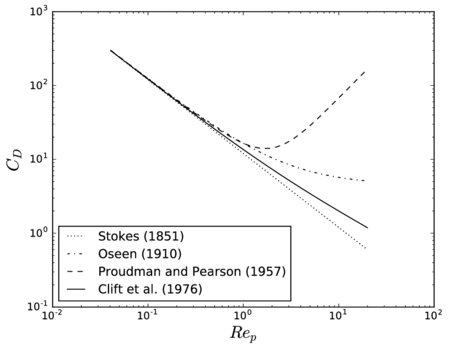
|
| Figure 2: Drag force predicted by different approximations, as measured by the drag coefficient . |
The above expression of the force is only valid for long-term steady motions. Lovalenti and Brady [223] studied the motion of a small sphere immerse in an arbitrary space and time varying flow, although considering the particle small enough, so that the undisturbed flow can be considered uniform over the diameter of the particle. The problem is thus the generalization of the MRE (excluding Faxén terms, as these authors assume flow uniformity; see Section 2.2.1) for small, though non-zero particle Reynolds number. Their analysis is based on a different approach compared to the asymptotic expansion matching used by Proudman and Pearson [284]). In fact, they find an expression for a uniformly valid flow over the whole domain to first order in . The hydrodynamic force on the particle is then computed to first order in by approximating the resulting integrals of the stress tensor. The result is an expression for the steady and unsteady forces at finite Reynolds number. The inertial effects include the steady Oseen correction to the drag, as well as corrections to the unsteady forces like the Basset Force and the added mass force. These corrections confirm the observations from fully-resolved numerical simulations [243] that higher rate of convergence of the particle velocity to terminal conditions (i.e.it varies but is for smoothly accelerating motions where the slip velocity tends to increase) than that predicted by the MRE equation, which is , as predicted by the Boussinesq–Basset kernel. According to Lovalenti and Brady [223]: This fact may explain why experimentalists have measured a steady terminal velocity when the length of their apparatus would not have permitted this if the Basset force was correct..
This change in the decay regime of unsteady forces only applies at long times. For short-time-scale motions the unsteady force from the MRE is accurate. The boundary between both regimes is marked by the time it takes for vorticity to diffuse away from the particle up to the so-called Oseen distance, where inertial and viscous contributions become of the same order. At that point, convection transport takes over as the dominant physical mechanism for the transport of vorticity, explaining the change in regime. From the application point of view it is important to realize whether the flow is dominated by high frequency flows, so that the motion is mainly explained by the MRE unsteady forces, or else the characteristic frequencies of the flow are low and thus the (substantially more complicated) expressions provided by Lovalenty and Brady apply. The key is to compare those characteristic frequencies of the particle's motion with the quantity , the viscous diffusion time, which corresponds to the order of magnitude of the time it takes vorticity to be diffused away to the Oseen length. In other words, the MRE equation applies whenever [224]
|
|
(2.12) |
After a little algebra, this condition can be rewritten as a function of the usual nondimensional parameters as
|
|
(2.13) |
As the value of increases, the condition above may cease to be fulfilled and the form of the history term must be corrected using, for example, the formulation given by Lovalenti and Brady [223]; see also Lovalenti and Brady [224]. In turbulent dispersion, the importance of this correction will not be critical for most flows such that , except perhaps for solid particles in gas. The same conclusion was reached by [211] based on the empirical formulation for the history force of Mei and Adrian [243].
The effect of vorticity
As stated, the derivations in Lovalenti and Brady [223] assume a uniform flow at the scale of the particle. If one allows for some non-uniformity to be present in the flow, additional effects appear. In particular, this allows for a break in the symmetry of the flow on the plane orthogonal to the direction of , which gives rise to lateral forces on the particle that are known as lift forces. Famously, Saffman [299] (with the corrections in [300]) gave the correct expression, to first order in , for the lift force that an isolated, non-rotating particle experiments under constant shear (linear non-uniformity of the flow).
|
|
(2.14) |
where is the slip velocity. This result is valid under the restrictions , and ; where the shear Reynolds number is defined by
|
|
(2.15) |
that is, the particle Reynolds number multiplied by a dimensionless shear rate gradient.
Unfortunately, the typical values for in turbulence are often smaller than those of [364], invalidating the application of the formulation. However, in this case the expression is in fact overestimating the lift force [364] and so, without loss of generality, we may apply the formulation as an upper bound for the remaining discussion.
But the fluid vorticity can arise due to the solid rotation of the fluid as well, also giving rise to a lift. Its low- analytical formula was provided by Herron et al. [164] and reads
|
|
(2.16) |
which has a coefficient about 2x101 larger compared to . This expression is subject to the restriction . Note that and are incompatible and are only strictly valid for their corresponding ideal fluid motions. In fact, Candelier and Angilella [56] have proved analytically that for a particle settling in a solid-body rotation fluid, the lift force can even take the opposite sign as that indicated by Eq.~2.14, which is valid only for pure shear, steady flows. In this case, furthermore, the relative motion is not stationary, due to the migration of the particle in the radial directions.
Indeed, as with rectilinear motion, the relative flow unsteadiness also generates history-dependent contributions. Those have been studied in [60,55] for pure shear (generalizing Saffman's result) and solid-body rotation motions respectively. Nonetheless, the order of magnitude of the Saffmann lift force, compared to the steady drag force gives an idea of the magnitude of this correction. An analogue estimate can be obtained if fluid motion is closer to that assumed in Eq.~2.16.
|
|
(2.17) |
We will thus consider the lift force to be vary small within the range of applicability of the MRE. Nonetheless, one must keep in mind that the correction is orthogonal to the drag force and thus its effect can introduce important systematic changes in the particles' trajectories, especially in flows with a predominant direction. Since the largest values of the shear rate are usually close to the boundaries of the domain, this is very often the case anyway, for instance in internal flows. When considering the flow of particles along ducts, it is therefore important to consider the possibility that the inertial lift force might play a role, except for extremely small particles. In any case, we leave the study of the effect of boundaries for future work, see Section 2.2.6, and thus we will not elaborate this point any further here.
The effect of particle rotation
The linearity of Stokes flow means that, for a spherical particle, rotation and translation are decoupled. Indeed, the combined motion is the result of adding the effects of one and the other, and it is clear that, by symmetry, the relative rotation of the particle alone cannot produce a force in any particular direction. It is however necessary to examine how fast this rotation can be until the first inertial effects appear, invalidating the MRE.
The first-effects of the force modification due to non-zero particle angular velocity were calculated by Rubinow and Keller [294], to zeroth-order accuracy in . This is enough for our arguments, since the MRE assumes this effect to be very small. This formulation predicts that due to the rotation of the particle, there arises a lift force given by
|
|
(2.18) |
where is the angular velocity of the particle. In other words: the Reynolds number defined by the slip velocity produced by rotation should be small enough. The lift force that arises due to the rotation of the particle relative to the fluid is generically called Magnus effect [219].
The condition of having a negligible contribution to the force could then be expressed as a function of the particle Reynolds number associated to the rotational motion, given by
|
|
(2.19) |
where . Note that , and so this is assumed to be very small within the theory of the MRE.
Maxey [238] argues that in turbulent flows the particle will tend to acquire a rotational velocity of the same order as the local shear rate. Taking into account that the first-order rotation-induced effect of inertia is a lift force with a magnitude of order [294], the effect results of order ; more precisely, we have
|
|
(2.20) |
where give the estimation of local shear rate; and being the characteristic velocity and distance of the flow, which is certainly a small quantity by Eq.~2.7.
There are circumstances in which the particle angular velocity might be substantially higher. For instance, a collision against a wall or another particle might transform a good part of the translational energy into rotational energies, leading to high angular velocities, especially for the smaller particles 1. The fact that this force is perpendicular to the direction of translation makes this effect even more important. Nevertheless, collisions are not expected to be too frequent in this regime (see Section 2.2.4), substantially alleviating this effect.
In this chapter we ignore the rotational degrees of freedom of the particle, except for the present discussion, with the argument that these effects are, to first order of approximation, decoupled. Nonetheless, it is worth to consider momentarily what the rotational dynamics of a particle within the range of applicability of the Maxey–Riley regime looks like. Feuillebois and Lasek [128] derived the expression of the instationary motion of a small, rigid sphere spinning in a viscous, Newtonian fluid, providing history-dependent terms that decay much faster than the translational analogues. In the steady-state limit, the equation reads
|
|
(2.21) |
This equation allows us to calculate the rotational relaxation time as
|
|
(2.22) |
from which a rotational Stokes number can be defined (assuming the steady-state forces are dominant)
|
|
(2.23) |
which shows that this Stokes number is of the same order as the translational Stokes number, under the assumption that the fluid time scales are similar. Note that for large Stokes numbers the assumption above that the particles rotation will be of the order of the fluid vorticity most of the time (in fact equal to the local angular velocity or one half of the vorticity in the limit of zero inertia) can be violated, as the particles may not have time to accommodate to the fluid vorticity. In such cases the analysis becomes more involved and it is likely that finite Reynolds number effects must be taken into account for the angular dynamics. Nonetheless, for this order-of-magnitude analysis the present formulation will suffice, especially since the rate at which the steady-state formulation becomes inaccurate is quite slow, and it still yields reasonable results at well past unity, see [219].
(1) Indeed, a fixed percentage of energy conversion from translation to rotation leads to higher angular velocities for smaller particles. Specifically, the rotational kinetic energy is and the translational kinetic energy is . Thus, after a collision we have , for light and/or small particles. Furthermore, this gives ; and the ratio can become quite large.
2.2.2 Finite radius effects
As the particle radius grows with respect to the characteristic length scale of the unperturbed flow the Faxén corrections become increasingly important. Eventually, even these second-order corrections become insufficient to accurately characterize the surrounding flow and the MRE breaks down as an appropriate model. The rate at which this happens can be analysed by taking one more term in the series expansion that leads to the appearance of the Faxén corrections [222] (see also Eq. 8.175 in [91]). It is useful to consider the expression of the drag force as a surface integral to measure the error. The Faxén corrected drag force becomes, after taking one more term in the same expansion considered in [222]
|
|
(2.24) |
Where the is the -th successive composition of the vector Laplacian.
Now, for low , the fluid is expected to present only long-wave length variations across the particle diameter. Furthermore, since our interest lies on the integrated value of such variations, it appears reasonable to assume that the characteristic length scale of the new term is also the particle radius. This allows us to compare its order of magnitude to that of the usual Faxén correction. Let us therefore assume that the effect of the new term is of the same order as that produced by quadratic variation of across the particle diameter. Then, an adequate order-of-magnitude estimate of its value is given by (see, e.g. [245] for a discussion on the estimation of order of magnitude scales)
|
|
(2.25) |
So that the next order correction will be significantly smaller than the classical Faxén correction up to the point when is not small any more (in the limit of quasi-steady Stokes flow it holds exactly). This means that in practice the small requirement will guarantee that the Faxén corrections will make a good enough job and thus the restriction Eq.~2.9, that is, by itself does not appear to be restrictive, but rather indirectly through the violation of . A similar argument can be made with the other forces bearing their corresponding Faxén correction. A significant study supporting this conclusion in the context of isotropic turbulence was provided by Homann and Bec [171], who tested the performance of the Faxén terms for a neutrally buoyant particle in direct numerical simulation (DNS) of isotropic turbulence. Their conclusion was that the first effects of the finite size of the particles were well captured by these terms up to (where is the Kolmogorov microscale). From then on, inertial (finite ) effects quickly kick in.
2.2.3 Nonsphericity effects
No particle is perfectly spherical in reality and thus it is necessary to acknowledge this fact in assessing the reliability of the MRE for predicting the trajectories of real particles. Departure from the ideal spherical shape greatly complicates rigorous analysis and, most often, precludes it completely. The situation is somewhat similar to the consideration of nonsphericity in granular flows using DEM. It is known that its effects are important although only very rough approximations to them can be captured when using only spheres. And while the possibility of using nonspherical shapes also exists, it is greatly limited in practice due to increased numerical costs and difficulties in achieving a good characterization of realistic shapes.
Nevertheless, there has been substantial theoretical progress in characterizing the hydrodynamic interaction of particles of nonspherical shape at low ; see [219] and references therein, [114,59,58]. Gavze [142] derived a generalized version of Eq.~2.1 for a body of arbitrary shape written in terms of its viscous resistance tensors [48]. Within this model translation and rotation become coupled.
Of particular relevance to our arguments is the study of Zhang and Stone [389], who derived the first order asymptotic correction to the unsteady equation of motion of a sphere in quiescent fluid in an amplitude parameter, , of the deviation from an ideal spherical shape using the reciprocal theorem (see, e.g. [152]). Their equations particularize the work in [142] to the limit of weak nonsphericity, in which the coupling between rotation and translation comes in as a higher-order correction and can thus be neglected to first-order approximation.
Specifically, let the particle's surface be defined in polar coordinates around its center as the set of points with coordinates , and such that
|
|
(2.26) |
where is the radius of the equivalent-volume sphere.
Their equation for the hydrodynamic force on the translating particle reads:
|
|
(2.27) |
where
|
|
(2.28) |
and the integral is over the unit sphere , after applying a uniform scaling by its radius over the whole space. Note that represent the exterior unit normals to the unit sphere. The surface of the particle is by construction (although this is not emphasized in [389]) assumed to be star-shaped with respect to its center of mass1. We can then use these results as a conservative estimate of the first perturbations due to nonsphericity to the MRE.
Eq.~2.27 allows us to estimate an upper bound to the magnitude of the corrections to the MRE that are needed to take into account generic (weak) nonsphericity. Let us consider the induced matrix norm on matrices denoted by , based on the usual Euclidean norm for vectors, denoted with the same symbol. Then, for example, the corrected drag force fulfils
|
|
(2.29) |
Similar estimates can be worked out for the other hydrodynamic effects, yielding similar relative orders in their corrections. This bound is related, although a bit less sharp than the one provided by the application of a theorem by Hill and Power [166], which establishes that the magnitude of the steady drag (it only refers to the steady drag force) on the particle lies between that obtained on an inscribed and a circumscribed spherical particles. That is, the center of the circumscribed and inscribed spheres do not have to be the center of gravity. In this case therefore, for steady-state motions, the relative error made by taking the Stokes expression with the average diameter is smaller than
|
|
(2.30) |
In the limit of small corrections to the spherical shape, however, all inscribed and circumscribed spheres tend to collapse to the ones around the center of mass and the result then coincides, for the drag force, with the one provided by the asymptotic technique by Zhang and Stone [389].
(1) In geometry, a body is said to be star-shaped if there exists a point within it such that, for any other point in the body, the straight segment that joins both points is itself fully contained in the body. This appears to be a reasonably weak assumption for approximately spherical particles. In particular, it is much less restrictive than convexity. See [156] for an analytic correction to the added mass force for a (non-star shaped) rough sphere.
2.2.4 Effect of neighbouring particles
The MRE is based on the assumption that the particle is isolated, far away from any neighbouring particles or any other boundary. But, for many applications, such assumption can become too restrictive. Even in the absence of interactions such as electrical potentials or van der Waals forces between the particles, there are still two types of inter-particle influences:
- Mid/long-range hydrodynamic interactions, due to the flow disturbances generated by the presence of all the other particles
- Short-range forces of various types that appear when the inter-particle gaps become very small, such as lubrication forces and inter-particle contact forces
Starting with the long-range hydrodynamic interactions, it is clear that they depend on the configuration of neighbours and their velocities, requiring a statistical approach for a general analysis. Under the low-Reynolds number hypothesis, such influences are linear on the particles' separations (and velocities, including angular velocities), meaning that their spatial decay is slow. Every particle in a suspension produces a disturbance flow around it which, under the hypothesis of a low particle Reynolds number, is accurately represented by the creeping flow equations solution, at least up to a distance comparable to the Oseen distance () [248] from the particle's center, i.e.
|
|
(2.31) |
where the velocity components are Cartesian (with the first component being aligned with the relative flow) but have been parametrized in spherical coordinates, with the radial coordinate (normalized by the sphere's radius) and the azimuthal angle. Note that, by symmetry, the field must be independent of the polar angle, as it is. Eq.~2.31 confirms that the decay of the disturbance intensity is dominated by a linear behaviour, which means that its influence can still be appreciable at significant distances as shown in Fig. 3. In Fig. 4 the average distance to the nearest -th neighbour, as a function of , is shown for reference; for in a random array of spheres. The calculation of this distance is done according to the formulation in [340], that takes into account the space taken up by the finite-size particles and is robust for all values of up to close packing.
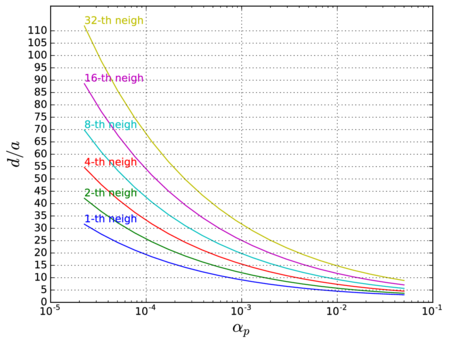
|
| Figure 4: Average distance (normalized by the radius of the sphere) to -th closest neighbour in a random array of monodisperse spheres. |
A description of the flow around a given particle, under the influence of its neighbours, would require the solution of the Stokes equations around all of them simultaneously. And since the solution depends on the velocities of the particles, which are in turn instantaneously determined by the fluid velocity around them, all interactions are completely coupled, making the problem fully multi-body in general. In the dilute limit that we are interested in (we are studying the first-effects of the presence of neighbours), it is, however, possible to give the interactions a pair-wise treatment. This means that they can be calculated as the sum of the interaction between the individual pairs of neighbours with only a small error [23]. Still, the main difficulty lies in describing a representative configuration of relative positions and velocities for a representative ensemble of particles, valid for the general case.
Switching to the short-range interactions, these include two types of forces: the shortest-range hydrodynamic interactions, termed lubrication effects, and the direct contact interactions, that appear once the fluid has been completely squeezed out of the gap between pairs of particles coming into contact. Here too, a statistical analysis seems unavoidable. Fortunately, these effects are more adaptable to the general DEM approach, as these are by definition pairwise, short-range forces that can be naturally included in a contact model. Nonetheless, in some situations it may still be interesting to neglect them completely as:
- The complicated modelling issue associated with the two types of short-range interactions is avoided.
- The computational cost is greatly reduced, as the most expensive parts of the DEM algorithm (force calculation and search) are avoided.
- The time step of the simulation, which is otherwise upper bounded by a fraction of the contact duration, can then be much increased, further reducing the cost.
- It becomes easier to give a completely statistical interpretation to the particles, making it possible to alter the real concentration of particles to speed up the simulations, avoiding for instance the need to consider a realistic number of particles when that is too costly.
We wish to characterize the conditions for which these effects start to become important, causing the MRE to start loosing accuracy in modelling particle-laden flows. Such characterization has been attempted before [116,118] in the context of general particle-laden flows. Specifically, Elghobashi [116] establishes limits on the global solid fraction (the proportion of volume occupied by the particles in the whole domain; see Section 4.8 and Appendix H) for which three-way interactions become important is
|
|
(2.32) |
where is the local solid fraction. This corresponds to an average nearest-neighbour separation of about 1x101 particle radii. This is an oft-cited limit [232,159,206]
We will attempt to enrich the general picture here, surveying the most relevant results and the different aspects to take into account with the ultimate goal of producing a useful guide for practical applications. Once again, we focus on turbulent flows to provide the order-of-magnitude estimates.
Before proceeding, we must make one further remark concerning the scope of the discussion. In some particle-laden systems, the particles may interact forming aggregates, coalescing or breaking. We do not consider these cases here, but rather the case in which the total number of particles and their shape is preserved throughout the simulation.
Hindered settling
In a random arrangement of particles, the added effect of all particles around any one of them can be very substantial, due to the long-range character of the interactions that we discussed above. In fact, the naive summation of the moduli of the disturbances would not work at all for our order-of-magnitude purposes, because of the slow decay of the interactions with distance. Indeed, take the sum of the norms of all the pairwise interactions between the particles inside a ball centred at the target particle and the particle itself, which bounds the contribution of the particles considered above. By considering a sequence of balls of growing radii, one obtains a sequence of sums that, due to the linear decay of the forces with distance, does not lead to an absolutely convergent series, because the number of terms grows with the third power of the radius in a statistically homogeneous distribution. Thus, such straightforward strategy fails to produce any bound at all.
This difficulty was overcome by Batchelor [23], who was able to rigorously calculate the (ensemble) average, to first-order in the solid fraction, of the effect of a stable, random uniformly distributed suspension of identical rigid spheres on the settling velocity of any given particle. This author used an ingenious method in which known averaged quantities were used to cancel out the slow varying contributions exactly, reducing the remaining terms to rapidly varying quantities that could be calculated, to first order in the concentration, based on the interaction of the two closest particles only. The result of his analysis can be written as
|
|
(2.33) |
where is the terminal velocity of the target particle when isolated, the actual settling velocity of the particle in the suspension, is the solid volume fraction and is the settling coefficient, which under the particular assumptions of the theorem is ; and . This result is based on the further assumption that the probability distribution of the distance between pairs of particles is uniform. A similar expression has been derived for polydisperse suspensions [24,93], yielding smaller values for . For instance, for both small spheres surrounded by a suspension of larger spheres or the opposite situation (See [100]). Therefore, one may use Eq.~2.33 as a conservative order of magnitude of the first effect of the presence of neighbouring particles in sedimentation of statistically homogeneous suspensions. Note that in this case ( is negative) the presence of other particles tends to slow down the target particle as it sediments. This is true specifically because of the assumption of having a uniform suspension that can be treated as unbounded, since non-uniformity often leads to a reduced resistance and thus an increased settling velocity with respect to an isolated particle, as will be shown below.
Drag modification
Another relevant theoretical result can be taken as a reference to study the effects of the presence of a random array of particles around a target particle for the calculation of the drag force, which is enough to assess first-order effects due to the surrounding suspension. The theory is based in the asymptotic analysis of the hydrodynamic forces in the low Reynolds number and solid fraction limit, which is relevant to the present discussion. It was put forward by Kaneda [189] and experimentally verified up to solid fractions of around 4x10⁻² for small Reynolds numbers based on Brinkman's screening length, , as the simulations for higher values of were found to be prohibitively expensive, in [167].
The derivations by Kaneda were performed for simplicity under the hypothesis , although the resulting expression is shown to have the correct asymptotic behaviour at the opposite limits and . In this work it is argued that the first effects of inertia (see Section 2.2.1) and those of the nonvanishing solid fraction cannot be treated independently as both are inextricably linked for all but essentially zero Reynolds numbers. The expression for the modified drag is
|
|
(2.34) |
with
|
|
(2.35) |
where 1 is a nondimensional constant such that (when ) and where is the usual Stokes drag; and
|
|
(2.36) |
Note that
|
|
(2.37) |
Which, as stated, recover the first order correction due to Oseen for the drag force at (and thus ), see Eq.~2.11, and also the classic expression by Brinkman [49], at .
Figure 5 shows the magnitude of the correction coefficient for a wide range of solid volume fractions, for different values of . Note that the correction to the drag is significant, even for very small Reynolds numbers if the solid volume fraction is greater than 1x10⁻³, in accordance with the rule of thumb of Eq.~2.32, and it still appreciable past the 1x10⁻⁴ mark.Although Kaneda's result applies to arrays of fixed spheres under a uniform background flow, it clearly reflects the inextricable relationship between the low-Reynolds number and low-concentration hypotheses through the dimensionless number . This number can be understood as the quotient between two length scales:
|
|
(2.38) |
where is the Oseen length (distance from the particle at which inertia becomes as important as viscosity) and (distance from the particle at which the Stokesian disturbance caused by it switches from a linear to a cubic-order decay due to the presence of neighbours). The physical interpretation of the two regimes in Eq.~2.36 goes as follows: when is very small (), inertial effects enter much before the Stokesian disturbance has been screened by other particles and thus their influence is dictated by finite- effects. On the contrary, if , the influence of distant particles is screened before it can reach the target particle, and only the effect of Stokesian flow disturbances is felt.
Finally, note that the concentration dependence of the drag force is proportional to the square root of the solid fraction, to first order, under the assumption of having a small Reynolds number based on the system size. This contrasts with the result by Batchelor discussed in Section 2.2.4, under which the resistance depends linearly on the solid fraction under the same hypothesis. The reason is the hypothesis of a fixed bed used by Kaneda, which constraints the possibilities that the particles have to accommodate to the resistance, causing it to be more important. The hypothesis of a free bed adopted by Batchelor is more relevant to the behaviour of a cloud of particles suspended in a fluid [92]. Nonetheless, the description of the two regimes studied by Kaneda does remind us that the assumption of having a small Reynolds number used by Batchelor is actually tied to the condition of having a large enough solid fraction to make sure that , a condition that was not explicitly stated by this author.
Recently, Pignatel et al. [278] have experimentally studied the transition between regimes of a falling (finite) cloud of particles. In this case, the Oseen length scale is compared to the clouds initial diameter. Furthermore, a Reynolds number associated with the cloud's length scale is also considered. Several regimes are identified, but what is most interesting to the present discussion is their identification of the Stokes regime (Batchelor's hypothesis) for , . We will come back to considering sedimenting clouds in the proceeding paragraphs, which address inhomogeneous suspensions.
Clustering
In reality, the assumption of homogeneity in the spatial distribution of a suspension is rarely fulfilled. Instead, it is often the case that the particles approach each other forming more or less defined clumps, a phenomenon known as clustering. This is observed very prominently in turbulence, where inertial particles tend to concentrate in filament-like structures causing the solid fraction to fluctuate strongly within the domain [127,305,350,262].
A number of theories have been proposed to explain these inhomogeneities, and it seems that, rather than a single mechanism, there are several [309,44,157], and their relative importance may depend on several factors, including the particle Reynolds number and, especially, the Stokes number. The most well-known of these mechanisms consists in the progressive expulsion of heavy particles from high-vorticity regions into straining-flow regions [112] as a result of their inertia. This is known as the centrifuge mechanism and it has been well documented both from simulations [239] and experiments [305]. In other words, the inhomogeneities arise because the particles spend more time in high-strain regions than in high vorticity regions, so they tend to concentrate there. Such oversampling of regions of the flow with specific properties is generally known as preferential concentration [323,145]2 in the literature.
While the preferential concentration effect is the most predominant at small Stokes numbers [45], other mechanisms become important as grows. For instance, the sweep-stick mechanism [149] consists in the tendency of particles to move away from regions of high accelerations and stick to the low-acceleration zones. The sweep-stick mechanism becomes important at around and higher (inertial range).
Another effect that becomes important at finite Stokes numbers is the so-called sling effect [122] which develops in intense turbulence. This effect is caused by rare events where very large gradients develop, producing jets of particles that are ejected from the trajectories defined by the streamlines of the vortices from which they come, just as a sling does with a stone. The ejected particles can enter regions where the local suspended particles have significantly different velocities, rendering the particles velocity field (the hypothetical field formed by the trajectories of an infinitude of particles taking up all space) multivalued, a phenomenon known as caustics [367]. These caustics are responsible for an important increase of the collision rate of particles, and is currently believed this plays a crucial role in explaining the fast rain initiation times in turbulent warm clouds [122,123].
Other mechanisms for the appearance of inhomogeneities are turbophoresis [257] and clustering related to boundary layers [234], although we will stick to homogeneous, isotropic turbulence in our discussion for the sake of simplicity. An important and perhaps surprising fact about the clustering effects is that they are known to continue below the smallest scales of the flow, the Kolmogorov microscales in turbulence. Indeed, inertial particles tend to cluster forming multifractal structures [26] at sub-Kolmogorov scales, in a process that is still not fully understood. Furthermore, this phenomenon is not exclusive of turbulent flows, and can even be produced by random, uncorrelated fields that contain a smallest length-scale, as shown by Bec [25].
Important efforts are being made to characterize the phenomenon and some statistical models, and the development of physical theories to gain insight into clustering phenomena are currently being developed, along with predictive models that are yielding correct qualitative as well as quantitative predictions [382,381,73,131,157]; see [157] for a review. These models contain a number of assumptions and simplifications that limit their range of validity. Recently, Bragg and Collins [44] reviewed some of these formulations, recommending the one by Zaichik and Alipchenkov [381] as the most comprehensive and robust over a wide range of values (see below).
Nonetheless, there remain a number of open questions and inconsistencies in the literature that need to be addressed. For instance, there is a significant consensus that the strength of clustering peaks at [253,178], However Sumbekova et al. [328] concludes that the level of clustering, measured using a Voronoï tessellation of space, is most strongly related to the Taylor Reynolds number, less so to the average particle volume fraction and negligibly on the Stokes number. Moreover, Uhlmann and Chouippe [349] has found that clustering scaling seems to depend on the mode in which it is measured.
Understanding the physical mechanisms that govern the appearance of clustering is of extraordinary importance, not only due to its relevance to the assessment of the validity of the single-particle theory (which includes the MRE), but also in understanding the statistical distribution of particles in space, statistics on the flow properties being sampled (of relevance to the simulation of chemical reactions, for example) and the prediction of the collision rates (of relevance to the study of initiation of rain and snow, for example). Of direct relevance to the present discussion is the study by Aliseda et al. [4], where the settling velocity of spheres was measured experimentally in a turbulent channel flow. A notable increase in the settling velocity was observed with respect to quiescent fluid conditions, especially for Stokes numbers on the order of unity. Furthermore, this velocity increased monotonically with the overall volume fraction, indicating the effect of three-way coupling. A phenomenological model based on the idea of particle clusters locally altering the average velocity seen by its constituent particles turned out to explain the observations very well. It is remarkable that the whole study was performed under volume fractions well below the limit given in Eq.~2.32, which clearly demonstrates the limitations of the single-particle paradigm.
The estimates provided in Section 2.2.4 were derived under the assumption of an unbounded array of particles characterized by an average solid fraction under the hypothesis of having a homogeneous suspension. Therefore, the existence of significant inhomogeneities as those caused by preferential concentration in turbulent flows, invalidate the theory and the derived estimates. Aliseda et al. [4] proposed a phenomenological model to explain the effect of preferential concentration in a turbulent suspension of settling particles. They observed that the average settling velocity of the particles belonging to a cluster was reasonably well predicted by Eq.~2.33, with
|
|
(2.39) |
where is the volumetric shape factor [285], an order-one constant that depends on the shape of the cluster and is equal to one for spherical clusters and is the characteristic size of the cluster. This formula was derived under the hypothesis of quasi-steady Stokesian flow around the cluster. That is, this work is concerned with the low-Reynolds regime
Interestingly, this model was theoretically ratified by Jabin and Otto [181] under similar conditions, though no mention is made in their paper of the previous investigations by Aliseda et al. This remarkable work seems to have remained relatively unknown, perhaps because of this omission. This work refines the picture sketched by Aliseda et al. by
- Rigorously proving the following relation
(2.40) - Establishing the existence of a critical, minimum number of particles () that must be contained in the cluster, so that it behaves as a macro-particle and where Eq.~2.39 applies. The macro-particle argument was precisely the one used in [4].
- Establishing a lower bound to the time scale in which the particles will not come close enough to invalidate the model, which is the time scale of the time taken by the cluster to settle a distance equivalent to . This point is fundamental in proving that the macro-particle model is stable for a sufficiently long time to apply the theory effectively.
where is an unknown constant and where is the average separation between the particles in the cluster. This expression is equivalent to Eq.~2.39 in the regime (), as it can be immediately shown using and .
Further support to this model can be found by using an argument due to Zaichik and Alipchenkov [381] (ZA henceforth). Note that this is the same work describing the model advocated by Bragg and Collins [44] for the description of clustering in turbulence, mentioned above. ZA used the theory of Batchelor [24], a generalization of that discussed in Section 2.2.4 allowing for non-uniform spatial distribution of particles, to provide an expression for settling coefficient in the much more general setting of isotropic turbulence. The general expression reads:
|
|
(2.41) |
where is the radial distance normalized by the particle radius ; , , and are the mobility functions of the particle pair [24] and is the radial distribution function (RDF), defined as the ratio of the probability density of particle pair relative to the same quantity in a uniform suspension, see, e.g., [380].
In simple words, the RDF gives, assuming a particle is found at a certain location, the average number of neighbours found at any given distance from the former, expressed as a proportion to the average number found at that distance in a homogeneous distribution. Note that this is an infinitessimal quantity. The latter can be approximated as
|
|
(2.42) |
where the number density is the number of particles per unit volume and is the ball of (nondimensional) radius centred at the particle.
The RDF is often employed in the fundamental study of turbulence dispersion [310,26]. This function would be exactly equal to one for a statistically homogeneous distribution. When a certain degree of inhomogeneity is present, one observes peaks in its value at distances of the order of the characteristic distance of the inhomogeneities (the diameter of the clusters, say). Typically, the RDF asymptotes to one at infinity, as homogeneity is often attained at large enough distances. This is roughly the case for many physical systems, including particle suspensions in turbulence [381] and the molecules in an ideal gas in thermal equilibrium [161] and even the distribution of matter in the universe [347].
The different terms in Eq.~2.41 can be identified as the effect of the particle-pair interactions (), the effect of preferential concentration () and the effect of backflow (the resistance caused by the displaced fluid raising due to the settling of the particles cloud).
Therefore, Eq.~2.41 provides a means to calculate the effect of generic inhomogeneities on the settling velocity of the individual particles. Note that it can also be interpreted as the effect on the drag force (since in a time-averaged sense both notions are one-to-one related) of the presence of neighbours in remarkably general conditions, and in a time-averaged sense. This is of interest to produce a first set of estimates for the effect of neighbouring particles in a wide range of situations involving a predominant drag force and arbitrary distribution of particles. We believe it can provide an order-of-magnitude guide for engineers that wonder about the magnitude of this effect. Nonetheless, the whole theory is subject to the assumptions underlying Batchelor's theory of sedimentation, and thus the restrictions mentioned at the end of Section 2.2.4, defining the Stokes regime for the whole cluster, apply here too.
The key is thus to provide an expression for to calculate the settling coefficient. ZA distinguish between three different regimes, valid for heavy particles ():
Vanishing inertia () with no turbulence In this case there is no clustering and thus , which leads to the same expression derived by Batchelor in [23], where a random, uniform distribution was assumed. In such case, the settling coefficient is given by Eq.~2.33.
Vanishing inertia () In general, in a turbulent flow field the particles interactions produce a drift velocity of the non-inertial particles towards one another [382,73]. Taking this drift into account modifies the RDF (see [381]), leading to . That is, there is a small increase of the settling velocity that cannot however compensate the hindering effect completely, making the particles settle slower than isolated, by an amount that is about 4x101 less than that corresponding to a laminar settling situation. In terms of order-of-magnitude arguments this is in any case a negligible correction.
Finite but small inertia () In this case, the RDF is derived from the equations presented in [381] for low inertia particles, based on a power-law model for the RDF:
|
|
(2.43) |
where is defined so as to guarantee continuity and and depend only on the Stokes number. can be interpreted as a characteristic size of a cluster, since beyond this length the RDF becomes uniform [381]. While this formulation is only strictly valid (within the ZA theory) at distances smaller than the Kolmogorov micro-length scale , they use it anyway, warning of its exclusively qualitative value beyond that point. But since we are interested in distances of only up to the order of a few times this distance (the effect at larger distances would be more appropriately dealt with through a two-way coupled approach), and taking into account the excellent agreement of ZA's model with the results reported in [178], fitted from DNS results in the range , we will consider it reasonable for order-of-magnitude arguments.
Moreover, ZA point out that for heavy particles, with (although, judging from their [381], this argument could be extended to ), one has and so using Eq.~2.43 we can write
|
|
(2.44) |
which can be rewritten as
|
|
(2.45) |
where ( corresponds to in [381])
|
|
(2.46) |
The values of and are reasonably approximated in by [381]
|
|
(2.47) |
Large inertia () In this case the outweighs by a large margin, since the small disturbances caused by the surrounding neighbours have a relatively small effect on the sluggish, heavy particles. Therefore it is possible to take 3
|
|
(2.48) |
where now the radial coordinate () is normalized by the Kolmogorov micro-scale. ZA provide a set of stochastic, probability conservation equations that can be numerically solved to determine .
The formulation by ZA is reviewed and compared to the alternative formulation by Bragg and Collins [44], who, while not addressing the issue of settling, compare it to the alternative formulation of Chun et al. [73] and give a synthetic review of the most important physical mechanisms that explain the development of inhomogeneities in particulate suspensions in turbulence. Furthermore, these authors propose to introduce a change in the original formulation by ZA to include the non-local diffusion effect, as had already been applied by [73]. This mechanism is due to the over-sampling of strain vs. rotation regions by inertial particles. Based on an analogy between the two formulations, they were able to apply the same modification to the model by ZA, yielding more accurate results when compared to experimental results for all Stokes numbers, but especially for . For this range of values of the modification is reduced to modifying the value of in the model of Chun et al. by dividing it by the value . And since in this regime the values for for both models are extremely close, we can apply the same multiplicative factor to the value obtained from Eq.~2.47, obtaining a corrected approximation for small Stokes numbers. Doing so results in a much more perfect coincidence between the ZA theory and numerical results for at small values of (see Fig. 6 to appreciate the corrected level of matching).
Still, for larger values of the full ZA formulation must be solved numerically. This is cumbersome and does not allow us to obtain explicit analytical estimates as we would like. Furthermore, Ireland et al. [178] have shown the estimation of ZA to be accurate only up to , even when the non-local diffusion correction is applied due, they argue, to its poor prediction of the relative velocity statistics at .
We have thus taken a different path at . We use the fitted expression for given by the former authors in this regime. It is again based on the power-law model of Eq.~2.43, where the and are empirically derived. Evidence supporting the power-law scaling of the RDF has been presented for [288,178].
Once again, the coefficients and are functions of the only. This hypothesis can be seen to be reasonable up to and is independent (or only weakly dependent) of the Reynolds number, at least for the range of Reynolds numbers investigated so far [178]. A set of values of and , as a function of where obtained from DNS results and plotted in [178]. We provide a simple fit to this data points from the digitalized images of these plots, see Fig. 6. We found that a very convenient model for our fit was given by
|
|
(2.49) |
which is proportional to a lognormal distribution probability density function. The optimal parameters and were found to be
|
|
(2.50) |
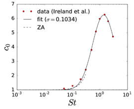
|
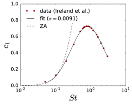
|
| (a) | (b) |
| Figure 6: Fits for the and as a function of . The data were extracted from the digitalized Figure 22 in [178]. The continuous curves correspond to the fits in Eq.~2.49. The values of in parenthesis show the root mean square error of the approximation. | |
Now, using Eq.~2.43 and stitching together the corrected version of ZA with the fits above for and we are able to produce an explicit analytic formula for the settling coefficient that can be used to establish the first-effects of the influence of the neighbouring particles in a situation were non-uniform suspensions are to be expected, due to turbulence. This formulation is furthermore limited to heavy particles, but can be used as a conservative estimation for lighter particles while a more complete theory is still unavailable. The condition for neglecting the collective effects of neighbours then becomes, based on Eq.~2.33, or, assuming a maximum value for the acceptable influence at 1 change in the settling velocity, the maximum solid fraction can be expressed as
|
|
(2.51) |
where has the expression of Eq.~2.45 and where the expression for and can be taken from Eq.~2.47 (dividing by 4.2x10⁻¹) for small values of and using Eqs.~2.49 and 2.50 for larger values. The behaviour of as a function of have been plotted in Fig. 7a for different values of the relative density.
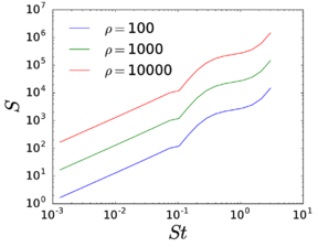
|
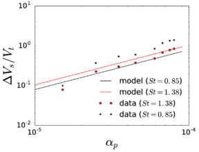
|
| (a) Settling coefficient as a function of the Stokes number using Eq.(2.45) with Eq.(2.47) for (with the non-local diffusion correction) and Eq.(2.50) for larger values. | (b) Estimation of the settling velocity using the same criterion with the data from [4]; the dots correspond to empirical data from [4], digitalized from Figure 17 in [381]. |
| Figure 7: Effect of the Stokes number on the settling velocity based on the theory of Zaichik and Alipchenkov [381], with corrections from Bragg and Collins [44], Ireland et al. [178]. | |
Note that the curves in Fig. 7a show a change in concavity at around toward a positive one. This is unexpected, as it has been empirically observed that tends to peak at one, and then monotonically decrease for larger Stokes numbers. This signals a clear flaw of the present model. Nonetheless, we believe the predictions are much more likely to be correct up to , as it is at around this point that the first signs of Reynolds number dependence in the and values are observed [44]. Therefore, Fig. 7a should be treated with caution and probably only for values of the Stokes number below one. Beyond this point, the value attained at one could be used as a conservative upper bound, as we know the maximum clustering is expected at around this point.
A final remark about this subject is the following. The power-law model for the RDF is supposed to be valid all the way down, below sub-Kolmogorov scales, in accordance with DNS results for monodisperse suspensions. However, such model might suffer from the effects of a certain level of over-idealization. Chun et al. [73] studied this issue theoretically for small-inertia particles and concluded that arbitrarily small differences between the diameters of the particle pairs lead to the appearance of a cut-off distance below which the RDF approaches a constant. This observation goes in the direction of moderating the amount of clustering expected at very small separations in real-world situations and should be kept in mind when interpreting our results, since our analysis has been limited to monodisperse dispersions.
Effect of collisions
In this work we are mainly interested in CFD-DEM methods, where the MRE is enriched by the addition of contact forces to its RHS. In such a case the effect of collisions is naturally accounted for and the need to estimate the effects of its neglect diminishes. Nonetheless, in practice there are many situations in which it becomes advantageous to turn off inter-particle interactions:
- Removing interactions eliminates the smallest scales in the system (as long as the particle-wall interactions are also eliminated), which leads to the possibility of using much larger time steps
- It can be difficult to accurately model inter-particle interactions, due to uncertainties in the rheology involved
- The number of particles is sometimes made smaller in the simulation compared to the real system to reduce the overall cost, which alters the collision frequency artificially, rendering the effort pointless
- The overall computations become simpler and, thus, cheaper
Therefore, it is interesting to study under what conditions inter-particle interactions can be eliminated without incurring in serious error.
The evaluation of the first effects of collisions must be based on a statistical analysis because any useful characterization of a typical collision has to consider both the magnitude and angle of the approaching particles' velocities, which are stochastic variables by virtue of the chaotic nature of turbulent flows. Such characterization is challenging, as it must be derived from local and history-dependent knowledge about the flow and the particles, including (but not limited to) the modelling of clustering that we discussed in the previous section.
The problem of estimating the rate of collision is central to the study of rain formation in clouds and, for a long time, it has been (and continuous to be) a topic of constant developments motivated by this problem and others [288, 123, 70].
For our purposes, though, we can use relatively crude estimates to bound the importance of these effects that can be useful for engineering considerations. In this regard, Loth [216] has established that inter-particle collisions have a negligible effect to the overall trajectories of the particles if the average inter-collision time is substantially larger than the particle relaxation time. This criterion naturally gives rise to the definition of a collisional Stokes number as
|
|
(2.52) |
where is the reciprocal of the average collision rate, . The above criterion thus requires an estimation of the collision rate, valid in as wide a range of regimes as possible.
In order to do so, one may use the following formula, that relates the collision rate of two generic neighbours, labelled , with their expected relative velocity:
|
|
(2.53) |
where
|
|
(2.54) |
where is the swept area formed by the projected silhouette of the two particles onto the plane orthogonal to , and are the respective radii and is the number density of the species of the particle . With this formula, the problem reduces to the determination of the expected number density (which can be obtained from the RDF) and the expected relative velocities, where the value of can be determined as a function of these values for spheres.
Loth [216] distinguishes between two sources of collisions, corresponding to different causes for the existence of the relative velocity: those due to turbulent fluctuations of the flow and those due to the different terminal velocities of particles of different terminal velocities under the influence of gravity.
For the case of gravity-driven settling, one can estimate the collision frequency experienced by a particle by calculating the swept volume per unit time of its neighbours as seen from a frame of reference moving with the average speed of the particles ensemble. Assuming monodispersity, the average number of collisions in a given time interval can be calculated as , corresponding to a cylindrical volume of base and height , where is an average relative velocity of a particle with respect to its surrounding ensemble. For small differences in the settling velocity, due to weak polydispersity this yields
|
|
(2.55) |
and the equation is valid to first order in , where is the range in diameters normalized by the average diameter.
The turbulence-driven collision frequency has been intensely studied [199,383,358]. Here we follow Loth [220] who bases the analysis on two limiting expressions are valid for two extreme regimes: the very low and very high Stokes numbers. For very low Staffman and Turner [301] derived the following expression, which has been validated in numerical simulations in the limit of very small Stokes numbers [331].
|
|
(2.56) |
where represents the usual Stokes number based on the Kolmogorov microscales.
At the opposite extreme, in the so-called uncorrelated regime, the following expression can be derived [220]
|
|
(2.57) |
where is the Stokes number based on the eddy turnover time and where is the lateral integral scale of the turbulent flows [280].
A simple approximation was proposed by Loth [220] to bridge both regimes in between (intermediate regime). This approximation is rough but sufficient to provide a first estimation of the importance of tracking collisions in dilute particle-laden simulations. The result is
|
|
(2.58) |
For more accurate estimates see [331,383,71], where more advanced models for the collision frequency in the intermediate regime are discussed.
In order to unify most criteria, we can take, as a first approximation, the minimum of the two definitions Eqs.~2.55 and 2.58, so that the condition to be able to neglect collisions in turbulence becomes
|
|
(2.59) |
(1) The asterisk has been added to avoid a symbolic clash with the settling coefficient, .
(2) For particles lighter than the surrounding fluid, such as air bubbles in water, the inverse type of oversampling is observed [5], as expected.
(3) Note that there appears in Equation 79 in [381] the lower limit of the integral is 0.0. Note however that this is inconsequential, since there is no contribution of the integral between 0.0 and because no particle centres can be found closer than .
2.2.5 Small-size effects
In theory, the validity of the MRE should tend to be fully attained in the limit of a vanishingly small particle radius. Indeed, Eqs.~2.7-2.9 can all be fulfilled by making small enough. Small particles are thus the realm of the MRE. However, the implicit assumption of the applicability of the Navier–Stokes equations to the continuous phase in this limit is in fact flawed because the continuum hypothesis fails at sufficiently small sizes. In this section we look to determine the order of magnitude of the lower acceptable limits for the particle size for which the MRE still applies. Since the behaviour of a fluid near the referred limit is different for gases and liquids, we treat each one separately, keeping in mind mainly water and air as the archetypical examples.
Gas flow
At large scales, the evolution of gases is well described by the Navier–Stokes equations, which are based on the hypotheses of continuum and of pointwise thermodynamic equilibrium (or at least quasi-equilibrium) that lead to the linear stress-strain rate relation [135]. The progressive deterioration of the validity of this assumption as the length scales shrink manifests itself as the so-called rarefaction effects. These effects arise due to the growing mean free path (the average distance that the molecules travel between successive impacts [313]) relative to the particle dimensions and the corresponding lower frequency rate of collisions 1. The Knudsen number, , specifically quantifies this phenomenon and is defined as
|
|
(2.60) |
with the mean free path (MFP) and the representative physical dimension of the flow, which is usually taken as the particle radius in this context. In reducing the particle radius, the first rarefaction effects to be expected to appear are related to the breakdown of the no-slip boundary condition [193], which is used to derive the MRE. Let us thus investigate the issue a bit further.
Upon impacting on a solid wall, the gas molecules exchange momentum in the tangential direction in other than idealized conditions. If all the reflections were merely specular (symmetric with respect to the surface average normal), there would be no average exchange of tangential momentum and one would have slip boundary conditions. For most materials, however, this is not the case [21], resulting in a net tangential momentum exchange. The main mechanism for such exchange is mediated by the molecular-scale roughness on the wall, that randomizes the reflection angle of the particles, absorbing a part of the statistical bias in the tangential component of their momentum. The exchange is statistically systematic as long as the average relative velocity between gas and wall is nonzero.
As a result of the solid movement, near to the wall, the gas becomes statistically out of equilibrium, because there is a large number of molecules biased toward the wall velocity. This spatial shift in the mean velocity is rapidly homogenized over the neighbouring particles, moving away from the wall. This process is nonlinear (unlike the transmission of the macroscopic momentum, which, at close distances from the wall is linear) and spans a few mean free paths. Such out-of-equilibrium region is known as the Knudsen layer [193]. We can conclude that the assumption of no-slip boundary condition at the solid wall must introduce an error of the order of , that is, proportional to .
While such an error is the manifestation of the onset of non-continuum effects, the continuum model still has application for a range of Knudsen number values after these effects are first noticeable. This can be achieved through a generalization of the boundary conditions to partial slip (see [390] for a recent review) if is small enough. The set of low conditions for which this strategy is appropriate is called the slip regime. If one pretends to extend the applicability of the MRE to this regime, it is evident that one would need to modify the equation to adapt to the replacement of the no-slip condition. Let us look into this.
At the very small particles limit that we are examining, the particle Reynolds number is expected to be extremely low, and so is the Stokes number (unless one is interested in high frequency oscillations, see [79]). This means that the prevailing force is the Stokes drag in this region (see Section 2.3). So to estimate the order of the error introduced by the use of the MRE in this range, we will first look at the drag force corrections for the low-Knudsen number limit (weak non-continuum effects), neglecting for now the other forces.
As previously mentioned, the Navier-Stokes equations must be considered along slip boundary conditions. The simplest and most commonly used model is given by the Navier–Maxwell–Basset formula [390], that assumes the tangential slip velocity at any surface point on the sphere to be proportional to the local tangential stress. That is:
|
|
(2.61) |
where is the local tangential stress and is known as the Basset slip coefficient, in general ranging from zero (perfect slip) to infinity (no-slip conditions).
The corresponding drag force on a sphere moving in uniform motion through an otherwise quiescent infinite fluid is (see, e.g. [283])
|
|
(2.62) |
since is a positive number.
In 1879, Maxwell derived such boundary condition from the kinetic theory of gases under isothermal conditions (we will assume isothermal conditions are a good approximation for the applications we are interested in). Those are given by the following expression, which relates the coefficient with the mean free path from the kinetic theory of monatomic gases in isothermal conditions.
|
|
(2.63) |
where is the tangential momentum accommodation coefficient 2. This parameter is defined as the proportion of molecule collisions that result in a diffusive reflection (as opposed to specular) over the total. A molecule is said to undergo diffusive collision when its incidence angle (with respect to the wall's normal) is uncorrelated with the reflected angle, which is randomly distributed. On the contrary, specular reflection means that both incident and reflected angle coincide. The average of the tangential momentum exchange over a number of diffusive collisions equals the average incident momentum, since the average over the reflected momenta has null mean (no-slip). In contrast, the averaged momentum exchange for a number of specular collision has zero mean, and the momentum transfer is null (full slip). The average in reality is somewhere in between these extremes. The value of depends on the gas and the surface material and finish, but experimental evidence shows to be between 2x10⁻¹ and 8x10⁻¹ (or ), with the former corresponding to specially treated, ultra-smooth surfaces and the latter to most practical surfaces [133]. Maxwell model is derived, by taking the first order (in ) effects into account, and thus its validity is bounded below by ; the so-called slip regime [193]. Higher order approximations have been derived, but this is unnecessary for our purposes.
Substituting these numbers into Eq.~2.62, we come up with the approximate requirement that , which imposing our accustomed one percent error bound reads
|
|
(2.64) |
for typical (most) surfaces. Taking the mean free path of atmospheric air as a reference, this means the particles radius should be larger than about 3 μm . Note that this requirement can become more strict for highly polished surfaces, dropping to for , putting the minimum radius at a ten times larger value.
While small-frequency conditions are the most relevant for a majority of applications with low , it is still possible that higher frequencies arise, either due to the flow's own turbulent fluctuations or due to external forces, such as forced vibrations due to the workings of certain machinery etc. While an analysis analogous to that of Coimbra and Rangel is not available yet for small , a recent paper [376] addresses the case of imposed harmonic motion on the particle submerged in quiescent gas (rather than the perhaps more representative case of forced motion on the fluid and a free particle treated by the former authors) for small . We consider this case to be representative for unsteady motion in low conditions, at least for order-of-magnitude arguments. In the referred paper, expressions are provided for the asymptotic limits in which we are interested, that is, the limit of , where is a nondimensional frequency defined as (see [376])
|
|
(2.65) |
where is the molecular collision frequency, is the characteristic frequency of the relative motion and is a Stokes number 3, defined as
|
|
(2.66) |
The first of these nondimensional numbers measures how the characteristic length scales of the system compare to the mean free path of the gas, which is related to the statistical convergence of the spatial homogenization, while the second number measures the ratio of the characteristic frequencies to the molecular collision frequency, which is related to the temporal homogenization.
Yap and Sader [376] provide the expression for the force in the slip regime, along with the force in the fully no-slip limit (which can be found, for example, as a solved exercise in [202]). The ratio of the amplitudes of both forces (with the no-slip case in the denominator), which we refer to as , provides an adequate measure of the distance from the MRE range of applicability, to first order in the . For conciseness, we do not reproduce its complicated expression here, but instead directly plot it in Fig. 13. In it, we highlight the one percent and ten percent error curves. Note how the force decreases both as and grow, as the momentum transfer at the particle's surface weakens.![Ratio of force calculated as in [376], valid for small Kn and β, to the magnitude of the force calculated with the MRE, valid under the continuum, no-slip conditions on the surface of the sphere.](/wd/images/thumb/8/8e/Draft_Samper_307425316-monograph-graph_force_abs_quotient_beta.png/300px-Draft_Samper_307425316-monograph-graph_force_abs_quotient_beta.png)
|
| Figure 8: Ratio of force calculated as in [376], valid for small and , to the magnitude of the force calculated with the MRE, valid under the continuum, no-slip conditions on the surface of the sphere. |
Note that the intersection of the graph with the plane recovers the steady-state asymptotic behaviour discussed above. For the case shown, , consistent with [376]. Such value comes as a result of refined gas-kinetic simulations, which correct expression Eq.~2.63 and taking , see [21]. While the final value is about twice as big as the typical values expected following the above arguments, its order of magnitude is well within the mentioned limits and thus consistent for this matter.
In Fig. 8 we have limited the range of and so that is bounded above by 1x10⁻¹ since, as mentioned, the validity of this formulation is confined to small values of and . Nonetheless, within these restrictions, we have chosen the range of values for in Fig. 8 to cover all relative motions that could be driven by turbulence within the range of applicability of the MRE, but leaving out extremely large frequencies that would have to be excited by some external force. Indeed, the modified Stokes number can be related to Eq.~2.4 by using the estimate , with the characteristic time of the relative motion (which in turbulence-driven flows will be governed by the fluid's small scales motion). This gives
|
|
(2.67) |
The order of magnitude of the coefficient of can reach values of over 1x10³ for some materials (e.g.heavy metals suspended in air). Thus, roughly speaking, the graph covers , well beyond our range of interest (see Table 1).
In summary, at the small-size limit that we are analysing it is unlikely to encounter large Stokes numbers due to the tiny inertia of the particles. Nonetheless, one should keep in mind that under unsteady circumstances, the low limitation is intensified, so particular attention must be paid to these situations if the MRE is to be applied.
Liquid flow
The molecules in a liquid are typically much closer than in a gas under the same conditions. Specifically, while the typical mean free path in atmospheric air is in the order of ten molecular lengths, the same distance is only in the order of a single molecule in water [134]. This explains the low compressibility of fluids with respect to gases. The result is that the concept of mean free path, and thus , is less useful for the theoretical characterization of liquids than for that of gases. Furthermore, the hypothesis of low density gas, where the molecular collisions can be regarded as binary and instantaneous, which is at the heart of the classical statistical treatment of gases does not apply. The result is that the molecular theory for liquids is much less developed than that of gases and, for example, a reliable analysis of the breakdown of the no-slip boundary condition is not available yet [134]. Another consequence of the higher density of gases is the change in the order of appearance of small-size effects (see [249]; compare Figures 1 and 4). Indeed, here non-continuum effects come before thermodynamic non-equilibrium effects. That is, statistical fluctuations become significant before the no-slip condition breaks down. These statistical fluctuations are due to a finite number of molecular collisions, leading to an erratic movement of the particles known as Brownian motion. Indeed, the assumption of a valid no-slip boundary condition was employed by Einstein in his famous analysis of Brownian motion. Thus, the first small-size effects in liquid suspensions are discussed in the following subsection, which deals with Brownian motion. The theory is however relevant to both gases and liquids.
Statistical fluctuations: Brownian motion
In order to study the onset of effect of Brownian fluctuations on the movement of the suspended particles, it is necessary to specify the length and time scales of interest. The situation is reminiscent of the study of turbulent dispersion of suspensions, where the averaged dispersion can be studied without having to resolve the smallest scales of the flow. This however means that their effect must be accounted for in an averaged sense. Similarly, Brownian motion presents a wide spectrum of time and length scales. Here too it is possible to avoid resolving all these scales and instead focus on their averaged effect on the particles motion, if the length scales of interest are significantly larger. Moreover, and in contrast with the turbulent dispersion problem, the statistical theory of Brownian motion has been well understood (at least for large times) for over a century, since the works of Einstein, Sutherland and Smoluchowski (see [39], where the relevant citations can be found, as well as a brief historical account of the subject). Let us thus begin by introducing the relevant time scales associated to Brownian motion.
|
|
(2.68) |
where is the equivalent mass (particle mass plus added mass), is the local sound speed in the fluid, is the inverse of the mobility (that is, the constant quantity in the expression of drag coefficient 5); and is the Stokes–Einstein–Smoluchowski diffusivity, given by the formula
|
|
(2.69) |
where is Boltzmann's constant and is the absolute temperature.
The meaning of the different time scales is as follows: is the time it takes a sound wave to travel through the fluid a distance equivalent to the particle's radius, ; is the time it takes for a particle to lose a fraction of its initial slip velocity, due to the action of the steady drag force and added mass forces alone; is the time it takes vorticity to diffuse over a length from the particle's surface, while the time scale is the long-term average time it takes for a Brownian particle to diffuse, again, to a distance (see the Langevin equation Eq.~2.79). Note that the definitions of (see beginning of this Section 2.2) and of (see Section 2.2.1) had already been introduced. We repeat them here for the reader's convenience.
Figure 9 shows the orders of magnitude of the different time scales for the same material combinations of Table 1 as a function of the particle radius. The individual combinations have not been identified for simplicity, but they can be inferred. Note that the values roughly reflect the succession in Eq.~2.68. That is, is much smaller than the rest, is typically smaller than for gases, while both are comparable for liquids and is much larger than the rest for all but the tiniest length-scales, where the continuum hydrodynamic theory has started to break down anyway. Manifestly, such ordering is robust, at least for particles larger than 1x10² nm.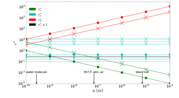
|
| Figure 9: Time scales of Brownian motion normalized by the viscous diffusion time for the same combinations considered in Table 1. Dots indicate water as the suspending fluid, while crosses imply air. The size of the markers grows with the density of the particles. |
Sticking to the common theme of this section, we will now attempt to link this theory to the MRE. Our goal is to mark the onset of Brownian motion, providing a simple rule to assess whether Brownian effects can be safely neglected. We proceed as before, comparing these effects to that of other forces as the radius of the particle shrinks, since we know Brownian motion is mostly relevant at small sizes. The focus is placed on hydrodynamics, so we should compare Brownian motion to the motion caused by hydrodynamic forces. We would also like to take the buoyancy force into account.
Comparing different hydrodynamic forces is meaningful only when their characteristic times of application are the same, which is equivalent to comparing impulses. In turbulence, the natural reference is the microscopic Kolmogorov time-scale, since it determines the time scale of the relative motion between fluid and particles (when turbulence is driving the relative motion). From hydrodynamic theory, we know that the Reynolds number represents the ratio of inertial versus diffusive momentum transport rates, that is . At the Kolmogorov scales the Reynolds number is by definition of order one, so
|
|
(2.70) |
since we have by assumption that . In fact, by the same argument, we have the even stronger
|
|
(2.71) |
This will have immediate consequence in our analysis, as we will see in the following lines.
On the other hand, Brownian motion presents a full spectrum of time and length scales for all time intervals below , due to its pseudo-fractal nature, down to the ballistic regime 6, where the velocity of the particle becomes well defined as its trajectory starts to smooth out when observed at such small scales. The ballistic regime starts roughly below [39]. This kind of motion is more appropriately described in terms of statistical averages. Here we consider the mean squared displacement (MSD) or, rather, its square root as a measure of the displacement caused by Brownian motion:
|
|
(2.72) |
where
|
|
(2.73) |
That is, the ensemble average of the Euclidean norm of the displacement after a given time lapse . In this way, can be interpreted as the amplitude of the Brownian motion at the time scale . So that, instead of comparing forces, we can compare the characteristic displacements and to each other, where the latter is the characteristic displacement due to the hydrodynamic forces, still to be determined.
We expect the very small particles for which Brownian motion might be relevant to follow the background flow closely, due to their small inertia7. So their velocity is expected to be overwhelmingly dominated by this contribution. However, it is the component of the motion relative to the fluid motion that determines many interesting phenomena in particulate flows, such as preferential concentration [112] or particle collisions [30], and so we will consider this component. After multiplying it by , we will obtain an adequate measure of displacement, due to the hydrodynamic forces.
Let us consider a turbulent flow. If the flow of interest were laminar, the same reasoning applies by replacing the Kolmogorov microscales with the typical scales of the problem at hand. If the main assumptions of the MRE are met and the particles are very small, so as to make Brownian motion potentially relevant, the scaling analysis of Balachandar [19] applies and the order of magnitude of the slip velocity can be estimated as:
|
|
(2.74) |
where
|
|
(2.75) |
and is the Kolmogorov time scale, while is the magnitude of the local fluid velocity. The estimate is derived under the hypothesis that the particle is most of the time close to steady state; that is, that the drag force dwarfs the other terms in the MRE most of the time. Such situation can be expected for very small Stokes numbers (for , according to Balachandar, as we will discuss in the following section8).
The estimate above does not include the effect of buoyancy (and weight). Balachandar takes this into account separately by keeping track of the point at which the effect of gravity dominates the other forces. That is, when the settling velocity exceeds the slip velocity from equation Eq.~2.74, which happens beyond the point where the Kolmogorov acceleration (, with the turbulent energy dissipation rate) is smaller than . In order to derive our order-of-magnitude relation, it is sufficient to separately consider the steady settling velocity, , which is obtained by balancing the drag force with the submerged weight, giving
|
|
(2.76) |
Once the order of magnitude of the slip velocity has been identified, we can construct the following time-dependent distance scale
|
|
(2.77) |
which is a measure of the inertial deviation from the perfect tracer particle trajectory of a given particle. Similarly, we define .
Now, the question is, in what circumstances is the effect of Brownian motion in deviating the particles' trajectories from the fluid stream lines of an order comparable to that caused by the particles' inertia (or buoyancy force)? We claim that an answer to this question can be given in terms of the quotient (or ); that is, the ratio of contributions to the deviation from a perfect tracer particle over one Kolmogorov eddy turnover. We propose to consider that the contribution of Brownian motion may be reasonably neglected whenever
|
|
(2.78) |
The Langevin theory [345] provides the right tool to calculate . This theory models the movement of the particle as a result of Newton's second law of motion, where the forces are given by a macroscopic contribution or resistance plus a random force originated from the molecular collisions which is modelled as Gaussian white noise 9. In particular, the often-called modified Langevin equation has recently been experimentally verified [172,160] to be accurate all the way down to the ballistic regime. This version of the equation includes, apart from the steady drag, all the other terms in the MRE. From it, Clercx and Schram [75] have derived the exact expression of the MSD, which we have written as a function of the nondimensional time :
|
|
(2.79) |
where
|
|
(2.80) |
with
|
|
(2.81) |
The parameter is a small correction, relevant only for [277]. The function defined in Eq.~2.79 has two extreme regimes; those corresponding to (ballistic regime), and (diffusive regime). It is a direct calculation to check that their corresponding asymptotic relations are given by
|
|
(2.82) |
Eq.~2.79 can be used to compute . However, we would like to provide a simple rule that would serve for most situations. For that, it is enough to realize that the two asymptotic expressions Eq.~2.82 provide sufficient accuracy when used to estimate for and as the ballistic and diffusive regimes. By gluing together the two solutions at we generate the function , that approximates . Fig. 10 shows that the error made using such expression is at most of one order of magnitude, much less for the less extreme values of . Furthermore, such estimates are on the safe side, in the sense that they are upper bounds for the value of the MSD.
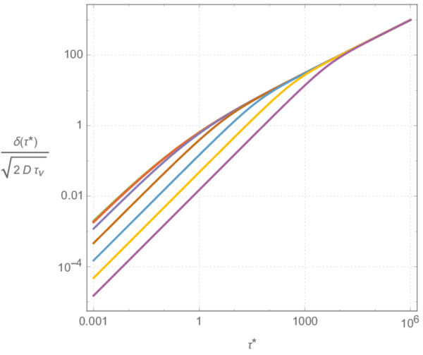
|
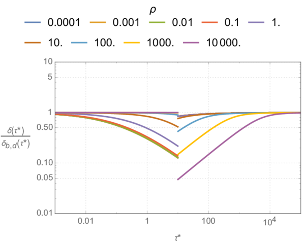
|
| Fig. 10 (a). Evolution of , normalized by the constant coefficient in Eq.2.79, as a function of the elapsed nondimensional time for a wide range of relative densities. The two extreme regimes are visible: the ballistic regime corresponds to the 1:1 slope for short times and the diffusive regime to the 2:1 slope for longer times. | Fig. 10 (b). Ratio of as calculated by Eq.2.79 over the value obtained by using its asymptotic approximations. The ballistic approximation is used for , the diffusive one being used thereon. The error is never more than one order of magnitude, and practically always on the safe side (below one). |
| Figure 10 | |
An additional observation that follows from Fig. 10 and Eq.~2.71 is that the diffusive approximation should suffice four our purposes, since its value becomes of the same order of magnitude as that given by Eq.~2.79 under the hypothesis that the movement of the particle is caused by the turbulent fluctuations of the flow and buoyancy. In these conditions, we are always to the right of in Fig. 10, and Eq.~2.78 can be expressed as (going back to the dimensional version of the MSD).
|
|
(2.83) |
where the second order-of-magnitude inequality follows from the first, after substituting Eq.~2.75, using the definition of and removing the square root; the third inequality follows after considering that an L-sized circular eddy completes a turn in a time ; the subsequent implication follows from replacing by and taking into account the fundamental hypotheses of the MRE theory (i.e., which we have taken as ); finally, the last inequality is obtained from Eq.~2.75, the fact that , the definition of and that of the so-called Schmidt number, , which is the ratio of viscous diffusion over molecular diffusion.
Now, it is clear that for the case of neutrally floating particles (), the above estimates cannot be used, because the MRE (excluding Faxén terms) predicts the particles to exactly follow the streamlines. The relative importance of Brownian motion for this case becomes unbounded due to the factor involving (see Fig. 12) and it should be compared to some other effect, perhaps higher order corrections of the hydrodynamic forces, like the Faxén corrections, or other, relevant forces. We will however leave the discussion at this point.
The settling (or raising) velocity due to the buoyancy force is systematic, just like the long-term effect of Brownian motion, so that any sufficiently long time scale is adequate to compare both effects. It is convenient to use the time it takes for diffusion to cover a distance . We have seen that for Brownian motion this time is . Therefore the condition Eq.~2.78 becomes
|
|
(2.84) |
The nondimensional number is the Péclet number associated to the settling velocity [35].
In order to put the above estimates in perspective, it is useful to examine Fig. 11, that shows the relative importance of the Brownian diffusion in front of the added effects of gravitational settling and inertial drift, for different particle sizes. The different curves correspond to different typical conditions in a variety of environments, where the ranges of parameter values (indicated with error bars) have been determined according to the typical specific energy dissipation rates and the range of values for the density corresponding to the different material combinations from Table 1, except the neutrally buoyant cases.
|
| Figure 11: Importance of diffusion relative to gravitational and inertial drift effects for different environments, as a function of the particle size. The curves correspond to the (log)-averaged values corresponding to the extremes of the typical ranges of values found in those environments, including a range of turbulent kinetic energies (human trachea: to [115] 11; free atmosphere: to [190]; ocean, mesopelagic zone: to [228]; and for the material combinations in Table 1, except for the neutrally buoyant cases. |
(1) Such phenomena can arise equally due to a decreasing particle radius, or, as well, due to a growing distance between molecules due to a drop in the average pressure.
(2) Here the Knudsen number is defined based on the mean free path given by , with the gas pressure, the gas constant and the temperature; in accordance with the kinetic theory of gases [198]. Note that it is common to encounter variations of Eq.~2.63 based on a different definition of the Knudsen number. Other, frequently used, definitions include and ; see [327].
(3) This is a more general notion of the Stokes number, where the motion is not assumed to be determined by the balance between inertia and viscous forces, as we have assumed elsewhere.
(4) We have slightly altered their notation, in that we have replaced their Brownian relaxation time () with , which includes the added mass effect; and also in calling the viscous diffusion time (instead of viscous time) and the molecular diffusion time (instead of diffusive time).
(5) Perhaps appropriately modified due to the slip boundary conditions, according to 2.62
(6) This ballistic regime should not be confused with the 'ballistic regime' that we refer to later, when speaking about the particle's response to the turbulent eddies. The notion is nonetheless somewhat analogous, in that here it refers to the particle's response to the random bombardment to the molecules. Furthermore, the relaxation time of the particle to the random impulses from Brownian motion is defined identically, since the drag law of Stokes is still valid in this regime.
(7) Here we briefly get ahead of ourselves, since this aspect will be treated in more detail in the following section. However, it can also be interpreted as a motivation example for the analysis that is done therein.
(8) Note that this argument applies to the forces induced by the turbulent fluctuations alone. The superposed Brownian fluctuations will induce additional hydrodynamic forces that we consider independently, for which the above comments must not hold.
(9) The hypothesis of the thermal noise being Gaussian (white noise) is actually only an approximation and more sophisticated coloured versions of the theory have been proposed [37].
(10)
(11) Estimated as .
2.2.6 Other effects
The list of effects reviewed in Section 2.2.1 to 2.2.5 cannot be exhaustive. In order to keep the size of our endeavour manageable, we have decided to leave some effects that are indeed important for future work. These effects include the action of common long-range inter-particle forces, such as the van der Waals and electrostatic forces; or the deviations form the Newtonian description of the fluid, for example.
Another notable omission is the analysis of the effect of boundaries in the domain, which has been ignored in this work. Certainly, the MRE is derived under the assumption of an infinite fluid domain. But, in reality, the presence of nearby boundaries often plays a fundamental role in explaining the motion of suspended particles, especially given the slow decay of the particles disturbance flow with distance as discussed in Section 2.2.4. These effects are of especial relevance to internal flows with large specific boundary surface area, such as in transport in tubes [101]; and their understanding is paramount to explain a series of phenomena in microfluidic devices; see [388] for a recent review. The characterization of the first effects of the presence of boundaries on the MRE is therefore of vital importance in order to characterize the applicability of the MRE to many industrial systems and the subject of ongoing research by the author.
With respect to particle collisions, we have commented in Section 2.2.4 that the CFD-DEM method is naturally able to take into account inter-particle collisions. However, this is only true as long as short-range inter-particle hydrodynamic forces can be neglected. Indeed, as two small particles approach each other, their Stokesian perturbations start interacting causing the particles to deviate from their non-interacting trajectory. In most cases, these interactions reduce the probability of collision between the particles with respect to their non-interacting trajectories, although they can also increase them under some circumstances [362]. The proportion of particles that collide by taking into account short-range interactions with respect to the number of particles that collide when neglecting them is called collision efficiency [169,292]. If we can find a theory that characterizes the collision efficiency in a generic turbulent flow, as a function of the flow and particle parameters, we could use it to estimate the first effects of the short-range hydrodynamic interactions on the particles and extend our analysis with them. This task is left for future work.
Another important set of effects relevant to the motion of very small particles are those related to the gradients in temperature, that produce a drift of the microscopic particles towards less energetic zones. A good review on the matter can be found in [249]. The study and characterization of these effects have also been left for future work.
2.3 Scaling analysis
The review in the previous section highlights the breadth of the applicability range of the MRE. Just like other equations that can be applied to a wide range of systems, e.g.the Navier–Stokes equations, it is interesting to study the possibility of specializing the MRE to more constrained situations. The Stokes equation is an example of such specialization of the Navier–Stokes equations. Its range of applicability is smaller (very small Reynolds number), but its higher simplicity facilitates analysis and very often its numerical solution too, making it preferable under the appropriate conditions. Similarly, the Maxey–Riley equation is often simplified in practice, typically by dropping one or more of its terms.
A necessary condition for being able to do this is that the relative weight of such terms is small compared to that of the ones retained. Scaling analysis permits estimating ranges for the characterizing dimensionless quantities for which such conditions hold. While such analyses always contain a certain (order-of-magnitude) degree of uncertainty, their precision is often sufficient and can later be compared to empirical evidence to reinforce them and refine them if necessary.
In this section we apply an order-of-magnitude analysis to study these questions and quantify the relative importance of the different terms.
2.3.1 Analysis of a simplified MRE
In this section we mainly draw from [79,19,211]. We strived to unify the most relevant parts of these works, which had not been done by the most recent author. Our results are very similar but still in some parts different to that of these authors.
Let us consider a simplified version of the MRE in which, for the moment, we neglect the Faxén corrections and the buoyancy terms. For this case Eq.~2.2 reveals that the Stokes number controls, at its limits (i.e. and ), the relative importance of the viscous terms with respect to the pressure terms. Specifically, making large enough (while leaving and fixed), for example, by making the size of the particles very big, will make the first two terms negligible and the acceleration of the particle will be completely dictated by the drag and the history terms. Conversely, if tends to (e.g.by making small), only the first two terms contribute, while the drag force becomes negligible. Note however that such limit can never be reached without destroying the validity of the equation, since it is valid in the limit of vanishing and that for to characterize the flow around the particle, it is necessary that . Moreover, this form of the equation does not immediately show that the viscous terms vanish for , as this case corresponds to a fluid point-particle (that will therefore lead to a vanishing relative velocity with respect to the fluid).
We have seen that by inspection of the nondimensional coefficients of the varying terms in the ODE one can have an idea of the asymptotic behaviour of the ODE. However, it would be naive to directly compare their magnitude in order to assess the relative importance of the different terms. The reason is of course that there is no guarantee that the dependent variables they multiply are all of a similar order. This is exactly the issue that can be addressed by order-one scaling (-scaling) [197]. The method consists in precisely making sure that the dependent variables range the interval between zero and a quantity of order one and thus their coefficients directly reflect their relative weight. The method is iterative, and we will skip the details, although we will include the nondimensionalized equation and justify the order-one boundedness of each term. While the notion of is not completely rigorous, it should be understood to mean that the referred value lies well within an order of magnitude of one. This notion, while imprecise mathematically, should be useful from an engineering point of view. It should therefore be viewed a method to systematically produce postulates about the size of the error one is making, to be refined by experience and further analysis.
Let us therefore consider an unspecified background flow that nonetheless can be regarded as an oscillatory, periodic flow. A useful mental image could be a sinusoidally varying signal (for each spatial component) or a single eddy inside which the particle is submerged. Let us consider that the period of this flow is given by and that its velocity's magnitude is bounded by . We additionally consider that its wavelength is given by (i.e.the diameter of the eddy). Our goal is to characterize the reaction of the particle to a generic fluid perturbation. We will consider that sufficient time has passed so that all information about the initial conditions (when the particle was first introduced in the flow) has been forgotten. We consider the evolution of the particle during one period, and, thus, the temporal domain is given by . Let us write down the appropriately simplified version of equation Eq.~2.1:
|
|
(2.85) |
The lower limit of the integral in the Basset term has been set to minus infinity to account for the fact that initial conditions have been forgotten. We now nondimensionalize the equation by introducing the scalars , , , and such that
|
|
(2.86) |
where we require that , and normalize their associated variable, in such a way that its characteristic value is one. Applying these relations to Eq.~2.85, dividing through by the coefficient of and, again for notational simplicity, dropping the asterisks to denote nondimensional variables we obtain
|
|
(2.87) |
Note that since all the dimensionless variables are now of order one (assuming that none is exactly null), the constant coefficients of the different terms can be interpreted as their characteristic sizes. Since the drag force is (almost) always retained, we will compare the importance of the other effects with respect to it, by evaluating the following quotients.
|
|
(2.88) |
where we have used the notation and so on for the magnitudes of the different forces.
At this point, it is convenient to distinguish between two regimes: that for which , which we may call the tracer-particle regime and that for which , or the ballistic regime.
Tracer-particle regime
In the tracer-particle regime the particle relaxation time is smaller than the turnaround time of the smallest eddies in the fluid by definition, and so its velocity has time to become similar to that of the fluid, except perhaps for values of very close to one. This allows us to consider that . Evidence supporting this scaling can be found in [392].
We now introduce a simple model to estimate the magnitude of the slip velocity . Let us consider a particle moving within an eddy of size . Since, according to Eq.~2.88, in this regime the drag force is never dominated by the history force or the added-mass force, its magnitude must balance that of the rest of terms in the MRE. Approximating the particle velocity to that of the fluid velocity, the drag force must balance inertia and the force due to the unperturbed flow. That is
|
|
(2.89) |
where the LHS is the centripetal force plus the force as would be applied to the displaced volume in an unperturbed fluid (minus its centrifugal force). Note that this agrees with the expression given by Balachandar [19], using a different argument. Furthermore
|
|
(2.90) |
with these estimates we can develop Eq.~2.88 into
|
|
(2.91) |
It is interesting to compare the expression for the importance of the history force to the estimate proposed in [90], where the following estimate is given in the context of direct numerical simulation of turbulence
|
|
(2.92) |
where a good fit to their numerical data was found for . It is easy to see that, for the present low inertia case, our estimations are basically equivalent, since (excluding the case of nearly neutrally buoyant particles, which was not addressed in [90])
|
|
(2.93) |
where we have used the fact that for non-nearly buoyant particles , that and that the characteristic scales of the flow are given by the Kolmogorov microscales. The negative sign in the RHS indicates that this force tends to diminish the slip velocity. Note that the RHS of Eq.~2.93 is equivalent to that of Eq.~2.92 to first order in , where the role of in Eq.~2.92 is played by the order-one quantity ).
The condition Eq.~2.9, i.e. that the particles must be substantially smaller than the smallest fluid scales, strongly limits the importance of the added mass term and, to a lesser extent, the history term. To see this, let us use Kolmogorov's theory of turbulence, to estimate
|
|
(2.94) |
However, if the unsteady force is to be important, the characteristic time has to be small enough. Indeed, will be important (with the usual one percent relative magnitude threshold) if
|
|
(2.95) |
Note that only by relaxing the condition of small particle radius this force can (just about) reach the region in which it is important. For instance, by only requiring that . But since it has been shown that the validity of the MRE can be extended beyond (see Section 2.3.2), it is still of interest to take these forces into account.
Similarly, the analogous condition to Eq.~2.95 for the history force in this regime is
|
|
(2.96) |
Note that here the history force will be just about important with the strict interpretation () of Eq.~2.94 and will have a region of importance spanning two orders of magnitude if the more permissive condition is used.
Ballistic regime
For , the particles are too slow to react to the smallest fluid scales and thus here Eq.~2.89 is no longer a good approximation. We use the same reasoning as in [19]. By considering the limit of expression Eq.~2.89 approaches one, one obtains
|
|
(2.97) |
Now, considering that this expression is valid down to , we argue that by taking larger values of one does not increase the slip velocity any further (in order-of-magnitude terms), since the velocities of the particle are already largely uncorrelated. On the other hand, should not increase to much larger values than , since its movement is caused by the surrounding fluid in the absence of external forces. Again, we find empirical evidence for this in [392]. The estimates for the derivatives are now
|
|
(2.98) |
with these estimates for the slip velocity we obtain
|
|
(2.99) |
Note that the relative weight of the history force is now dependent on the Stokes number. For large Stokes numbers, the non-dissipative forces have larger relative weights, diminishing the importance of the history force, that is more heavily penalized for large values of than in Eq.~2.91. This is not captured by Eq.~2.92, leading to an over-prediction of the importance of the history force as which clearly shows in Figure 4 (b) in [90].
With regards to the limitations imposed by Eq.~2.9, the analogous pairs of conditions to Eq.~2.95 and Eq.~2.96 read
|
|
(2.100) |
which are essentially the same conditions as in the tracer-particle case with the factor , whose behaviour is shown in Fig. 12.This quantity is always greater than one and of order one in most of the domain. It is only close to the neutrally buoyant case () that its value explodes asymptotically. But of course in this case the drag force ceases to be a dominant force, since neutrally buoyant particles tend to behave as perfect tracers. In this case one may normalize these forces by instead, which gives
|
|
(2.101) |
|
| Figure 12: Behaviour of the factor . |
Nearly neutrally buoyant particles
In this regime, the force that the fluid particles feel is very close to that would be felt by a fluid particle. This means that the most dominant force, by definition, is . The estimates for the slip velocity given for the tracer-particle regime are still valid here, and thus the relative magnitudes between the different forces are preserved. It is nonetheless interesting to present their magnitudes this time normalized by . The results are
|
|
(2.102) |
where we have used and in the two last estimates. On the other hand, cannot be reached for , since this leads to the violation of Eq.~2.94, and the MRE is not applicable.
2.3.2 Importance of the Faxén terms
The Faxén corrections arise as approximations of volume and surface integrals of the fluid field over the particle [238,222,53]. These terms are almost universally neglected, although there are very few number of studies to discuss the validity of such assumptions, highlighting their relevance when the particle radius approaches the size of the smallest scales in the fluid [53]. Let us analyse their importance, through scaling arguments.
Whenever the slip velocity is substantial, compared to the velocity of the fluid, their importance is necessarily small within the range of applicability of the MRE, since they are proportional to the radius of the particle squared and thus
|
|
(2.103) |
which means they are small corrections to the terms they accompany. We thus concentrate on the situations where the slip velocity is expected to be a small fraction of the fluid velocity, such as when is significantly smaller than one. Then, using the estimate from Eq.~2.89 instead one finds
|
|
(2.104) |
where we have used the fact that for all the Faxén terms, that and that the Reynolds number of the Kolmogorov scales is of order one. Note that this result is remarkable: in this regime the Faxén terms are important regardless of how small the particle is, compared to the drag force and thus cannot be neglected unless the particle is substantially more dense than the fluid.
However, this estimate cannot be universally valid, since for close to one, the Faxén corrections become dominant in the drag force term and so the assumptions made in the derivation of Eq.~2.89 are incorrect. This means that a different route must be taken to assess the relative importance of these terms. We follow the same procedure as in [171], considering an asymptotic expression with 1, where represents the Taylor microscale, as the small parameter. The procedure consists in considering the particle velocity as a perturbed version of the fluid velocity, that is
|
|
(2.105) |
where is an unknown function and is an unknown exponent, both to be determined. Note that in the present discussion it is guaranteed that . Neglecting the added mass and history terms (since those are uniformly smaller than the drag force for small Stokes numbers and , see Eq.~2.91) in Eq.~2.1 and dividing through by , one obtains the following equation
|
|
(2.106) |
Substituting Eq.~2.105 into Eq.~2.106 yields
|
|
(2.107) |
where we have used the relation . Let us compare the orders of magnitude of the various terms.
|
|
(2.108) |
where represents the characteristic module of . Note that the fourth term is of a greater order than the first, due to the assumption of nearly-neutrally buoyant particles, and the third one, for the same reason (reinforced by the assumed smallness of the Stokes number). Furthermore, the fifth term is at least significantly greater than the second one due to the smallness of the Stokes number. This means that the fourth and fifth terms must be of the same order to fulfil Eq.~2.107, which provides an estimate for the first-order correction, since it must hold that
|
|
(2.109) |
which means that and . Note that this result is not consistent (although of the same order) as the one reported in [171], where the six in the denominator is replaced by a ten. Note that nonetheless, in this work it is stated that "the first-order terms originate from Faxén corrections to the Stokes drag", which would be consistent with the one-sixth factor that we have obtained here. In summary, the Faxén corrections become the dominant correction to the particles' velocities for nearly neutrally-buoyant particles, and this correction is proportional to the particle radius squared. Based on the asymptotic reasoning above Homann and Bee [171] give the following estimate for the averaged effect of this term, based on the assumption of isotropic turbulence
|
|
(2.110) |
where the would be according to [171]. This implies that this effect is small in the range of validity of the MRE. Indeed these authors study the importance of the Faxén corrections for finite-radii neutrally-buoyant particles and confirm that this effect only becomes significant outside this range. They conclude that tracer-like behaviour is prevalent for radii smaller than and that the effect of the growing radii is well described by the Faxén corrections up until , point at which inertial effects start to become important (note that at this point we are well outside the theoretical range of applicability of the MRE).
(1) For the sake of clarity, let us mention that these authors considered as the small parameter.
2.4 Summary
In this chapter we have applied scaling analysis to the Maxey–Riley equation and to a selection of the hypotheses that support its validity. Our goal was to move closer to a complete characterization of the range of validity of this equation; to be useful as a tool for the assessment of the reliability of the numerical simulations based on it. We are guided by the idea that a physical model equation, such as the MRE, should be tightly attached to its domain of applicability, which is in fact also part of the model. We envision that in the future all the information that is currently dispersedly stored in distributed support (i,e. a combination of human brains and remarks in the literature), will be much more connected and centralized and encoded in a non-ambiguous way. According to such a paradigm, one should be able to program more sophisticated algorithms that automatically analyse the validity of the models used, and that generate estimates of the error according to a variety of measures.
If we model the range of applicability of the MRE as a manifold formed by the combinations of possible values that the relevant non-dimensional quantities may attain (as a function of the desired level of accuracy), our objective is to characterize this manifold by identifying parts of its unknown boundary.
Our analysis has produced a number of conditions on a set of dimensionless quantities that characterize the problem of the motion of a single particle in a Newtonian fluid. A first subset of these parameters resulted from the analysis of the dimensionless parameters that parametrize the equation itself. These are , and ( was not explored). A second set of parameters were taken into account explicitly in the derivation of the MRE [238], where it is required that they are small. This is the case of . The rest of the parameters must be introduced from outside the theoretical background of the MRE to analyse its range of validity. Such are , , related to the inertial effects; , related to the nonsphericity; and , and related to the limits of the continuum description of the flow, for very small particles. Finally, we also tackled the problem of characterizing the first effects of the presence of neighbouring particles in the flow. Within our limited theoretical framework (uniform suspensions or infinite, isotropic turbulence with heavy particles), the relevant nondimensional quantities have been identified to be and . The main results are summarized in Tables 2 to 5.
| Dimensionless parameter | Applicability condition | Error measure and growth rate | Associated effect |
| Onset of inertial effects on drag force | |||
| Lift force due to shear | |||
| Lift due to the Magnus effect | |||
| 1 | Effect of nonsphericity | ||
| Breakdown of no-slip B.C. for gases | |||
| Brownian effects vs inertial drift for liquids | |||
| Brownian effects vs gravitational settling |
| Dimensionless parameter | Applicability condition | Error measure and growth rate | Associated effect |
| see Eq.~2.39 and equations leading to Fig. 7a | Onset of collective effects in settling | ||
| see Eqs.~2.55 and 2.59 | Collisions become important in the macroscopic flow |
| Tracer-particle regime | ||||
| Ballistic regime | ||||
| Nearly-neutrally buoyant particles |
| Tracer-particle regime | Ballistic regime (non-neutrally buoyant) | Nearly-neutrally buoyant particles |
(1) The rate depends on the particular shape of the particle; see Eq.~2.29.
3 The numerical solution of the Maxey–Riley equation
3.1 Introduction
Particle-laden flow simulations typically involve a multitude of particles, even for highly disperse regimes. And while it is sometimes possible to form representative ensembles by instead considering only a small fraction of the actual particles [318], their total number must still be large enough to ensure statistical significance, often a demanding requirement. For methods that track the evolution of each individual particle, as in Euler-Lagrange methods, this translates into solving the single-particle equation of motion (i.e., the MRE) a correspondingly large number of times. As mentioned earlier, the associated computational costs can quickly become cumbersome and thus efficiency becomes of great concern.
Without the history term, the MRE is an ordinary differential equation, whose solution is well known to be regular for a sufficiently smooth background fields [124]. Its numerical solution can be achieved by standard integration schemes like the Runge–Kutta methods [215] or the Adams-Bashforth schemes [330] in a reasonably efficient way. Both explicit and implicit methods can be used. Explicit schemes are conditionally stable and require small enough time steps. This requirement can become quite severe, especially when unsteady effects are included (added mass and history force). This is why many implementations use implicit strategies instead [221].
In the context of (soft-sphere) discrete element methods, explicit schemes are nonetheless the preferred option in the vast majority of implementations. This is because explicit algorithms are already the most common choice for regular, dry DEM algorithms. In such case, the contact forces enter the RHS of the MRE simply as additional external forces. These forces have a very small characteristic duration and often pose an even stricter bound on the maximum allowable time step than any of the hydrodynamic forces.
Other, hybrid options are also possible. For instance, implicit scheme for the MRE can be combined with an explicit treatment of the contact forces to improve stability. Fully implicit schemes, treating both the contact and the fluid interaction implicitly are rare. For a comparative review of various integration schemes for fluid-coupled DEM, see [348].
In summary, whether explicit or implicit, relatively standard and efficient methods have been shown to work with the MRE without the history force term.
On the other hand, the presence of the history term turns the MRE into an integro-differential equation (in fact, to a fractional differential equation, see Section 3.2.1) with qualitatively different mathematical properties (in particular, the dependence of the force on the whole trajectory of the particle) 1. Furthermore, its presence complicates the numerical solution of the MRE, due to the necessity to calculate an (improper) integral over the whole past history of the particle, at every time step. Straightforward extensions of standard methods either fail or become extremely inefficient here.
Perhaps for this reason, the history term has been routinely neglected (see, for example, [212,286,241,235]), although clearly not always on a solid physical basis. For instance, for the numerical study of bubbly turbulent water flow, its effect was neglected a priori in [242], without explicitly commenting on it. However, the range of parameters in the examples examined therein do not justify this, according to Table 4 and values and that used in that work. Notwithstanding this, awareness of this issue is growing within the scientific community as a number of (mostly numerical) studies provide new evidence of the importance of including this force in a variety of contexts [155,266,90,254].
This chapter is concerned with the discretization and numerical solution of the MRE. We focus on the numerical treatment of the history force term, reviewing the state of the art and making several contributions to the subject. We present a complete algorithm to take advantage of the previous developments and we test its accuracy and efficiency in a sequence of tests of increasing level of complexity. We conclude that the proposed algorithm permits the inclusion of the history force in large-scale particle-laden flow simulations at an acceptable cost.
(1) It is perhaps appropriate to mention at this point the recent proof, given by Farazmand and Haller [124], of local existence, uniqueness and regularity of (weak) solutions of the MRE (including the history term) under quite general conditions. In particular, the proof requires the fluid velocity field to be at least four times continuously differentiable in space and time over the whole trajectory of the particle and that its partial derivatives (including mixed partials) are Lipschitz continuous and uniformly bounded up to order three.
3.2 Overview of approaches for the treatment of the Boussinesq–Basset term
In this section, we briefly review the state of the art in the numerical treatment of the history term, introducing the challenges it poses and how researchers currently go about overcoming them. For more information, see the recent review by Moreno-Casas and Bombardelli [254]. Our review will also serve to introduce the methods and notations that are used in this work to treat the history term, some of which have been modified or further developed. This is the subject of the subsequent sections.
The Boussinesq–Basset force term has the form of the derivative of an integral, as presented in Eq.~2.1. In considering the finite-difference discretization of the MRE, the derivative becomes a finite difference and thus one is faced with the question of how to evaluate the integral at a given discrete time. Let us start by recalling its exact form (ignoring the coefficient ):
|
|
(3.1) |
which can be rewritten as
|
|
(3.2) |
where defines the Boussinesq–Basset kernel function and a differentiable vector field (assuming the unknowns to be smooth enough). Thus, the integral above can be understood as the convolution of with the kernel . Note that, with this notation, we have .
It is also possible to consider a different form of the Boussinesq–Basset integral, where the derivative moves under the integral sign; see Appendix C. Specifically
|
|
(3.3) |
where the alternative form is on the right-hand side. The latter was precisely the one used in [353], though its second term vanished because the initial time was taken as . Nonetheless, the same method can be applied to both situations; it is only necessary to correctly identify the field that must be considered: either , or its derivative 1. As pointed out in [89], the first form is very convenient because it eliminates the need to compute either any additional derivatives or the second term in Eq.~3.3. It is for this reason that we have also adopted this form in this work.
A naive approach would be to use a classical quadrature scheme (e.g.Newton-Cotes formula) to express the integral in terms of a finite number of discrete values of the unknowns. An initial difficulty is encountered when trying to evaluate the integrand at the current time, since the integrand is actually not defined at that point. Still, semi-open interval quadrature formulae can be found to overcome this difficulty. Daitche [89] refers to the semi-open Newton–Cotes scheme [129] in this regard. Two alternatives are mentioned in [40]: the Euler-Maclaurin formula [129] and a method that had been apparently proposed by L.M. Brush et al. in 1964. The latter consists in applying the following approximation
|
|
(3.4) |
where is evaluated in some point in and a standard quadrature rule is then to be applied to the (now proper) integral on the RHS. The first two methods where shown to yield errors that scale like . In Section 3.5.1 we implement Brush's method, which also shows the same order of accuracy. Such low-order methods lead to excessively small time steps and, we will be interested in finding higher-order quadrature schemes to replace them. First, however, we introduce the concept of a fractional derivative, a generalized definition that allows us to define the history term in an elegant way.
(1) Such derivative would involve a finite difference representation of the unknowns and the fluid field values under the integral sign, leading to a stencil involving the linear combination of quadratures at different points in time.
3.2.1 Fractional derivative approach
The theory of fractional derivatives generalizes the classical derivatives and anti-derivatives (indefinite integration) of integer order, by letting this order take arbitrary real values. There exist a rather large number of alternative ways in which this generalization has been realized, leading to a profusion of derivative definitions that has recently been summarized in an extensive survey by de Oliveira and Tenreiro [94]. Letting be a function defined in an interval , its Riemann-Liouville left-sided derivative is defined, for all , as
|
|
(3.5) |
where represents the derivative order and is Euler's Gamma function and the subindex indicates that the derivative is defined for (Sometimes the alternative notation is used).
A different definition for the fractional derivative is given by the Grünwald–Letnikov derivative. This derivative is obtained by generalizing the usual finite difference formulas and taking the limit to vanishingly small step size. The definition (left-sided version) reads
|
|
(3.6) |
where .
The following lemma relates both definitions [279, p. 76]:
Lemma 1: Let be continuous and its first order derivative be integrable in . Then, for every both the Riemann-Liouville and the Grünwald–Letnikov derivatives of exist and are equal.
The observation that the Boussinesq–Basset force can be understood as a fractional time derivative (times a constant), was apparently first made by Tatom [338]. Specifically, this term is proportional to the Riemann–Liouville fractional derivative of order of the slip velocity (plus the Faxén corrections); that is
|
|
(3.7) |
since , where the derivative operates component-wise.
The Grünwald–Letnikov representation of the derivative suggests an approximation method to compute : pick a small and compute the resulting finite sum. And, indeed, under the assumptions of the above lemma, this approximation may also be used to calculate the Boussinesq–Basset force. This possibility was, to the best of our knowledge, first explored by Bombardelli et al. [40], see also [148] (although Tatom already acknowledges the possibility of using the Grünwald–Letnikov representation for numerical computation). These authors tested the summation method (hereafter referred to as the GL method) against a standard method (i.e.the Euler-Mclaurin summation formula, mentioned in the introduction of this section) to deal with the kernel singularity at the time. They found that the method was more efficient, achieving first order scaling of the error, as opposed to the order one half achieved with the standard method. It was not long, however, until new techniques appeared ([353], followed by [89]), achieving second and higher accuracies and somewhat overshadowing this more exotic method. In [353], the first order accuracy obtained by Bombardelli is referred as a motivation to look for alternative, higher order methods. Furthermore, in the recent review of Moreno-Casas and Bombardelli [254], it is concluded:
For the accuracy in the computation of the standard term, the intrinsic difference between all three methods is the order of accuracy of each approximation. Whereas the approach of Bombardelli et al. [40] leads to a first-order solution in the computation, the method by van Hinsberg et al. [353] leads to a second-order solution, and the Daitche approach [89] sets grounds to obtain higher order solutions (second-order and higher).
While their remark captures the behaviour of the algorithms as were presented in the cited works, we think it is excessive to talk about an intrinsic difference between the methods. In Section 3.5.1 we will argue that Bombardelli's approach can be modified to achieve higher order accuracies. Similarly, we will view the method of van Hinsberg et al., not as an alternative to the other methods, but actually as an evolved version of them. This point is addressed in the Section 3.3.
3.2.2 Hybrid polynomial interpolation/analytic approach
The idea of using a polynomial interpolation to approximate only the nonsingular part of the integrand ( in Eq.~3.2) was introduced by van Hinsberg et al. [353], who used linear polynomials and obtained a first-order accurate method. That is, they showed the quadrature error to scale with ; being the distance between successive quadrature points, assumed to be equal to the time step. This performance beat standard methods (for example, the second order Euler-McLaurin formula, of order one half) but also the fractional derivative approach used by Bombardelli (first order accurate). The method consists of the following steps:
- Subdivide the integration domain, in subintervals , with . The boundaries of these intervals are all the scheme's intermediate time integration points up to the present time, .
- Interpolate in the interior of each interval with a linear polynomial.
- Replace by its interpolated approximation back into the integral and find its primitive (it has a simple analytical formula).
- Reorder the resulting expression as a weighed sum of the values . The result is the discretized version of the Boussinesq–Basset history force,
- Plug the expression into a suitable time integration scheme. The resulting algorithm expresses the force at every time step as a function of the unknowns at all the past (and current) time steps.
The method was recently extended (and slightly generalized to allow nonzero initial relative velocities) to third and fourth order by Daitche [89]. We describe his approach in Section 3.3, as it is part of our proposed algorithm.
3.2.3 Comparing the accuracies of the different quadrature methods
Let us take look at the performance of the different quadrature methods in approximating an integral with known analytical closed form. As a test function we choose . We are looking to approximate the value
|
|
(3.8) |
where the represent Anger functions [267]. Fig. 13 shows the performance of different methods for different values of the quadrature time-step, . The sequence of is formed by doubling each consecutive value. The error is defined as
|
|
(3.9) |
where corresponds to the numerical approximation for the quadrature time step and has been chosen to be a subset of all the discrete times in which the interval is subdivided. Specifically, is contains a number of equidistant points equal to the minimum between 3.2x101 and the total number of points in each case (so as to save computational time). The point was included in all cases. Numerical experiments show that the number of points considered does not significantly modify the plot. Therefore in subsequent experiments only eight time points will be considered.
Figure 13 is very similar to the one presented in [89] for the same test. the main difference is the inclusion of the fractional derivative method, of order 1. As expected, the numerical behaviour of the error scales as . The worst performance corresponds to the Newton–Cotes method (trapezoidal rule), with the modification proposed by Brush that we described at the end of Section 3.2.
|
| Figure 13: Scaling of the global error of the different methods for the test-case |
3.2.4 Addressing memory requirements: window methods
Even though the methods discussed above achieve considerable improvements in accuracy (therefore allowing for larger time steps) with respect to standard techniques, their memory requirements are still large. Especially for systems with many particles, the necessity of keeping track of the complete history of each of them is highly demanding. Let us consider a system with particles. If we assume a time step of 1x10⁻² (i.e., value chosen for the accuracy tests in [89]) and a simulation duration of 1x101, the necessity of storing one vector per time step and particle leads to a total 1x10⁸ vectors or, roughly, about 1 G in memory (assuming a vector takes up bytes) by the end of the simulation!. Furthermore, the data contained in these vectors must be continually accessed, inside the innermost loop of the algorithm, for each particle, at every time step. Obviously, this tends to dramatically slow down, making it clear why this force has so often been neglected in the past. Window methods deal with this problem directly.
Window methods make use of the decaying influence that the past has on the advancing present value of the history force to avoid having to store the complete history of the particles. The simplest approach consists in neglecting the contribution of the particle's history that is older than some cut-off time , where is the current time. One refers to as the window time, because only the history within the window is taken into account. That is, one considers
|
|
(3.10) |
which is equivalent to
|
|
(3.11) |
The integral on the right-hand side of Eq.~3.10 is termed the window contribution, while the integral on the left-hand side of Eq.~3.11 is the tail contribution. The idea is to employ some method like, for example, any of the ones mentioned above to calculate the window contribution and to simply neglect the rest, thereby saving all the associated memory space (and avoiding the corresponding computations). As such, this method corresponds to what is known as the window method in literature, following its introduction by Dorgan and Loth [108]. These researchers applied it to the case of finite particle Reynolds numbers, taking advantage of the faster decaying nature of the history force kernel in this case 1, see for instance [223]. Here we apply the term window method generically to any method that records only a limited part of the particles' most recent history. The main weakness of the original window method is its poor accuracy, precisely due to the slow decay of the convolution kernel in time (as the inverse of the square root for the Basset kernel); because one is thus forced to increase significantly to keep the tail truncation error low, at the cost of sacrificing potential memory savings.
A much more accurate window method was proposed by van Hinsberg et al. [353] (henceforth referred to as MAE for Method of Approximation by Exponentials). In it, the tail contribution is not neglected but rather approximated. Specifically, while in the window region the kernel is kept exactly equal to the Basset kernel, in the tail region it is only approximated by a different, special kernel. The advantage of this special kernel is that it leads to a recursive expression of the evolution of the Basset integral in time. That is, the evolution of the integral from one time step to the next can be expressed in terms of its value in the previous time step plus a contribution that depends only on the recent history. Despite its relatively recent development, the method has already found application in the study of particle-laden turbulence; see [72], [188] and [352].
(1) The exact formulation includes an algorithm to approximately determine so as to minimize the truncation error. But since we would like to have as small as possible, we cannot in general apply it without running into a conflict
3.3 Improvements on the MAE
Let us review the MAE in sufficient detail. The goal is to define an algorithm to compute the integral in Eq.~3.2 approximately. We begin by replacing the Boussinesq–Basset Kernel by the modified kernel , defined by
|
|
(3.12) |
where as before and the tail kernel is defined by
|
|
(3.13) |
with
|
|
(3.14) |
and
|
|
(3.15) |
Which introduces free parametric constants, and . In other words: we replace the Basset kernel by a linear combination of exponentials at the tail. As for the form of the functions, van Hinsberg et al. reason as follows: Let us consider the unknown parameters to be a set of points that belong to the interval . Let us then impose the condition that the graph of each be tangent to that of at the these points . This condition looks to align the exponentials with the reference curve, so that a much smaller set of good candidate exponential approximants is considered. Precisely setting and as in Eq.~3.15 fulfils this purpose. The hope is that this choice will later facilitate the determination of the sets of parameters and .
Now, instead of Eq.~3.10, one has
|
|
(3.16) |
where we assume . Thus, the whole integral becomes the sum two terms: the first term on the right hand side, , is the window contribution, which can be calculated with any of the aforementioned methods (In particular, Hinsberg et al. employed the method explained in Section 3.2). The second term, , is the tail contribution and is calculated as explained below.
The use of exponentials to approximate the tail of the kernel becomes the key that permits a recursive calculation of the tail integral, which leads to a radical decrease in memory requirements. Let us now show this recursive property of the tail kernel. It is enough to consider a single exponential term:
|
|
(3.17) |
where we have introduced the auxiliary function to show the recursive property. Therefore
|
|
(3.18) |
where
|
|
(3.19) |
and where a suitable temporal discretization of must be provided. Note how only recent values of the integrand are involved in the calculation of ; all the information regarding older values is extracted, in Eq.~3.19, by referring to the old value of the integral itself.
Of course, it is still left to define parameters and . Let us for this purpose consider the error associated with the approximation of by , which we would like to have as small as possible:
|
|
(3.20) |
where is the approximate history force, obtained using in place of and denotes the usual vector modulus. Note that we have employed the RHS form of Eq.~3.3 also for the kernel . This is possible, given the regularity of , see Appendix C. Furthermore, it is straightforward to generalize the bound given in [353], see Appendix D:
|
|
(3.21) |
where is obtained from by replacing the with their rescaled analogues, and and is defined by
|
|
(3.22) |
In fact, these authors considered only the limit , at which the first term in the parenthesis in Eq.~3.21 vanishes. Their interest was therefore to find a good approximation for long simulation times. Indeed, by taking this limit in Eq.~3.21, we recover the bound derived by [353]:
|
|
(3.23) |
Now, an important observation to be made at this point is that the bound in Eq.~3.23 is also a bound for all values . This means it is legitimate to take it as a reference for real, finite-time simulations. Like Hinsberg et al. we now concentrate in this bound, with the idea of minimizing it.
Hinsberg et al. point out that the minimization of the quantity between parenthesis on the right hand side of the inequality Eq.~3.22 is not amenable to the standard Newton–Raphson algorithm. They propose the following substitute objective function, which is differentiable with respect to the unknown parameters and :
|
|
(3.24) |
The first step in the optimization procedure proposed by the same researchers is to make a reasonable choice for and then to calculate the optimal parameters by applying Newton–Raphson's algorithm. About the choice of , the only indication that is given is to make the choice of so that they cover a great range and they become closer as they become smaller. A single set of values was provided in [353], specifically, the 10-member set , for which the corresponding Newton–Raphson-averaged values were also provided.
The method has proved remarkably effective in reducing the computational cost of the simulations [353,254]. Nonetheless, the method still leaves room for improvement. In particular, the following issues are not properly addressed within it:
- the possibility of having a nonzero initial relative velocity, which is not taken into account
- the unexplored possibility of using a different time step for the quadrature
- the choice of the , which is not well defined (it relies on guessing)
Point a) we have briefly touched upon, showing that the method's bound is still applicable in this case. Nonetheless, we do not pursue here an adaptable method which should include the dependence in time of the kernel's free parameters. Item b) will be addressed in Section 3.3.1, where it is discussed in relation to the Discrete Element Method. Item c) is the objective of Section 3.3.2.
3.3.1 Introduction of quadrature substepping
A well-known feature of the soft-sphere DEM is its requirement of very fine temporal discretizations. The reason is the simultaneous time resolution of phenomena whose characteristic time scales have different orders of magnitude, which is inherent to the approach. Indeed, the time discretization of the small time scales (dynamics during contact) determines the minimum resolution of the whole simulation, whose total duration is of a much larger scale. The inevitable result is a very large total number of time steps.
While it is often possible to artificially soften the contact model to increase the smallest time scales without significantly altering the macroscopic response [95], this procedure can only be justified up to a certain point and is fundamentally limited by the necessity to stop the particles going through each other. The immediate consequence is that often the time resolution is excessively great for the description of bigger time scales like, for example, the acceleration of the particle due to the hydrodynamic forces.
Similarly, the time step associated with the quadrature of the Boussinesq–Basset integral might be unnecessarily small for the required precision if it is made equal to the overall integration time step. Accordingly, in this section we make the necessary modifications to the methods proposed by Daitche and van Hinsberg et al. to develop a more general method allowing for larger quadrature steps, while still falling back to the standard version when the quadrature step is made equal to the general time step. We refer to this technique as quadrature sub-stepping. Daitche refers to the numerical computation of the Boussinesq–Basset term for a given time as the quadrature method, while saving the term integration for the numerical time-integration of the equation of motion. In the same spirit, we speak of quadratureevery time we refer to the calculation of the Boussinesq–Basset integral (e.g.quadrature time step) while the alternative context can be assumed otherwise (e.g., time step of the integration scheme).
Up to this point, the time discretization has been defined (both time steps of the scheme and quadrature points) solely by the sequence of discrete times and the time step, . Now it is necessary to consider an additional sequence and a second time step . In our notation, the finer time discretization, corresponding to the overall scheme, is defined by and ; while and define the coarser discretization used for the quadrature.
In order to make both discretizations conformal, we consider the most recent quadrature step to have a variable length, equal to , such that and , with a positive integer; while keeping the length of the remaining steps, , fixed. At the initial stages of the simulation, one new evaluation of , is added to the growing list every time a whole quadrature step is completed (i.e.when becomes equal to one). Once the simulated time has increased by , the integrand list stops growing and every new evaluation added to it is compensated by removing the oldest one at the end of every quadrature step. The situation is represented in Fig. 14. Note that time-step numbering changes in time according to the following formulas
|
|
(3.25) |
Adapting the window contribution formulas
While any of the methods reviewed in Section 3.2 could be used, we will focus on the hybrid polynomial interpolation/analytic approach. We will first describe it in detail, closely following [89]. We will then proceed to generalize the method.
By following the steps outlined in Section 3.2.2 using Lagrange polynomials of a given order, one obtains particular versions of the method. The generic quadrature formula for any order reads, after conveniently reordering and grouping the different terms (see [89])
|
|
(3.26) |
where the coefficients are constants. The use of an extra index indicating the polynomial order of the interpolation is avoided. Instead, Daitche replaces with (first order), with (second order) or with (third order) when particularizing. We will restrict our attention to the first and the second-order versions of the method. The formulas for the and coefficients are
|
|
(3.27) |
|
|
(3.28) |
In our proposed quadrature sub-stepping scheme, the most recent quadrature step is shorter than the rest, its length being , according to Eq.~3.25. The formulas in Eq.~3.27 and Eq.~3.28 are however only valid for the special case , so they need to be modified. The length change of the most recent step has two effects. First, it affects the definition of the Lagrange polynomials that interpolate at the most recent point, . Second, it changes the formula for itself, appearing in the argument of the kernel in every integral. A quite detailed derivation of the formulas is included in Appendix B, where an inconsistency found in Daitche's paper (though not affecting the correctness of the order-specific formulas Eq.~3.27 and Eq.~3.28) is discussed and fixed. The generalized formula for is
|
|
(3.29) |
and the one for reads
|
|
(3.30) |
Adapting the tail contribution formulas
In addition to modifying the window contribution formulas, the introduction of quadrature sub-stepping also requires adapting the tail contribution formulas of the MAE. From Eq.~3.3, we have
|
|
(3.31) |
while
|
|
(3.32) |
Let us see how this method generalizes to include sub-steps. According to the previous discussion, the actual time window is not in general constant (see Fig. 14), but equal to . Therefore, its value ranges
|
|
(3.33) |
where , which by construction is an integer value. The original MAE corresponds to the case , for which the window time is constant and both a new quadrature point is added and the oldest one is forgotten at each time step. With sub-stepping, the situation is different. Now, changes in the set of quadrature points only take place every steps, specifically, for (see Fig. 14). The calculation of the tail contribution in this case is similar to Eq.~3.31, although the integration limits must be adapted appropriately:
|
|
(3.34) |
On the other hand, for , the is no change in the quadrature points and only the integration limits change. In this case, there is no and the whole tail contribution can be updated as , that is:
|
|
(3.35) |
The integral on the right-hand side of Eq.~3.31 can be approximately computed using the same technique as in Daitche's method, since the kernel , now of exponential form, also leads to analytically computable integrals when convoluted with polynomials. This is, in fact, what was done in [353], where the first-order-polynomial version was considered. The generalized first-order version of the quadrature is given by (see Appendix B)
|
|
(3.36) |
where the explicit dependence of on has been omitted for brevity. For , the expression becomes equivalent to the one presented in [353].
The extension to order two can also be done in the same manner. Nonetheless, the resulting formula turns out to be numerically unstable due to cancellation errors and thus we followed an alternative path. Since the kernels are well behaved near , it is possible to use a standard quadrature method there. By interpolating, not only , but the product , with second order polynomials one obtains the following quadrature rule:
|
|
(3.37) |
where .
3.3.2 How to choose the ti parameters
In this section we generalize the optimization problem considered in [353] in order to fix the free parameters and . First, we pose the problem in a mathematically sound setting. We then present several alternative options to circumvent some of the difficulties brought about by the original formulation. Next, we explore the behaviour of the different options, which show significant differences in behaviour. Finally, we present the results for the different alternatives. The best ones (listed in 11) are used in the subsequent chapters.
Posing the optimization problem
Let us start by making explicit the dependence of the functions involved. Re-expressing the modified kernel Eq.~3.12 in terms of and , we obtain
|
|
(3.38) |
and the Boussinesq–Basset kernel is
|
|
(3.39) |
For the sake of a compact notation, we define the kernel approximation error as the following function:
|
|
(3.40) |
We would like to minimize the error in the calculation of the history force, . However the force depends on the unknown relative flow and thus we must settle for minimizing its bound, given by Eq.~3.23. This is equivalent to minimizing
|
|
(3.41) |
Anticipating the numerical difficulties associated with this cost function, we set up the minimization problem leaving the cost function unspecified so that alternative cost functions can be later considered as follows
|
|
(3.42) |
where takes integer values from to and stands for a general objective function. For example, one of the alternatives is to consider .
Let us discuss this set-up in some detail. Regarding the design variables , the zero lower bound is imposed in order to avoid exponentials (with negative exponent) weighted by a negative value. This would give rise to concave functions with which to approximate a convex one (one over the square root), which is not in the spirit of the MAE, which is based on the idea of restricting the set of exponentials to those resembling the Boussinesq–Basset kernel as much as possible. On the other hand, the upper bound of parameter is arbitrary. However, this bound helps the optimizer to find the solution in a smaller space. Of course, sub-optimal values could be expected by this simplification, but in our numerical experience, when we do not use the upper bound constraint, the optimal solution always fulfils it anyway.
Likewise, the positivity of is required to keep the values of the modified Boussinesq–Basset kernel real. Furthermore, requiring may seem reasonable. This variable represents the non-dimensional history time, thus taking values on the window part may appear as unnatural. However, we do not add this constraint in order to get better solutions. In fact, the numerical results explained in the following sections support this idea. [353] had also made this point.
The box constraints can be directly handled by means of the line search method [261]. The problem contains a small number of design variables (), which represent at most 2x101 unknowns for the cases considered. Thus, the complexity in solving the optimization problem will depend mainly on the nature of the cost function.
We next present the different cost functions that we have considered. is included along three additional alternatives leading to more tractable optimization problems.
- A cost function: The first option is defined by the use of itself (see Eq.~3.23), which we repeat here for completeness:
(3.43) - B cost function: Alternatively, we can consider replacing the absolute-value function in the cost function by the square function. That is
(3.44) - C cost function: In this case, we replace the abs-value of the cost function by taking the square, to which we add an extra weight .
(3.45) - D cost function: This option can be understood as a restricted version of Option C, were the are given. That is
(3.46)
Two terms are involved: the absolute value of the error at the point where the window and the tail meet () plus the absolute value of the error derivative integrated along the whole tail. The second term can be interpreted as the semi-norm. The latter penalizes the outliers weakly, so the error is expected to be small in most of the points but remain large in few points.
Since the norm is linear with respect to its argument, the convexity and non-linearity properties of the problem are essentially determined by the dependence of the error derivative with respect to (it also linear with respect to the ).
The abs-value function is not continuously differentiable, so a non straightforward treatment on the computation of the gradient will be required.
This option leads with a stronger penalization of the outliers, i.e.points with large errors in the derivative tend to be eliminated more easily. In this case, the second term in the cost function can be interpreted as the semi-norm, or the norm of the error derivative.
With the norm we gain convexity but we add nonlinearity to the already nonlinear dependence on . However we add a quadratic non-linearity which is relatively weak. In addition, this modification also contributes to improve regularity ( is continuously differentiable) and no special treatment of the gradient is required.
This extra weight was included in [353] 'to correct for the change in norm'. With it the values at the end of the tail will be more strongly penalized than the values at the beginning of the tail. The convexity and non-linear aspects are very similar properties to those from Option B.
So that the dependence with respect to has been removed. Basically, the values (represented by ) must be provided as data. This is the cost function that was explored in [353], where an increasing separation between successive values was suggested for the . Its properties are similar to those of Options C, but since the space of possible solutions has been reduced, we should expect higher optimal costs in this case.
Note that after a few manipulations (detailed in Appendix E) and taking , the optimization problem can re-expressed in matrix notation as
|
|
(3.47) |
where and are defined as in Appendix E. Eq.~3.47 thus has the form of standard quadratic programming problem. More specifically, with a quadratic cost function and box constraints. This kind of problem can be approached effectively by standard optimization algorithms [261].
Exploring the character of the cost functions
In this section, we explore the behaviour of the different options introduced above as a function of the variables and at low dimensionality (), to facilitate visualization.
Section 3.3.2 shows the cost function for Options A and C in terms of and . Note the discontinuity on the derivative of the cost function in Fig. 15a. In contrast, Fig. 15 shows the smoothness of the cost function , which greatly facilitate the search for minima. Its graph is otherwise very close to that of (Option A). We will show that the gain in regularity makes up for the difference.
Note that the cost function is, in both cases non-convex, specifically with respect to . Therefore local minima are expected to appear. Indeed, in practice we observed the appearance of multitude of local minima, whose number grew very quickly with dimensionality. Nonetheless, for this low-dimensional case it is possible to exactly determine the optimum point, which is marked in Section 3.3.2.
|
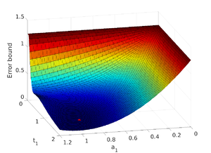
|
| (a) | (b) |
| Figure 15: Error bound for one exponential approximation of the Boussinesq–Basset kernel versus and for both Options A and C. The respective minima are marked with a red dot. | |
Next we study the dependence of the different cost function with respect as and are varied, while and are held fixed to their optimal values. Note from Fig. 16 the convexity of both cost functions with respect to the dependence with respect to the , as compared to . Certainly, to consider only the dependence on makes the optimization problem much more tractable, especially as the dimensionality grows.
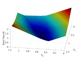
|
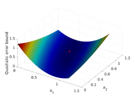
|
| (a) | (b) |
| Figure 16: Error bound for two exponentials as a function of and , with fixed (optimal) and for Options A and C. Options C and D are equivalent in this case. | |
Finally, let us look at the dependence on and alone. Fig. 17 shows a contour plot of the bound in terms of and where, this time, and are being held fixed (at their optimal values). The strong gradients and the nonlinearity of the dependence on the can be clearly appreciated. The cost function is almost flat close to the optimum, but away from it the gradient grows very quickly. This could indicate that the selection of the might not need to be determined with extremely high precision. However, obtaining a fair approximation should be essential. Indeed, we have found in practice this to be the case (see next section).
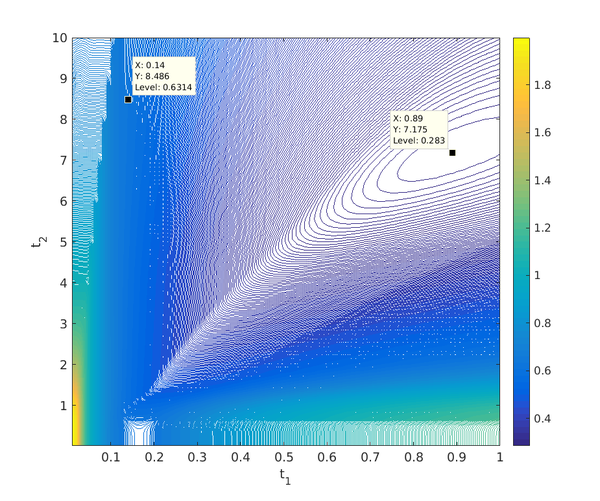
|
| Figure 17: Contour plot of the bound in terms of and . The dependence with respect to the is clearly visible. |
Numerical solution of the optimization problem
In this work we have developed a code in Matlab and solved the problem with a standard PC (3.40GHz processor in a 64-bit architecture). We have nonetheless taken advantage of symbolic coding mode in the Matlab environment to calculate all the derivatives and integrations.
Furthermore, We have also employed the optimization toolbox of Matlab. This tool makes combined use of a variety of methods (Newton-Rapshon, Quasi-Newton and steepest descent, among others) for constraint optimization (box constraints in our case). Continuous optimization algorithms helped to obtain the real (local) minima. Furthermore, their convergence is normally faster than the alternative genetic algorithms. Specifically, we have used the interior point algorithm (primal-dual Newton-Raphson), which considers both the primal and dual variables simultaneously (see, e.g., [261]).
Our numerical experiments show that the problem is full of local minima, thus the strategy of initial point seeding becomes crucial. For each case we must determine and , with . We propose the following heuristic initial point strategy, which has worked well up to , and consists in the following (An upper index is used to refer to the case the parameters correspond to).
- Take randomly generated in .
- For , take as also randomly generated in .
- For , define
(3.48)
This initial strategy is used when solving Options A, B and C. In combination with it, we also employed the Global-search toolbox of Matlab, which is a type of multi-start technique for Global Optimization. This tool granted the possibility of exploring many different initial points and was specifically used with the variables.
Let us make some particularized remarks for the different options:
For Option A the gradient is discontinuous in some regions. So in order to have a robust algorithm, we computed the gradient by perturbations, though at a high computational cost. For Options B and C, the gradient could be computed analytically (symbolically), leading to faster performance. For option D, the gradient is also computed analytically, taking the as specified in Section 3.3.2.
Results
Figure 18, shows the minimized and values of the upper bound for the different options. We have also included the single result reported in [353]. Case C seems to slightly outperform the others, although option A is very close, except perhaps for the last point, where the computational cost was already very high. note that this implies that, at least for the points where , either only local minima were found or convergence had not been achieved when using as the objective function. The complete list of optimized values and corresponding to the and bounds can be found in Appendix F. Let us now make a few comments about these results, looking at each individual option.
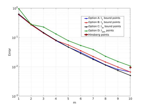
|
| Figure 18: Resulting values of the function for the optimized paramters using each of the different alternatives. The values provided by van Hinsberg et al. for are also shown for comparison. |
For Option A (), for which the gradient is obtained by perturbations, the algorithm suffered significantly for . This was due large number of computations needed to evaluate the gradient, which increases exponentially with when employing perturbations. That is, very sub-optimal solutions were found when the initial values where not set adequately. Precisely this fact justified the convenience of trying large number of initial values and, consequently, the use of Global-search with its associated computational costs. The results come out second-best (after Option C), even though this alternative is the only one that uses the original objective function, .
For Option B and C ( and ), the computational cost per initial point was significantly less, thanks to having an analytical expression for the gradient. Still, finding appropriate initial values remained very demanding. We again observed a strong dependence on initial values and a huge number of local minima significantly hampered the search. Nonetheless, thanks to a reduced cost in computing the gradient, a much larger number of initial points could be employed. As a result, Option C came out slightly on top of Option B and clearly beat Option A and Option D by a considerable margin.
Regarding Option D, number of design variables is halved and, consequently, the number of possible initial values decreases. Though there are local minima, a much smaller number of them were found in this case, which considerably sped up the computations. Nonetheless, the optimized costs were significantly higher that for the other options. Note how, encouragingly, with our proposed strategy 3.3.2 a very similar cost is achieved for compared to that of the parameter set reported in [353].
In general, the bounds monotonically decrease as the number of exponentials increases for all the options, as expected. By looking at particular examples (see Section 3.6), we will see that the actual error also follows the same trend, although not as robustly.
Despite all the technology applied, the problem starts to become unaffordable for for Options A, B and C. The high computational cost is basically caused by the number of required initial guesses, which strongly increases with . This affects all the Options, except Option D, where the problem becomes less severe and the process could actually be carried on further. As we will see, this will not turn out to be necessary in many applications.
3.4 Overall algorithm
We next describe a finite difference discretization of the Maxey–Riley Equation. Our integration scheme of choice is largely borrowed from Daitche [89], who, as we have seen, used the same form of the Boussinesq–Basset force (a Riemann-Liouville half order derivative). A part from the quadrature, it can be classified as a semi-implicit Adams-Bashforth-type method. This type of scheme had earlier been used in [330] where inter-particle collisions were also considered. We have generalized the basic algorithm by adding a quadrature sub-stepping cycle and combining it with Hinsberg's window method (see Section 3.3). Furthermore, our algorithm is written in terms of the absolute velocities (instead of relative velocities), as this is the more convenient form for our DEM-compatible implementation. We focus on the second-order version of the scheme, although we use its first order version for the initial step, as it is commonly done with such multi-step methods.
Let us for convenience rewrite Eq.~2.1 as
|
|
(3.49) |
where stands for the 'non-memory' forces
|
|
(3.50) |
and where now
|
|
(3.51) |
that is, has been split in two: one part has been moved to the LHS of the MRE and the rest has been absorbed, along with , in , which therefore now holds the non-historic contribution from the fluid acceleration. We obtain
|
|
(3.52) |
where
|
|
(3.53) |
The discretization of the integral term in Eq.~3.52 can be done for a variety of finite difference schemes. Here we have chosen the Adams–Bashforth Formulas, as in [89]. On the other hand, the -terms are partitioned according to the MAE, see Eq.~3.16, as
|
|
(3.54) |
and where is calculated with the Daitche method, using the formulas from Section 3.3.1, while is calculated according to Eq.~3.16, Eq.~3.19 and Eq.~3.3. Furthermore, and similarly to what has been done with , the term , which also contains a term proportional to , is split and the latter is sent to the LHS of the equation, leaving the modified term on the RHS. By doing so, the equations become semi-implicit. In the work of [353] it was found that the accuracy and stability of the resulting algorithm improved greatly, avoiding the need for extremely small time-steps. Our preliminary calculations indeed confirmed the same tendency. Denoting the time stepping index as , the resulting first-order scheme (used in the initialization) reads
|
|
(3.55) |
while the second order version is
|
|
(3.56) |
where the subscripts indicate the time-step at which each term must be evaluated and where and extra index ( or ) has been used to indicate which of the formulas, Eq.~3.29 or Eq.~3.30 must be used in each case. The necessity to move to the LHS the part of the discretized added mass force that is proportional to the unknown can be exemplified by the stability analysis of the following simplified equation. Suppose we must discretize
|
|
(3.57) |
where and are negative real values (they resist motion). The naive scheme
|
|
(3.58) |
is unstable for small time steps, as can easily be checked by applying von Neumann's method (see, e.g., [168]). Let us consider a harmonic of the exact solution of the difference scheme Eq.~3.58 at time step to be given by , with the imaginary unit. Replacing each with in the finite difference scheme and dividing through by we obtain the relation
|
|
(3.59) |
which by calling can be expressed as
|
|
(3.60) |
We are interested in the asymptotic behaviour of , so that, unless diverges we can assume and we can write
|
|
(3.61) |
which is asymptotic to
|
|
(3.62) |
as tends to zero. But none of the solutions of the above quadratic equation yield for large enough, and thus we conclude that the amplification factor grows without bound, proving that the naive scheme becomes unstable for small enough time steps.
Going back to the MRE, both expressions Eq.~3.55 and Eq.~3.56 can be more conveniently written as (eliminating the higher order truncation error terms)
|
|
(3.63) |
where takes either the value (first order) or (second order). The flow of instructions that implements the described time integration scheme with the MAE for the approximation of the tail can be expressed as the Algorithms 1 and 2.
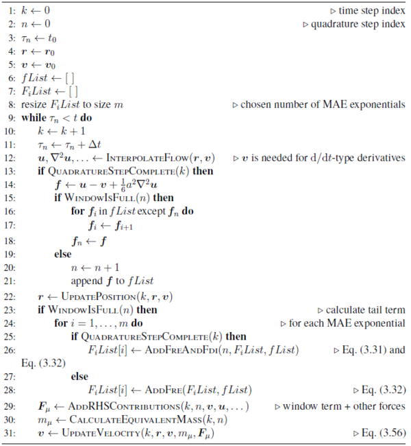
|
|
Algorithm. 1 Time integration algorithm for the MRE: single particle |
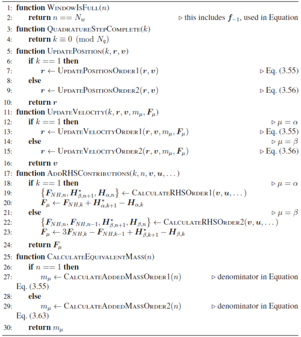
|
|
Algorithm. 2 Implementation of some of the functions in Algorithm1 |
3.5 The fractional calculus perspective
In this section we make a connection between current work on the numerical discretization of the MRE and parallel research in fractional calculus, since we believe it has been missing so far in the literature.
Fractional calculus deals with the generalization of the standard (integer order) differential and integral operators to their analogues of arbitrary, real or complex order [307]. As mentioned in Section 3.2.1, there exist many definitions of such generalized operators [94]. Among those, the most popular are probably the Riemann–Liouville (R–L), Caputo and Grünwald–Letnikov (G–L)-type definitions.
The fractional derivative operators have similar properties to that of their integer-order ones. In particular, the three types mentioned above fulfil: i) linearity, ii) identity of the zeroth-order operator (i.e.its application to a function leaves the function unchanged), iii) backward compatibility (i.e.for integer orders one recovers the standard operators) and iv) index law (i.e.they respect the same composition rules as the standard operators); see [270]. Nevertheless, some important particularities make their treatment more difficult. Among these their nonlocality of the fractional operators stands out.
By writing equations relating various fractional order derivatives, one forms fractional differential equations (FDEs), in an analogy to their integer-order counterparts. Such equations have been used to model several physical processes such as anomalous diffusion [246], viscoelasticity [230], hydrology [36], economics [357] and biological systems [291]; see also the review [339]. In particular, by using Eq.~3.7, the Maxey–Riley equation can be interpreted as a nonlinear system of fractional differential equations, where the only fractional-order term is the history force.
The theoretical study of FDEs has only started relatively recently [201] and its efforts have been focused in generalizing classical results from the theory of differential equations of integer order to the fractional setting. Some significant advances related to the problems of existence of solutions for initial value problems for FDE have been made, see [1,201,102], and, since these works were published, the number of publications in this area has accelerated. It is worth highlighting here the work of Farazmand and Haller [124], who established the existence and uniqueness of weak solutions for the MRE under suitable smoothness conditions; see also [203].
In parallel to the development of the theory, there have been significant advances in the research on numerical methods for the resolution of this type of equations. Most of these consist in adaptations of traditional numerical methods such as finite differences [205], finite elements [319,76], finite volumes [191], spectral methods [130,385], etc. The work [147] summarizes the particular challenges that arise in trying to solve FDEs and some strategies used to overcome them. Again, the nonlocality of the fractional-type operator becomes critical, as it leads to full matrices and full history-dependence, as with the case that concerns us.
New interest in physical models based on FDEs has spurred many developments in recent years [103,69]; see also the broad review by [204]. Specifically, in the field of the numerical resolution of time-fractional differential equations with finite difference methods there have been significant advances, especially geared toward the resolution of multi-dimensional diffusion equations. Many of them focused in obtaining higher-order schemes, since those become more interesting for FDE than they do for standard differential equations, due to their nonlocal nature [69]. The derivative order in most of these works is considered generic, typically in the interval . For example, in [136] (see also [141]) an explicit, second order method is developed based on fractional multi-step methods; first introduced in [226]. Rigorous convergence order and stability analysis are also provided. A different approach based on truncating the infinite series defining the G–L derivative has been chosen by several authors. This method yields first order accuracy in its standard form, but can be enhanced by several procedures. By combining 'shifted' versions of the series, a second order in time and up to third-order accurate in space method was presented in [320]. The method was based on the existence of superconvergent points for the G–L series. A second order in time and up to fourth order accuracy was obtained in [137] with a method based on the same principle. Both methods were applied to diffusion-related problems.
Other authors have focused on making approximations to decrease the huge computational and memory requirements that naturally result for these problems. For instance, in [96,227] the authors make use of the fading history principle or short memory principle (see, e.g., [279]), which states that longer past points have less influence than more recent ones, which allowed them to simply neglect the influence of the former. Note that this is precisely the principle behind window methods. An alternative approach is presented in [209], where the number of time steps in which the solution needs to be stored is distributed unevenly, so that most of the information concentrates closer to the present time. The same work combines this technique Richardson's extrapolation to accelerate convergence. Other methods employ the same concept as window methods by applying different approximations to the convolution kernel for the window region and the tail. For instance, in [207] a method was used that is very similar to the MAE, in that the convolution kernel was in the tail region ('history part' in that work) by a linear combination of exponentials. A different technique is applied in [18], where a multi-pole approximation of the Laplace transform of the kernel is used instead.
However, even today, very few researchers working with the MRE are taking advantage or even mentioning these numerical methods. In fact, the very nature of the history term as a R–L derivative has been ignored for the majority of works on this field. For example, Dorgan and Loth [108] had to rediscover the standard window method, making no mention of the short memory principle nor of fractional calculus altogether. Notably, Bombardelli et al. [40] did make use of the R–L derivative interpretation, presenting their method based on truncating the G–L series (both definitions are equivalent under the studied hypotheses, see [279]). It is nonetheless revealing that these authors do not refer to previous work such as Yuste y Acedo [379], who had used essentially the same method before, although not specifically applying it to the MRE. Similarly, Diethelm et al. [104] (see also [61]) had employed a version of the polynomial/analytic approach later rediscovered by van Hinsberg et al. [353] and Daitche [89] (see also [61]), neither of whom mention these works (or any other works in numerical FDE). In fact, both techniques had been already described in the classic work by Oldham and Spanier [265], where even higher-than-one order G–L series were discussed already. This just goes to show the disconnection that has prevailed between these disciplines.
While the work of Bombardelli et al. was certainly not ignored, it did not seem to have a major impact in the field, due to the modest first-order accuracy that it delivered (although it still improved on previously used methods at the time), as it was soon surpassed by that of [353] and [89]. Nevertheless, we are convinced that the G–L approach can be developed to become more competitive for this problem, since higher-order methods based on this method are becoming increasingly common [320,227]; see also [51], who deals with high-order quadrature formulas. Conversely, we believe that all these works concerned with the numerical treatment of the history force in the MRE can be of value to the discipline of FDE, both in their proposed methodologies and in their role in promoting the visibility of this particular problem. Daitche [89] provided a semi-implicit method with high-order accuracy in time, which can be used to study fractional derivatives of order, not necessarily . Similarly, the MAE might be of use in other areas apart from the MRE (despite it requiring, as it does in its current version, the derivative to be of order ), or at least inspire new methods to approximate the convolution kernel in other contexts.
In summary, the fractional derivative perspective on the analysis of the MRE enriches our understanding of the problem and can inspire future work, although this path has been somewhat neglected in the literature so far. Moreover, we expect the existing approaches to be of value to this broader subject and thus it deserves to be given more visibility. We hope that this section contributes to both goals.
In the next subsection we point to a direction in which the fractional derivative method of Bombardelli et al. could be improved. Admittedly, this section is tentative, but is included to motivate what we interpret to be interesting future lines of work.
3.5.1 Exploring an idea: Richardson's extrapolation
Richardson's extrapolation can be used to transform a sequence of approximants to a new sequence with an accelerated rate of convergence. Suppose that we take a sequence of partitions of the interval given by over which we wish to calculate the quadrature. The partitions are chosen such that each partition contains twice as many subintervals as the preceding one, that is
|
|
(3.64) |
The application of a given quadrature rule over each partition generates a corresponding sequence of approximants
|
|
(3.65) |
where the notation replaces and the zero superscripts indicate the sequence is the zeroth element of a sequence (of sequences), i.e.the zeroth order Richardson sequence.
Now, let us assume the leading term of the error made by a generic can be expressed as
|
|
(3.66) |
so that the error scales with order . Then the first-order Richardson sequence can be obtained by the following rule
|
|
(3.67) |
for , since . Note that the last element of the new sequence formed following this rule is at least one order more accurate than the most accurate approximant in . Note also that the new sequence has one less element and therefore the process can be iterated a maximum of times to obtain ever higher-order approximations.
Richardson's extrapolation does not always work. A review of possible difficulties associated with its use can be found in [52]. The issue of numerical stability and convergence are treated in detail in [315]. We are going to proceed empirically, showing how well it performs for the main quadrature methods seen so far. In general, a very important restriction is given by the fact that obtaining a sequence of partitions such as the one described above, formed by successive powers of two, cannot be achieved in practice in a dynamically changing history of a real simulation. Nonetheless, it is possible to do such a thing with the window method, as the window length can be forced to have the desired number of points. We next show that Bombardelli's method is the best suited for the application of Richardson's technique, turning it into a much more competitive alternative.
Let us, first of all, look at the performance of polynomial interpolation/analytic methods with Richardson's extrapolation for comparison. Since the theoretical order of the error was derived in [89], the corresponding exponents are known and the method can be directly applied. Fig. 19 shows the results for a total duration . The method seems to work best for the first order polynomial case (second order accurate). Its performance becomes comparable to that of order two, but not better. The performance with the other methods is even poorer. The same tendency has been observed for different durations. We suspect this may be due to the piecewise definition of the quadrature formulas, which does not lead to very well-behaved asymptotic error expressions, with perfectly stable coefficients, but more work is needed to establish this point with confidence.
It is remarkable that, in any case, the gains only start to be noticeable after the mesh has become already quite fine. This factor goes against our goal of keeping the set of historic points to a minimum, which requires a very good approximation for the coarsest discretizations.
On the other hand, notice the strong and consistent gains that are achieved by applying the same technique to the fractional derivative approach in Figs. 20-23. Note furthermore how the comparison is more and more favourable to this technique as the total time duration increases.
While we will not pursue this line of research further in this work, we recognize such phenomenon to be an opportunity for boosting the performance of the method. Such a method would be a kind of window method that would consider a number of points in the window region equal to some power of 2. The window contribution would be calculated using Richardson's extrapolation on the Grünwald–Letnikov fractional derivative formula.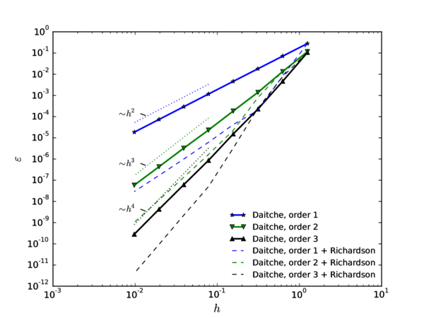
|
| Figure 19: Scaling of the global error of the Daitche method with Richardson extrapolation for |
Let us now analyse the performance of Bombardelli's method with Richardson's extrapolation.
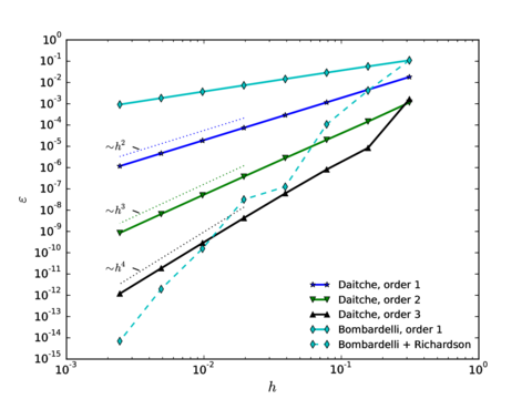
|
| Figure 20: Scaling of global error, |
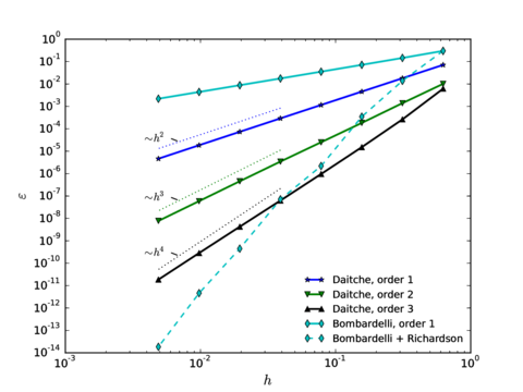
|
| Figure 21: Scaling of global error, |
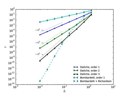
|
| Figure 22: Scaling of global error, |
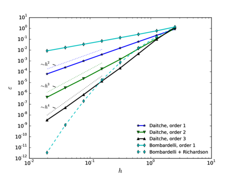
|
| Figure 23: Scaling of global error, |
3.6 Performance of the methodology
In this section we test the performance of the MAE using the optimized and values from Section 3.3.2. We start a with very elementary example, aimed only at measuring the quadrature error. Next, we consider a single-particle example with analytical solution to benchmark the accuracy of the full scheme. The last example features a long-term, 1x10⁴ particle simulation with which we show the remarkable efficiency of the method.
3.6.1 First benchmark: an integral with analytical solution
The error bound Eq.~3.23 can indeed be used for conservative predictions about the expected error when using the MAE. Nonetheless, we wish investigate how this bound in fact relates to the actual error, but of course this can only be done for particular cases. We revisit the same example that we considered in Section 3.2.3. Note that it corresponds to the convolution of the sine function with the Boussinesq–Basset kernel, which may be denoted . This is a very convenient and commonly chosen example, see [40,353,89] 1. Its physical significance is that of a sphere being forced to oscillate in an otherwise quiescent fluid. The error can be expressed, see Eq.~3.23, as
|
|
(3.68) |
since . We have computed the bound numerically, by partitioning the integral in Eq.~3.68 in two parts: an integral over the region where the argument of the absolute value may change and an integral over the rest, where the sign is given by that of (which has a slower asymptotic decay than as ). The first part can be calculated (to very high accuracy) using a standard quadrature method, while the second one has an analytical formula. In order to obtain a representative measure of the error, we evaluate the integral over , with sampled at 40, evenly distributed, points in and we take the mean absolute error within the sample 2. We denote this error as , making explicit its dependence on both and . The results are shown in Fig. 24, where three different sets of parameters are considered: the single list given in [353] (), resulting from the optimization of ; the set obtained from the optimization of , for ; and the set obtained from the optimization of , again for (see Section 3.3.2). For the sake of clarity, we include a single set of results in Fig. 24a where we have picked . Fig. 24b shows the analogous results for a range of window times, including the single curve from Fig. 24a.
Figure 24 shows how indeed the errors fall significantly below their optimized upper bounds, up to more than an order of magnitude so. Overall, it seems that both the and the methods achieve comparable results, while the parameters by van Hinsberg et al. come out as a bit less accurate. Nonetheless, this difference turns out not to be consistently significant, despite our inclusion of the parameters as variables in the optimization problem. This indicates that the trial-and-error strategy used by these authors yielded a close-to-optimal result.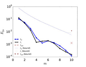
|
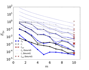
|
| (a) | (b) |
| Figure 24: Error produced by the approximation in calculating for three different sets of values and , corresponding to different cost functions: Option A, Option C and the point given by van Hinsberg et al. The resulting errors are accompanied by their predicted upper bounds. A window time of has been considered in Fig. 24a. Fig. 24b shows the analogous results for different values of corresponing to for (with thicker lines corresponding to larger values of ). | |
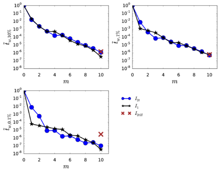
|
| Figure 25: Minimal window time necessary to obtain an error , as a function of the number of exponentials. The time is normalized by the minimal time window required when . |
In theory, the greater the window, the smaller the error should be, because the approximation of the kernel is done over a smaller portion of the total domain. This tendency is expected to be especially pronounced for small values of , close to the singularity of at . There, the well-behaved exponentials have difficulty keeping close to the curve for as it diverges. This is indeed what can be seen in Fig. 24b. The time window ranges 1x10⁻⁵ to 1 fractions of a period and is represented by using greater thickness on the error curves corresponding to larger windows. The tendency of the curves to go horizontal for increasing signals the breakdown of the kernel approximation for extremely small values of . Note that, for smaller than 1x10⁻³, none of our optimal , sets manage to keep the error under the 1x10⁻² mark.
However, a small requires an even smaller integration time step. So as long as the time step is kept large enough, such small time windows become unnecessary, because the memory cost can be afforded. This is why the most effective solution is to use a high accuracy scheme, such as the second or third Daitche schemes for the integration of the window in the MAE.
A final remark about Fig. 24b: note that although the expected monotonous behaviour of the error with respect to variations in is mostly realized, there can be exceptions: for there is a crossing between adjacent sets of curves. This fact highlights the complexity of the relations that govern the method.
A different way to characterize the accuracy gains obtained by increasing the number of exponentials is represented by Fig. 25. It shows the relation between the number of exponentials, and the minimum window time necessary to attain a desired level of accuracy. On the horizontal axis we represent ; on the vertical axis, the normalized window time . The latter is defined as
|
|
(3.69) |
where
|
|
(3.70) |
and similarly we define and . In other words, Fig. 25 addresses the question if is the minimal time window necessary to have less than error when using the standard window method, then what fraction of is instead required when using the MAE?. The answer will depend on the values of and . Strictly speaking, the existence of a unique solution is not even guaranteed, since that would require the strict monotonicity of the dependence of on , which we have seen to only hold approximately. Nonetheless we have applied the bisection algorithm to find such solutions, producing Fig. 25. Note the immense memory cutoffs that are generated by the MAE. For instance, suppose the accuracy goal set to one percent. Then just by including a single exponential approximant, the interval of the particles history that must be tracked is reduced by a factor , by just using the -optimized and . Or else by more than if ten exponentials are considered.
Let us now consider the joint effect of the quadrature algorithm and the kernel approximation, using the same test flow as above. For that, the initial time is taken as , the final time is set to . The time interval is initially partitioned in eighty parts. This amount is successively doubled, defining the range of values of the time step, . For simplicity, the error is now measured at single point (); that is . Fig. 26 shows the performance of the algorithm described in Section 3.4 for a fixed and . The method initially follows the third order slope of the second-order accurate Daitche quadrature algorithm. But then, as soon as the time integration error becomes dominated by the error due to the approximation , its accuracy stagnates, rendering further reductions in futile.
(1) Actually, the convolution of the cosine was considered by [40] and by [353].
(2) Note that the convolution of the sine function is periodic, with the same fundamental period as the sine, as it is readily seen with a change of variable.
3.6.2 Second benchmark: Candelier's solution
There are a limited number of known closed-form particular solutions for the Maxey-Riley equation. Some of these can be found in the works cited in [124]. Fortunately, the solution obtained by Candelier et al. [57] includes the effect of the Boussinesq–Basset force, as well as all the other forces, though the Faxén terms do not contribute in this case. The solution corresponds to the trajectory of a particle that sediments under gravity in an infinite container which is rotating as a rigid solid around a fixed axis. The same benchmark was considered in [89] (see the same work for the input parameters). Fig. 27 shows two spiral trajectories resulting from two different versions of the solution by Candelier and co-workers. The inner spiral corresponds to the full solution, including all the terms in the MRE. The outer spiral is obtained by neglecting the Boussinesq–Basset contribution, while retaining the remaining effects. The asymptotic behaviour of the radial coordinate around the rotation axis is in both cases of exponential form, of which the exponent's coefficient is modified by the presence of Boussinesq–Basset force. This asymptotic solution becomes a very good approximation only after a few turnover times [57]. The exponential form suggests that this test is especially demanding, as it should tend to amplify any systematic inaccuracies over time.
For the purpose of measuring the accuracy of the algorithm, let us define the error function as
|
|
(3.71) |
where is the exact radial coordinate and its numerical approximation. We consider as the measure of the error. This measure has a very similar behaviour to the max-norm over all the time steps. This is because the error tends to accumulate in a monotone way, leading to the maximum value occurring at the final point in most cases; see [89]. For instance, the error introduced by neglecting the Boussinesq–Basset force at is .
Figure 28 shows the error for different values of for the MAE as compared to the bare, second order Daitche method. The optimal points were those obtained with the cost function , since this set gave slightly more accurate results for all values of in this example. We observe that, despite a few permutations do occur between curves with successive values, in general terms increasing yields an increase in accuracy which, on average, amounts to about half an order of magnitude each successive increase.
But, how many exponentials should be used?. Based on accuracy, the safest answer should be as many as possible, or at least, as many as necessary. However, taking efficiency into consideration might complicate the matter. Indeed, adding additional exponentials to the kernel has two detrimental effects on efficiency. First of all, it implies a proportional increase in the total number of operations needed to compute the tail contribution. But more importantly, each new exponential requires an extra vector to be kept in memory per particle, i.e.the value of in the previous step, see Eq.~3.19. Of course it is still possible to increase the time window, thus improving the effectiveness of a fixed number of exponentials, as Fig. 24 suggests. But again, this increase also implies a raise in the memory demand. The situation is summarized in Fig. 29, where the error is plotted against the total number of bytes to be kept in memory per particle. The number of bytes is estimated by assuming that 2.4x101 bytes are taken up by each vector, as
|
|
(3.72) |
where the time step is kept constant at 2.5x10⁻³, close to the saturation time step (below which no further gains are obtained, see Fig. 28). This corresponds to an error of around 1x10⁻³ for 8, 9 or 1x101 exponentials, according to the same figure. The window time is successively doubled, starting at . Again, Fig. 28 shows that only initial increases in the memory demand (via increase in the number of exponentials or the value of ) yield significant gains in accuracy. Furthermore, the gains in accuracy per byte are greater when investing them into more exponentials rather than into additional (except perhaps for the very smallest values of ). In other words, within the analysed ranges, it pays off to take as small as possible, while using as many exponentials as necessary.
Some remarks concerning the choice of tw
It is not quite clear how small is 'as small as possible'. The smallest value considered in Fig. 29 is , or periods. This corresponds to an error of around 1x10⁻³, based on Fig. 26. Making it smaller might very quickly lead to important approximation errors. Furthermore, since the time step is only a fifth of that amount, only five points enter the window region. Any further decrease in would surely damage accuracy, while not significantly reducing the memory requirements, according to Eq.~3.72, with .
Based on this line of reasoning (and our numerical experience), we conclude that ten points are a reasonable option, which we have adopted by default in conjunction to . This translates into 2.1x101 vectors to be stored per particle. Indeed, for a fixed integration time step (which is typically determined by other factors, such as the overall time scheme or the fluid time resolution) the accuracy gain is quite substantial compared to, say, only five points, while still avoiding important memory sanctions. We do recommend this combination as a starting point in other simulations, as long as the frequency of the relative motion is low enough. That is, making sure that at least a few time steps fall within the period corresponding to the highest frequency modes in the motion. For instance, in a turbulent flow, this frequency is that of the Kolmogorov microscales, unless some external, high frequency force is acting on the particle. We test this 10-point, combination in the following benchmark.
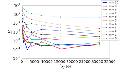
|
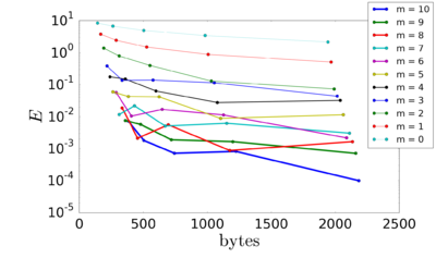
|
| (a) | (b) |
| Figure 29: Relative error of the particle position at the final time () for different memory loads per particle. Fig. 29b is a zoomed-in version of Fig. 29a, showing the intial part with the lesser amount of bytes. | |
Effect of Substepping
Let us test the performance of the algorithm with sub-stepping. Fig. 30 shows the error evolution for different cases in which either the overall time step is modified, or else only the quadrature time step is. Note that the memory requirements per particle associated with the storage of historical values are inversely proportional to the quadrature time step or, equivalently, to . Therefore, scaling either the time step or just the quadrature time step (i.e.) by the same amount imply equal reductions in the memory requirements. However, the accuracy losses are very different. Note that the loss in accuracy for increasing is first only concentrated in the initial stages of the motion, where the whole history is very recent. There the kernel is very large for all the integrated values, amplifying the error. Note that this situation only takes place at the start of the simulation, where the initial conditions of the motion are very uncertain anyway 1.
Note the appearance of oscillations at the start of the simulation. These seem to correspond to amplifications of the error that are introduced when a new historical value is added to the list, as consistently indicates their constant period. Note that these perturbations take place along the whole trajectory, although they become strongly damped after the initial phase (they are still visible for the larger values of ). In any case, the error is always bounded by the error introduced by making the overall time step greater. Note furthermore that the error becomes almost horizontal after the initial phase (joining the reference curve after sufficient time). This indicates that the trajectory of the particle keeps very close to the reference solution (), and that the error is mainly accumulated at the start. indeed, any difference in the estimation of the history force would lead to a different rate in the (approximately exponential) outward motion of the spiral, which would in turn lead to upward sloping errors.
It is not as clear how these gains apply when a window method is used. Indeed, let us assume we wish to keep the number of past contributions, , bounded to ten. To achieve this, we have two parameters to play with: the size of the time window, , and . Making smaller will allow taking smaller quadrature steps, while making bigger will permit increasing and still keep, in both cases, . The increase in brings about a loss in accuracy associated with the quadrature scheme, while a decrease in will require more from the exponential approximation of the kernel which, as we have seen, are a worse approximation nearer the most recent time; thus, some loss of accuracy is expected here too.
The situation suggests the existence of an optimum combination of and , for every given combination of and . We explore this possibility in Fig. 31, which shows the variation of the relative error at as a function of for different numbers of exponentials in the kernel approximation. In each case, the total number of historical data is kept constant at . Note how, as becomes higher, the optimum slightly tends to move left for most of the curves, which corresponds to smaller sizes (smaller ). This is expected, since the greater richness of the exponential kernel makes it better able to approximate the Boussinesq–Basset kernel close to the current time. While all the curves are quite irregular, it is clear that using no sub-stepping at all is the worst option for all but the highest values of and the largest time steps. Overall it seems much safer to take instead of no substepping at all, especially for the lower values.
Clearly, the whole matter of quadrature substepping requires further study, although we have shown the potential of this technique here, especially without the use of a window method. Note that the window method of van Hinsberg et has only been developed for the Basset kernel and is not a matter of a simple generalization to extend it to other kernels. This is not a limitation for the Daitche method, which can be adapted to other kernels [89], like the ones proposed by Mei and Adrian [243] and Lovalenti and Brady [223], which become more accurate for larger values of (see Section 2.2.1). Quadrature substepping could certainly be extended to those situations, where its utility would become much more obvious, given the unavailability of the MAE.
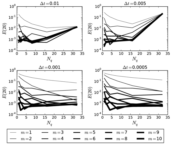
|
| Figure 31: Relative error in the radial coordinate at for a fixed number of historic points () and different number of exponential kernel approximants (). The time step is taken as . |
Comments about the performance of the coefficients by van Hinsberg et al.
The consideration of a generalized optimization problem, in which the coefficients are considered free to vary, does indeed provide more accurate coefficients. The gains in accuracy are in the order of half an order of magnitude (for the bounds) as compared to the simplified problem, in which the coefficients are set according to the simple rule from Eq.~3.48. We ignore the number of iterations considered or what was the heuristic method employed in [353] to fix the before proceeding with the optimization. But the fact our proposed heuristic yields a very similar error (at least for ), as mentioned in Section 3.3.2, is revealing. It seems that while applying the generalized optimization process improves accuracy, it does so only moderately. We have taken the process up to , and so we cannot be sure this trend still holds beyond that point. However, the distance in accuracy between the two approaches does seem to be quite stable, judging from Fig. 18.
The good accuracy of the coefficients by van Hinsberg et al. has been confirmed in the examples considered in Section 3.6.1 and we do not expect this trend to change significantly in other applications. In any case, it is preferable to use the optimal coefficients provided in Appendix F. If the number of exponentials needed was more than ten, using the simplified optimization process (Option C) would be a cost-effective option, perhaps together with the heuristic presented in Eq.~3.48. Due to the accuracy of the MAE, however, in many applications this will not be needed. This is the case of our third benchmark, which we discuss in the following section.
(1) For instance, if the initial conditions are given by the injection of a particle through some mechanical device into the flow, most likely, the presence of such device invalidates the MRE. If, instead, the particle is assumed to have been in the flow before the start of the simulation, then its history is simply unknown and the error will mostly come from this uncertainty in this case.
3.6.3 Third benchmark: Sedimentation through synthetic vortices
We now wish to test the efficiency of the full algorithm. For that, we will consider the benchmark test that was considered in Guseva et al. [155] in their work about the influence of the history force on the dynamical properties of a system of sedimenting particles. These authors studied a synthetic bidimensional flow that is a transient variant of the classic cellular flow field previously studied in, e.g., [239]. The flow field is given by 1
|
|
(3.73) |
where are Cartesian coordinates and and are the characteristic velocity and length-scales of the flow; controls the frequency of the temporal evolution of the flow and k its amplitude. Such flow covers the Cartesian plane with -diameter vortices, each one flowing in the opposite sense than the ones directly next to it.
Guseva and co-workers were interested in studying the long-term evolution of a number of particles subject to the above flow in a double-periodic domain containing four vortices. They monitored 1x10⁴ particles for up to 1.2x10² periods employing the first-order accurate version of the Daitche algorithm. They did not extend the simulation duration any longer, since, as they put it: 'A longer interval is not possible to choose due to the numerical cost of recording the history force with small time step for this number of particles'.
We study one of their examples with the MAE and our optimal points and use it as a test for efficiency. The values chosen for the input physical and numerical parameters are summarized in Table 6 and are roughly consistent with the nondimenional parameters considered in [155], which correspond to the typical conditions in the phenomenon known as marine rain. This term refers to the sedimentation of small agglomerates of mainly organic matter from the surface to the deep ocean, subject to the turbulence found in the upper layers due to the action of wind; see [155] and the references therein. As was done in [155], the effect of Faxén terms will be neglected. Note however that, for the small sized particles considered, such effects are expected to be very small, since
|
|
(3.74) |
And so the effects of the curvature of the flow field around the particle are expected to be very small, since they are expected to scale as the square of this quotient [238].
Figure 32 shows the position of ten thousand particles suspended in the cellular flow at three different time instants. The particles where initially placed in a uniform lattice covering the whole domain, as was done in [155]. The effect of the history force is apparent: With the particles become confined to a set of four curves. In contrast, when including all forces, full bands with particles are still visible at the latest stage, although the bands' edges do become more sharply marked. These qualitative trends are consistent with [155].
Let us now turn to the comparison between the second and third rows in Fig. 32, which correspond to the Daitche method and the MAE, with the optimum points obtained from the cost function . No visible effects arise due to the use of the window method at any of the recorded times, taking . Thus, for this example it is enough to keep around thirty integration points in memory per particle (with a time window of 1x10⁻¹ s ) to capture the qualitative behaviour of the system. In fact, Fig. 35 shows that even less memory would have been required for this example. Notice how for , the solution is virtually indistinguishable from the reference, with .
As a consequence, the total computational time is greatly decreased, as is made apparent by Fig. 36 (compare the full, black curve to the green curve), where the elapsed time per unit simulated time is represented. The steady increase in memory resources and the number of computations per time step translates into ever higher costs for the Daitche method. The MAE, instead, stabilizes after a few time steps, once the window region is completely filled. Note that in our implementation the cost is of the same order as for the case of neglecting the history force altogether.
Admittedly, our implementation is mounted on top of a 3D discrete element code, where neighbour search has been switched off. The flexibility of the application sacrifices some efficiency and thus one cannot conclude the latter statement to be the case in more optimized implementations. Indeed, more detailed analyses with the help of profilers show that a vast majority of the time spent in computing the hydrodynamic forces is still being spent with the history force. Further analysis and reductions of the history force cost are thus in order. However we have demonstrated that the MAE, as described, already critically improves the situation. The perspective of routinely including the Boussinesq–Basset force in the numerical implementation of the Maxey–Riley seems now much closer.
Similarly, Fig. 34 shows the effect of using quadrature substepping on the evolution of the same cloud of suspended particles. To simplify the matter, we do not use the window method here. The snapshots correspond to , where the changes become most evident. Furthermore, only the top right cell is shown, taking advantage of symmetry, which was preserved in all the studied cases. Note that the overall shape of the different ensembles remain remarkably stable up to . At the deterioration of the approximation becomes clearly visible. At the topology of the attractors seems to change and a doubling of the limit lines arises. This corresponds to a quadrature step of 7.2x10⁻¹ periods of the cyclic motion.
The effect of quadrature substepping on efficiency is clear: each time the quadrature time step is doubled, the cost of each time step decreases (see Fig. 36). Furthermore, the effect is most effective after the first increases, as the memory requirements are reduced enough to relieve the memory bottleneck. A small amount of quadrature substepping can therefore provide a great deal of numerical benefits, while introducing only minimal inaccuracies if it is kept moderate enough. We conjecture that the maximum allowable amount of substepping can related to the smallest scales in the flow, at least in an order-of-magnitude sense. That is, the smallest time scales must be resolved with a sufficient number of quadrature points to have an accurate method. More work will however be needed to produce concrete rules, applicable to a wide range of applications.
| Parameter | Value | Description |
| 9.81 m s-1 ^2 | gravity acceleration | |
| Flow parameters | ||
| 3x10⁻¹ m s-1 | characteristic velocity | |
| 1x10⁻¹ m | characteristic length | |
| 2.72 | trans. amplitude parameter | |
| trans. frequency parameter | ||
| 1x10³ m-1 ^3 | fluid density | |
| 1x10⁻⁶ m ^2s-1 | fluid kinematic viscosity | |
| Particles parameters | ||
| 3.9685x10⁻⁴ m | particle radius | |
| 1.5x10³ m-1 ^3 | particle density | |
| 1.72x10⁻¹ m s-1 | terminal settling velocity | |
| Numerical parameters | ||
| 3x10⁻³ s | time step | |
| 1x10⁻¹ s | time window (for MAE only) | |
| 1x101 | number of exponentials (for MAE only) | |
|
|

|

|
| (a) m=0 | (b) m=3 | (c) m=6 | (d) m=10 |
| Figure 35: Detail of a quarter of the domain shown in 32 at for different number of exponentials used to approximate the tail with . | |||
(1) The flow described in [155] differs from the one described here in that, in it, the arguments of the sine and cosine functions are pre-multiplied by . We however only managed to obtain similar results to the ones reported in their work upon removing this factor. We suspected that the difference was simply due to a misprint. In contacting the authors, this possibility was given credibility and thus we have assumed this to be the case. Note that, in particular, this modification changes the meaning of , which is no longer equal to the diameter of a vortex, but rather times smaller.
3.7 Summary
In this chapter we discuss the numerical solution of the Maxey–Riley equation, of which we assume the fluid field variables to be available at the particles' locations. Our main interest is the simulation of the large ensembles of suspended particles that commonly arise in the study of particle-laden flows, for which efficiency is paramount. Thus, having identified the Basset–Boussinesq history force as responsible for most of the overall computational cost, we have concentrated on its treatment.
We have presented an algorithm that combines the higher order quadrature scheme presented in [89] (Daitche method) with the window method presented in [353] (MAE). This algorithm is designed to minimize the huge memory resources needed to include the history force. This is a common problem encountered in the field of numerical methods for fractional differential equations, due to the intrinsic nonlocality of fractional-order integro-differential operators. This observation motivated the inclusion of the review in Section 3.5, where we establish a connection with parallel research in that field. This had notoriously been missing in the literature dealing with the numerical simulation of the MRE, despite the existing wealth of promising resources in this area.
In order to exemplify the potential of the fractional calculus perspective, we tentatively explore the possibility of introducing Richardson extrapolation to boost its order of approximation in Section 3.5.1. For a fixed final time, this technique works remarkably well with the Grünwald–Letnikov (first-order-accurate) method of Bombardelli et al. [40], yielding slopes in excess of four in the semi-logarithmic error plots. However, in a realistic setting the final time would be constantly being updated and thus the number of history points would change, precluding a literal implementation of the method. Nevertheless, there exists the possibility of using a window method to precisely control the number of points in the window region, although have not pursued this line of research, leaving it for future work.
In Section 3.3 we present several enhancements to the MAE. First, the concept of quadrature substepping is introduced to substantially reduce the number of historical data that must be stored by using different time steps for the quadrature and for the time integration schemes. We generalized the Daitche method to allow for this, of which the corresponding formulas are given in Section 3.3.1. It is shown that a small amount of substepping induces small increases in the numerical error, much less than an equivalent increment of the overall time step. Such strategy might come in very handy when the MAE is not available or lacks accuracy, such as when the history kernel is not of the Boussinesq–Basset form.
Second, we have generalized the original formulation of the MAE by including all the free parameters in the optimization, In the original formulation, half of the parameters (the ) where determined by solving an optimization problem, while the other half (the ) had to be fixed based on heuristic arguments. In our approach both sets of parameters are treated as unknowns, widening the space of possible solutions. Furthermore, we have considered a range of cost functions, including the norm of the error () which was replaced by van Hinsberg et al. by a differentiable function ().
It turns out that the resulting problem is significantly more challenging. To address it, We have combined advanced optimization techniques with relatively large computational resources, producing the list of parameters summarized in Appendix F and ready for implementation in particle-laden flow simulations (see Appendix F). By extending the problem, we have introduced a strategy that could inspire future research to continue refining and/or extending our list.
The results show that there is not much to be gained in using the error norm since it produces results of similar accuracy to that of , a more tractable function. The inclusion of the coefficients in the analysis does improve the accuracy in up to half an order of magnitude (in the optimal error bounds), which is a modest gain that we have shown to depend weakly on the number of exponentials, .
In any case, using our list of parameters the overall algorithm already delivers a very high performance. We have shown this in several tests, where the method displayed remarkable accuracy. We have demonstrated that the reductions in the memory requirements can consistently be expected to exceed three orders of magnitude, even when the accuracy requirements are strict. As a consequence, the computational cost of including the history force has not changed the order of magnitude of the overall performance of the code in a long simulation with 1x10⁴ particles. We find this result remarkable, since it is an extended view that the inclusion of this force dramatically hinders performance. Furthermore, we have seen that with a very small number of exponentials we may already achieve the necessary accuracy. For example, in the marine rain example, taking was sufficient to correctly predict the form of the attractors. This fact may become crucial for the viability of many memory-thirsty applications, such as in long-term, large-scale particle-laden flows simulations.
From our work in this chapter we conclude that thanks to the methods we have tested and improved, the possibility of including the history force in practical particle-laden flows is probably close to becoming realistic. The practical implications of this will be particularly relevant to the simulation of liquid-solid flows, were the importance of this force has been proven in a number of studies.
4 Forward and backward-coupled particulate flows
4.1 Introduction
The work presented in this chapter has been developed as part of the activities most closely associated to the company's side of the Doctorat Industrial. The work has been driven by mixed forces. On the one hand, the pursue of the scientific goal of exploring the possibilities of an FEM-DEM framework, which had been left virtually unexplored in the literature. Indeed, the practical totality of reported simulations of particle-laden flows using the Euler–Lagrange approach model the fluid using one of following techniques: finite volumes[371,387], lattice-Boltzmann [333] or pseudo-spectral [331] methods.
On the other hand, the need to deal with the constraints of industrial demands strongly shaped the evolution of our application SwimmingDEMApplication and the type of problems presented here. As a result, this chapter is mainly application-oriented, with the occasional presentation of related research that has been undertaken to meet the needs arisen during the development of our numerical tool.
The referred applications are thus not always smoothly linked to the theory presented in Chapters 2 and 3. Certainly, we do apply the algorithms developed in Chapter 3 and also draw knowledge from Chapter 2. But industrial demand is rarely fully aligned with one's previous research. As a consequence, for instance, none of the presented applications fall within the range of applicability of the MRE. We do however apply an extended version of the equation, see Section 4.2.
Up to this point, it has always been assumed that the background fluid flow field was known at the particles' positions. In this chapter we will be concerned with how to obtain the required flow information from the solution of a finite element computation. The field in the MRE will therefore be considered an unknown from now on.
Our numerical method is based on the point-particle approach (see e.g. [85]), where the flow disturbance caused by the particles is considered a fine detail and is not resolved by the computational mesh, but at most averaged and spread over the mesh nodes based on a filtering technique (see Section 4.8). The particles are treated as Lagrangian points and their motion is integrated based on some variant of Eq.~4.1 (the MRE). This requires knowledge about the background fluid field (the velocity and perhaps its derivatives) at the location of the particles. Since the fluid is not resolved around the point-particles, the computational mesh needs not be any finer than several times the particles radius, as long as the macroscopic behaviour of the fluid is well-captured (see Fig. 37).
Since we use finite elements, the flow velocity field is defined everywhere in the domain and it can be easily calculated as a linear combination of the shape functions. By using a search algorithm very similar to the one employed for the neighbour search [216], every particle is assigned a fluid element, so that only the non-vanishing shape functions need be taken into account in calculating the velocity. The details are presented in Section 4.5. The calculation of the fluid derivatives involves the application of recovery techniques described in Section 4.4.
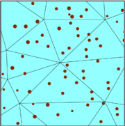
|
| Figure 37: Point-particle approach illustrated. The radius of the particles is only relevant to their contact, not to the fluid interaction, for which only their center point is of relevance. |
There are several levels at which the interactions between the different phases or, more generally, components [109], could be considered theoretically. Fig. 38 shows a conceptual diagram of these interactions. With full line arrows we show the interactions typically considered in the one-way coupled strategy. Those include the forward coupling of the particles to the fluid, whereby the particles are moved according the calculated fluid velocities but the fluid is insensitive to the particles. Optionally, a one-way coupled simulation may also take into account the contacts of the particles with the solid boundaries. These boundaries often coincide with the Dirichlet boundaries for the fluid problem; i.e.forward fluid-structure interaction (FSI). We also mark the inter-particle contact interactions with full lines, since it is our default setting, although this can be treated separately and is sometimes referred to as four-way coupling [84]. The one way coupled strategy is adopted in the first part of this chapter.
In the second part of the chapter we are concerned with two-way coupled flows, where the movement of the particles affects the fluid phase in two ways. First, the relative motion of the particles with respect to the fluid generates a force that is applied back to the fluid, using a filtering technique. Second, the mass conservation equation is altered to account for the volume occupied by each phase. Both these interactions are indicated with dotted lines in Fig. 38.
We have ignored other possible interactions in this work. First, we do not consider the effect of the fluid on the structures (backward FSI) or the self-contacts between structural parts. Second, we have neglected the hydrodynamic interactions that result from the interactions between the sub-scale fluid perturbations and the particle. This type of actions has been termed three-way interaction [84]. It requires the introduction of special methods that take into account the relative position of particles, such as the simple superposition method (see [363] and references therein) and its more sophisticated variants [15,292] or the expensive (though very accurate) Stokesian dynamics [43,316], all of which are based on the low particle Reynolds number assumption and most on the Stokes flow assumption. Other, empirical techniques have been proposed to capture a rough estimate of the hydrodynamic interactions, including the case of higher particle Reynolds numbers. Most of these techniques are based on the idea of modifying the drag coefficient using the local average of the particles' volume fraction [31,378].
Note that it is not clear whether the latter method should be classified as three or two-way coupling, as it involves a calculation of a fluid-average quantity (the volume fraction) that is then projected onto the particles. So, ultimately, it is the fluid field that is being modified if one counts the solid fraction as a variable of the generalized fluid phase. Moreover, this type of modification has the same resolution as the fluid, while the individual particle perturbations remain below this scale. In this sense, it could be seen as two-way coupling. Note that we have already come across this conceptual overlap of the one and three-way coupling interactions in Section 2.2.4. In any case, we do use this technique in our last application example, Section 4.9.4.2 Beyond the MRE
As hinted in the introduction, it is possible to modify the MRE to extend its range of applicability beyond that analysed in Chapter 2. For instance, the first-order inertial effects, discussed in Section 2.2.1 may be incorporated, leading to more complicated expressions for the different forces that still fall back to the ones in the MRE in the very low limit. We mentioned the work of Lovalenti and Brady [223], where such task is undertaken. In [224] the task is generalized to arbitrary time-dependent motions of a sphere in uniform flow, giving the exact formula for the hydrodynamic force to order .
Such analytic models become increasingly complex very quickly and yield increasingly costly and complicated expressions. Furthermore, their generality is often not sufficient and so their practical application is relegated to very specific (though in many cases very relevant) examples. More importantly: their range of application is usually small, as nonlinear effects start to become more and more dominant. For instance, the expressions provided in [224] are only valid for . It is for these reasons that we have left their discussion out of the scope of this work. The problem is that there are still many applications were the particle Reynolds numbers (and other nondimensional numbers as well) exceeds the limits studied in Section 2.2 or any of the analytical formulas available.
An alternative to these analytical formulations is provided by empirical models. The usual form of these models is analogous to that of the MRE (or its analytical extensions), such that for each term in the latter, there is a modified analogue in the former. The most common way to apply such a modification is to premultiply the original term by a scalar function that is a function of the relevant nondimensional numbers that fall outside the referred range of applicability. The constant parameters are fixed by running experiments that also serve to determine the range of applicability of these expressions. Note that these empirical models are a new theory and have to be held as such. That is, they do not logically follow from more fundamental theories (such as the Navier–Stokes equations) just as the MRE equation does. This means that, in particular, it should be checked that
- Each term in the resulting equation has been validated in its own range of applicability
- The particular additive decomposition of forces is correct (are the chosen terms mutually compatible?)
- The uncertainty related to the possible unsteadyness of the flow is compatible with the required accuracy
The first item above is the most obvious: now each force is a model in itself and it should be a validated one. With respect to item 2, note that the additive combination of the different forces stems from the mathematical analysis of the problem in the case of the MRE, while here it becomes an assumption. Finally, Item 3 refers to the fact that the chaotic motion of the fluid that arises at higher Reynolds numbers 1 implies that the deterministic models for the different hydrodynamic forces can only be interpreted as ensemble averages, which means that some dispersion is inherently linked to them and this should taken into account.
These are not the only issues related to the use of these models. For instance the presence of ambient turbulence [33] and the proximity of neighbouring particles are examples of effects that can play an important role but that are difficult to characterize reliably. The second of this areas has probably received the most attention and is currently very active area of research, with a large number of new models being continually proposed [31,378,99,317]; see [393,208] for models proposed to take into account the effect of anisotropy in the distribution of neighbours.
We next summarize the form of the expressions of the most relevant extensions for practical purposes (certainly for the present work). We follow closely the most comprehensive exposition that has been given on the subject to date, put forward in a series of reviews by Eric Loth and co-workers [217,218,222]. These authors considered the following form of the equation of motion for a small but finite sized particle, ignoring all body forces but the weight, by the an equation of the form
|
|
(4.1) |
where is the mass of the particle, where is the sum of the contact forces due to current particles or solid walls that overlap with the target sphere; and where denotes the hydrodynamic force (discussed below) and the buoyancy force, given by
|
|
(4.2) |
where is the mass of a volume of fluid displaced by the particle and where the hydrodynamic force is given by the following combination [222]:
|
|
(4.3) |
Furthermore, in some situations it is important to include the rotational degrees of freedom. The angular equation of motion reads
|
|
(4.4) |
where is the moment of inertia of the particle (a scalar for a sphere, otherwise the whole inertia tensor should be used), where is the sum of the moments due to the contact forces (sometimes also moments) between overlapping particles and particles and solid surfaces. The hydrodynamic moment is discussed below.
Note that Eqs.~4.1 and 4.4 neglect hydrodynamic interactions between neighbouring particles, the aforementioned three-way coupling. For possible extensions to include these effects see [15,292]. The different forces and torques above are next detailed.
(1) Indeed, above the wake behind a sphere immersed in uniform flow becomes unsteady, as tested through physical and numerical experiments, see [187,74] (note that the Reynolds number is based on the diameter in these works) .
4.2.1 Unperturbed fluid and added mass forces
The validity of the MRE requires that the particle Reynolds number is smaller than one, as we have seen in Chapter 2. At the opposite extreme, in the inviscid limit, valid for vanishing viscosity, the equation of Auton et al. [14] applies, which is in the form Eq.~4.1 (ignoring the contact terms). In this case the hydrodynamic force reads
|
|
(4.5) |
where the forces with the same subindices as in Eq.~2.1 denote forces with the same physical meaning.
Let us now discuss the particular expressions of each of the first two terms above. First, has exactly the same form in both limits. Its physical meaning is clear: what is the force that the sphere of fluid displaced by the particle would feel if taken as a point-mass? It would correspond to its mass, , multiplied by its acceleration, that is, the material acceleration of the background fluid field, as measured at the center of the sphere. Thus, this force reads
|
|
(4.6) |
where the capitalized derivative operator denotes the material derivative. Loth [219] argues that the fact that the expression of is valid in these two regimes confirms that the expression should be robust generically, and so we will assume so.
Similarly, with respect to the added mass force, the following expression is valid both in the inviscid and the vanishing particle Reynolds number limit
|
|
(4.7) |
Moreover, there is considerable evidence of its accuracy outside the theoretical range of validity [361,194]. We thus assume this form of the added mass force to be valid for the complete range of Reynolds numbers too.
4.2.2 Drag force
The drag force can be defined as the ensemble-averaged force experimented by a particle submerged in a statistically stationary flow in the direction of the relative velocity between the particle and the far-field averaged flow velocity. It can be expressed as
|
|
(4.8) |
where is the cross-sectional area of the particle for a section orthogonal to where the drag coefficient is in general dependent on , the shape of the particle [218], the local solid fraction [31] and the properties of the fluid (see Section 4.7.3). This formulation is trivially a generalization of the Stokes drag, for which .
4.2.3 History force
The history force can be defined as the transient component of the viscous force that is parallel to the drag force [223,222]. This force is associated to the transient development of the flow field in the vicinity of the particle. It depends on the particle's relative velocity history, because of the finite-speed of vorticity to convect from the particle surface and away from it. A generic form of this force, which covers the analytically derived form of in the MRE and also the empirical model of Mei and Adrian [243], of widespread popularity and valid for particle Reynolds numbers up to about 2x10²; is given by
|
|
(4.9) |
where we have used the result proved in Appendix C to take the derivative outside the integral sign. Note that for we recover the MRE expression for the history force (with no Faxén terms).
4.2.4 Lift force
For flows in which the shear dominates the rigid solid motion 1. A generalized formula for the lift force due to shear in the flow is given by [219]
|
|
(4.10) |
Similarly, for spin-induced flow one has
|
|
(4.11) |
where the nondimensional particle angular velocity is defined as
|
|
(4.12) |
The linear addition of the two effects (lift due to shear and lift due to spin) has been seen to be reasonable for value as high as and [219].
(1) Note that, according to Section 2.2.1, there is a distinction, for small values of between vortex-induced lift (due to the flow's solid body rotation) and shear-induced lift. Here we omit this distinction for simplicity given that, in most flows, the shear-induced component is much more important [219]. Furthermore, the distinction disappears at the inviscid limit [13].
4.2.5 Torque
If the particle angular degrees of freedom are to be tracked (to calculate the lift, for example), then the hydrodynamic torque must be accounted for in order to predict the angular velocity. Following [34], the expression of such torque can be approximated by
|
|
(4.13) |
where and are empirical coefficients that tend to one for , recovering the analytical solution of Rubinow and Keller [294], valid in this range. The validity range of this linear addition of effects has been proved to be accurate for when the particle's angular velocity does not differ too much from the equilibrium velocity, i.e. [219].
4.3 The continuous-phase problem
Let us begin by describing the problem corresponding to the continuous phase when considered uncoupled to the disperse phase. For the moment, we restrict our attention to incompressible, Newtonian fluids, such as air or water at low speeds. Their motion is accurately modelled by the Navier–Stokes equations:
|
where is the fluid velocity, is the pressure and is an external body force (for example, gravity). As in the previous chapters, is the fluid density and its viscosity (both of which we assume to be constant). The corresponding initial, Dirichlet and Neumann boundary conditions are given by
|
where must fulfil Eq.~4.14.b, where the domain's boundary is partitioned as , , with the exterior unitary normal vector on ; where is the imposed surface traction and where the Cauchy stress tensor is defined as
|
|
(4.16) |
with and
|
|
(4.17) |
where is the deviator stress tensor.
4.3.1 Variational form of the problem
Let us present the variational (weak) form of Eq.~4.15.a, from which the FEM is derived. In order to do so it is convenient to fix some notation. The space of square integrable real functions in is denoted by and the space of functions whose first derivative is square integrable is denoted by . let be the subspace of functions in vanishing on (the boundary of ). The vector counterparts of these spaces are denoted with bold characters. For example, is the space of vector variables with zero trace at the boundary. In this context, the dimension of the vectors is given by . Furthermore, let be the space of functions in that fulfil the Dirichlet condition Eq.~4.15.b. Finally, we are interested in time varying functions, and so we define, for a generic space , as the space of functions such that, restricted to a fixed time in , are members of and, restricted to a fixed point in , square integrable time functions in . With these notations, the weak version of the problem formed by Eq.~4.14.a and Eq.~4.15.a is to find with and such that
|
|
(4.18) |
for all in , where ; where denotes the inner product in ; and where the integral of the product of the two functions, defined in the spaces where it makes sense (normally is assumed to live in the topological dual of ) .
The basic strategy in the FEM is to replace the relevant (infinite-dimensional) spaces of functions above with finite dimensional counterparts in the variational version of the problem, leading to the algebraic system of equations that must be solved computationally. In this work we wish to use the simplest linear simplex elements, both for the pressure and for the velocity. However, not all element combinations lead to converging numerical methods for mixed problems and, in particular, a necessary condition to achieve it is that the particular combination of finite element spaces fulfil the inf-sup or Ladyzhenskaya-Babusska-Brezzi (LBB) condition. This condition can be stated as
|
|
(4.19) |
where and are the spaces containing the velocity and pressure solutions respectively and is a positive constant. In particular, the equal-order, piecewise linear spaces for the velocity and for the pressure ( element) do not fulfil this condition [119]. However, one can resort to stabilization methods to allow for this by modifying the weak form of the problem. We delay the presentation of the weak version of the equations above from which the finite element systems of equations are derived, which is instead presented in Section 4.8 and is not essentially relevant at this point. We thus jump to the discretization associated with our finite element strategy, since the phase coupling is based on it.
4.3.2 VMS-stabilized finite element formulation
Variational multiscale (VMS) methods [174,77] provide a theoretical framework for the development of stabilized finite element formulations. They are based on the explicit consideration of the decomposition of the continuous solution into a part belonging to the finite element space and its complement in the continuous solution space, or subscale. The general strategy consists in modifying the standard FEM solution by taking into account the effects of the subscales in the solution, in a way that is reminiscent of LES turbulence models, where the unresolved scales provide terms that alter the large-scales flow, even though these scales remain unresolved [82]. In this subsection we introduce the essential ingredients involved in the formulation of a VMS-stabilised FEM method. This formulation is used for the simulation of the one-way coupled fluid simulations, but is also relevant to the development of the two-way coupled equation discussed in Section 4.8, after modification of the appropriate terms.
Finite element essentials
Let us consider a conforming finite element partition of the domain . For each element in the domain we denote its diameter as and we define . With these tools it is possible to construct the finite element spaces in the usual way, as , with , . The finite element solution will be a function . Since we will be using equal-order spaces for the velocity components and for the pressure, the solution can be expressed as (summation is assumed for repeated indices)
|
|
(4.20) |
for and ; where the are the shape functions, is the number of space dimensions ( or ) and is the total number of mesh nodes.
Subscale decomposition for a general convection-diffusion-reaction system
Eq.~4.18 is nonlinear due to the convective term, and it will need to be linearised. Let us thus next consider the already linearised version of the Navier–Stokes system, assuming that the convective velocity is a given . In practice, will be taken as its value from the previous iteration, but leaving the formulation unspecified has the advantage of allowing the consideration of different definitions of this convective term; see [82]. The formulation presented next is not new, but we need to describe it in sufficient detail and in a way that is general enough to include the formulation that is later presented for the two-way coupled flow. We are interested in solving the following problem given by
|
|
(4.21) |
together with the boundary conditions from Eq.~4.15.a, and where
|
|
(4.22) |
where the usual summation convention is implied upon repeated indices.
For the particular case of the (linearised) Navier–Stokes equations, the different vectors and matrices are defined as
|
|
(4.23) |
and the matrices , and are matrices () which, for the case are defined as:
|
|
(4.24) |
|
|
(4.25) |
where, as is conventionally done, we have divided through by the fluid density and redefined the pressure as itself divided by the density. Assuming the fluid density is constant, the variable disappears from the formulation.
The weak form of the problem can in turn be expressed as find such that
|
|
(4.26) |
which is equivalent to
|
|
(4.27) |
Adding all the terms above and taking into account that the Neumann boundary terms must add up to the known traction on the boundary times the test function (since they arise from integrating by parts an expression of the divergence of the stress tensor), we obtain the following expression for the weak form of the problem
|
|
(4.28) |
where
|
|
(4.29) |
and
|
|
(4.30) |
As mentioned above, the direct consideration of equal-order finite element spaces to approximate the spaces of the velocity and the pressure in Eq.~4.27, would result in an unstable method. We must therefore modify the problem somehow and the VMS method provides an effective answer. The method starts by considering a decomposition of the solution space as , where is the FE space and can be any space to complete the FEM space in . We assume that functions in already vanish on the Dirichlet boundary (the finite element approximation is perfect there), so that . is called the space of subgrid scales or subscales. Note that Eq.~4.26 is equivalent to find and such that
|
by applying Stokes' theorem to the elemental volumes, recognizing the continuity of the exact tested functions and neglecting the contribution of the inter-element boundary integrals that appear when applying the theorem to , the equations above can be replaced by
|
|
(4.33) |
and
|
|
(4.34) |
where the formal adjoint of operator , denoted by , can easily be computed by transposing matrices , and and multiplying the odd-order derivative terms by [120].
Now, a key insight is to realize that Eq.~4.34 implies there exists a , where the super-index indicates orthogonal complementarity of the space with respect to the -norm; such that
|
|
(4.35) |
for every elemental volume in the domain; where we have defined . The objective at this point is to provide an approximate solution to Eq.~4.35 in terms of . The resulting expression is then to be introduced in Eq.~4.33 to produce a stabilized method. Different expressions for produce different variants of the VMS, as we show below.
There are several options. One is to provide a finite difference approximation to the dynamic term of the subscales above. The particular time discretizaton is not essential and it certainly does not need to coincide with the overall problem's time discretization, which is discussed below. Here we use a backward Euler strategy, although more general schemes are considered elsewhere [78]. Introducing this time discretization into Eq.~4.35 yields
|
|
(4.36) |
The equation above is then approximately solved by assuming that the operator can be approximated by a linear transformation represented by an invertible matrix within the element . In this case an expression for is given explicitly by
|
|
(4.37) |
The design of the matrix is one of the most relevant distinctive features of different stabilization methods. Here we adopt the model proposed in [78], where it is motivated by Fourier analysis of the subscales. Most importantly, optimal convergence can be proved for the present problem under the usual existence and smoothness assumptions (see [77,78]). The stabilization matrix for the Navier–Stoke problem is given by
|
|
(4.38) |
where
|
|
(4.39) |
where
|
and where the constants and are numerical constants that are often taken to be [82].
Determination of the subscale model
Our approximate equation for the subscale Eq.~4.37 depends on the value of . This function is unknown and its determination depends in the specific decomposition chosen. There are many possibilities, but the specific choice (space of orthogonal subscales) leads, after a number of approximations (see [78]) to and . The latter condition means that . Using Eq.~4.37 this condition implies that
|
|
(4.42) |
or, equivalently,
|
|
(4.43) |
where is the inner product defined by
|
|
(4.44) |
Substituting this expression into Eq.~4.37 we have
|
|
(4.45) |
Which defines the subscale model corresponding to the orthogonal subscales (OSS) method by Codina [78]. By instead taking ; i.e.by neglecting one recovers the algebraic sub-grid scales (ASGS) method [77] . Both method have similar stabilization properties, with the ASGS adding a little more diffusion.
Final stabilized formulations and simplifications
A possible simplification of the above formulation is to approximate , where denotes the projection within the element interiors. This simplification disregards the effect of differences in the element sizes and is thus expected to work better the more homogeneous the finite element mesh is. Taking this assumption leads to the following equations for the OSS case:
- (We will assume that is a finite element function)
- (Since is a finite element function)
- (Since is orthogonal to )
Once the model for the subscales has been established, the stabilized method is obtained directly by substituting the corresponding expression in Eq.~4.31, which, for the OSS method and taking into account the above equations, yields
|
|
(4.46) |
The above equation can equivalently be written as the system
|
|
(4.47) |
where is the -projection onto the finite element space (which coincides with the -projection for uniform meshes). This suggests the possibility of solving the system in an iterative, staggered way, using the values for from the previous nonlinear iteration (see Section 4.3.3). In order to make the formulation clearer let us introduce
|
|
(4.48) |
|
|
(4.49) |
The method above is the dynamic-OSS method. Neglecting (and also neglecting the term dependent on the time step in the definition of ) results in the quasi-static version of the method (Q-OSS). Both methods are viable stabilized numerical methods for the Navier-Stokes equations. However, for very small time steps () it becomes necessary to track the subscales [78]. In practice, it is possible to neglect and still consider the terms dependent on the time step in the definition of . However, this results in an inconsistent method, which must be taken into account.
The final expression of the variational problem, assuming a staggered resolution of Eq.~4.47 reads
|
|
(4.50) |
where the stabilized bilinear form is defined by
|
|
(4.51) |
and where
|
|
(4.52) |
The ASGS method is obtained by taking , which results in the following problem
|
|
(4.53) |
where the stabilized bilinear form is defined by
|
|
(4.54) |
and where
|
|
(4.55) |
4.3.3 The overall algorithm
The spatial discretization of Eq.~4.18 is obtained through the use of linear tetrahedral elements, stabilized with the variational multiscale stabilization technique [174,77], which leads to an optimal, second order mesh-size convergence. The particular variant of the method that we use here corresponds to the stationary subgrid scales (Q-ASGS) formulation, which is described in full detail in [82]. After assembling all the elements contributions and imposing the boundary conditions, it leads to a system of equations of the form
|
|
(4.56) |
where and stand for the nodal unknowns for the velocity ( unknowns) and for the pressure () for the pressure respectively. For the time discretization we us a second-order, Bossak time integration [370], defined as
|
|
(4.57) |
|
|
(4.58) |
where is the time-step index. Combining both equations in Applying this scheme to Eqs.~4.57 and 4.58 one obtains
|
|
(4.59) |
where we choose and 1 and where we have defined the residual . The nonlinearities present in Eq.~4.14.a are linearised using a first-order Taylor expansion. That is, at each nonlinear iteration one solves for the :
|
|
(4.60) |
Then the solution and residual are iteratively updated with Picard's method as
|
|
(4.61) |
where the index represents the nonlinear iteration count and where, in evaluating the derivative of the residual, we use the following approximation
|
|
(4.62) |
where the indices are applied only to matrix , as does not depend on the solution. Note that this approximation assumes that the variation of is moderate compared to that of the solution vector itself, otherwise convergence problems can appear. Consequently, the final system to be solved is
|
|
(4.63) |
(1) This combination of parameters provides good damping properties of the highest frequencies and robust behaviour overall, see [370].
4.4 Derivative recovery
The procedure by which one obtains approximations to the derivatives of a field, given an approximation of the field itself is called derivative reconstruction or, more frequently in the FEM community, derivative recovery. The literature on the topic is quite extensive, due to its interest in post-processing [252,195,81,17], error estimation [162,374], but also as part of the solution process in iterative schemes that use the gradient of the functions that are being solved for, such as in many finite volume codes.
In spite of all this work, there have been relatively few works to study the effect of the recovery method on the quality of the resulting particle-laden flow simulations. This can be explained in part by the fact that often the focus has been placed on problems where only the steady terms of the MRE were relevant, such as those dealing with very small, heavy particles settling in a gas. There are exceptions though, such as [140,351]; although these works are concerned with the highly accurate pseudo-spectral methods, used in fundamental research with very simple domains. Their conclusions are of little direct relevance to the low-order finite element applications of our interest. We will thus attempt to partially fill this gap, especially for FEM-based approaches, which are practically absent from the literature.
In this section we explore different possibilities to determine these values from a FEM-based solution of the fluid, focussing on linear tetrahedra finite elements. Notwithstanding this, such methods are not strongly dependent on the underlying CFD methodology. For that reason we will first overview other existing methodologies that have been applied to finite volumes and pseudo-spectral methods, the two preferred methodologies for particle-laden flow simulations.
Let us start with a list of the required derivatives; see Table 7 1. Not all the derivatives collected in Table 7 are always needed. Depending on the system of interest there are several possibilities. We have given in Chapter 2 the conditions under which the Faxén can be neglected. Note that under these conditions it is only necessary to recover the first order time derivative and the gradient of the velocity. Extending the MRE with lift or torque terms does not in principle imply any further recoveries, since the vorticity can be obtained algebraically from the gradient. However, depending on the mode of recovery, the whole gradient might not be available and thus a specific approach might be more appropriate in this case.
Note that when the Faxén terms are included, there is a considerable growth in the recovery costs. Not only is the Laplacian of the velocity needed, but also its material derivative, which involves third-order spatial derivatives. We will see later that in such a case it is likely that linear finite elements become too inaccurate.
In other situations, a scaling analysis may justify neglecting specific terms in the equation. The simplest case of all corresponds to neglecting all but the drag force (without Faxén corrections). In this case there is of course no need to recover any derivative at all. Nonetheleess this is in fact a very important simplification with multitude of applications in both fundamental [241,28,68] and applied [213,302,98] research.
Another common scenario allows one to include only the steady drag force and the unperturbed fluid force only. Such case is most commonly encountered in internal flows of liquids, where every time the fluid accelerates due to a spatial change of the container, the particles are affected by a force that cannot be neglected, unless the particles are extremely heavy and the accelerations are mild. In this case the material derivative of the fluid must be recovered. This will be the case in two of our application examples (Sections 4.6 and 4.7).
The motivation to study different techniques of recovery comes from the poor accuracy of the available solution in practice, especially at small scales. Indeed, three-dimensional, transient flow problems are well known to be computationally expensive in general. For particle-laden this issue is typically accentuated, because very often the small scales of the flow crucially affect the movement of the submerged particles, which means that the flow accuracy must be sufficient at these scales too. However, the number of elements available to resolve the small scales is rarely large, due to the need to safe computational resources. Naturally, estimating the derivative of these poorly resolved scales can result in very inaccurate estimations of the forces that depend on them, destroying the general accuracy of the problem.
But how small are these small scales? In Chapter 2 the small scales were characterized as the Kolmogorov microscales, since the theory required that the perturbative flow around the particle could be described by the unsteady Stokes equations. In this chapter we have relaxed this requirement and this characterization has become too restrictive. An alternative characterization can be achieved through the scale-dependent Stokes number [29], defined as
|
|
(4.64) |
where is the relaxation time of the particle as in Chapter 2 (although to estimate one can use the extended MRE expression for ) and is the characteristic time of the eddies of size . One can then define the small scales as those for which . This will typically be the smallest scales resolved in the fluid simulation; otherwise, for coarser simulations, the interaction model must be enriched with a stochastic turbulent dispersion model (e.g. [296]) to make up for the relevant, unresolved scales.
It is thus important to come up with methodologies to extract as accurate estimates for the local derivatives as possible, preferably with the same asymptotic behaviour of the error as the solution itself. For linear finite elements, this optimal accuracy corresponds to an error that is asymptotically of .
| Force | Non-Faxén terms | Additional Faxén terms | ||
| Term | Compact | Expanded | Compact | Expanded |
| – | – | |||
| – | – | |||
| – | – | |||
| Extended MRE terms | ||||
| – | – | |||
| – | – | – | – | |
| – | – | |||
(1) There appear to be no Faxén corrections associated with the extended terms. To our knowledge such terms have not been derived yet. In other words, the problem of deriving the lift coefficient in a non-uniform, low flow is still an open one .
4.4.1 Overview of existing approaches
The need to compute derivatives of a pre-computed numerical solution has been part of the field from its very beginnings, and an exhaustive summary would surely be too ambitions. Indeed, The problem of derivative recovery arises in many different fields or computational science, such as image processing [274], error estimation [374] or numerical optimization [83]. We focus here on the approaches that have been used in particle-laden flow simulations, narrowing the scope of the discussion drastically. The fact that most particle-laden flow simulations have neglected the terms in the MRE that contain derivatives (steady-state approximation, neglecting the Faxén corrections) still furthers this narrowing. In spite of this, there is still a wealth of examples where at least some of the remaining terms have been taken into account.
Pseudo-spectral methods (PSMs), being the standard method for the direct numerical simulation of turbulence [251], have been extensively employed for the study of the interactions between turbulence and small suspended particles. The high accuracy per degree of freedom (DOF) that can be achieved with this class of methods motivates the use of very accurate schemes for the recovery of derivatives, as we discussed in Section 4.5.2.
The great majority of simulations reported in the literature are concerned with the motion of tiny particles of a density much higher than the suspending fluid. In these cases one tends to have and , which justifies (see Eq.~2.91) the common practice of considering only the drag force . This means that the interpolation of the fluid velocity is sufficient and there is no need to calculate its derivatives. Moreover, even with the inclusion of , usually the first other force to become relevant, it is often still possible to avoid this calculation by replacing the material derivative (in a frame following the fluid) by the derivative in a frame following the particle, as both tend to coincide in the limit of very small [238,241,29]. But the time derivatives in the framework of the particle do not involve a gradient; the time derivative is already material in its frame of reference.
In other occasions, such as in the study of nearly neutrally buoyant particles, the terms with derivatives cannot be neglected. For instance, all (non-Faxén) terms in the MRE were included in [266] and in [90]. The former used quadratic interpolation, while the latter used tricubic interpolation. A sixth-order polynomial interpolation was used in [233]. Only a handful of researchers have included the Faxén corrections in their equations, see [54,12]. These authors also used polynomial interpolation in a regular mesh.
In pseudo-spectral methods the approximate solution is an infinitely differentiable function. The derivatives can therefore be obtained directly, by taking the derivative of the approximate solution and then proceed as with the velocity, by interpolation. Popular techniques involving this methods are Lagrangian [41] or Hermite polynomial interpolation [117].
However the direct calculation of the derivatives requires additional fast Fourier Transforms (FFT), making the operation much more expensive than mere interpolation [354]. A (faster) alternative is to take the derivatives of the interpoland instead, avoiding all the extra FFT transformations. In [354,351] several interpolation (and recovery) techniques are compared in detail. A conclusion of this work is that in general higher-order interpolations are preferable in the context of PSM, among which the B-spline method is highlighted, as it achieves comparable accuracy to the Hermite polynomials at a much lower cost .
PSMs are only practical for relatively simple geometries and boundary conditions, making them the preferred approach in areas of fundamental research, especially those involving DNS. On the other hand, the finite volume method (FVM) is the most popular approach in more applied or industrial applications. Here the accuracy per DOF is not as high and, in fact, comparable to finite elements with similar number of unknowns (even if, overall, it is still more efficient, according to recent research [184]) . The complexity of the boundary conditions or the error introduced in the physical models (like turbulence modelling in LES, see [251]) often make higher-order approximations futile in this context. The consensus seems to be that second-order methods are competitive for CFD simulations, but not first order [168].
Accordingly, the order of approximation of the recovered derivatives should not be worse than , if possible, especially if its value has an important weight in the calculation of important terms in the MRE, as is often the case with .
There are two generally cited theoretical approaches that are implemented in most general-purpose commercial and open source codes for CFD with the FVM. The first one is the Green–Gauss theorem (G–G) approach, based on a discrete form of this theorem. This method takes advantage of the face-oriented formulation of finite-volume methods. Specifically, the value of the gradient at a volume centroid can be approximated by
|
|
(4.65) |
where is the measure of the finite volume , is the boundary of the volume, denotes the outward normal and the indices run over the set of faces of the boundary, on which the corresponding and are assumed to be constant. The values of the gradient on each face can then be obtained by linear interpolation of the centroid value of the two volumes that share the face.
The particular version of this method described by Eq.~4.65 is the default option in ANSYS–Fluent (Release 17.0) [9] code and one of the two available options in the popular open-source code OpenFOAM [151]
The second type of methods are the least squares-type (LS) algorithms. They are based on the idea of optimizing the first-order Taylor expansion approximation of the gradient based on the local variation of the quantity of interest. Specifically, let us consider again the centroid corresponding to the finite volume surrounded by a collection of adjacent finite volumes with centroids . The gradient approximation is obtained by requiring that, to first order, the Taylor expansion of the quantity of interest based on the candidate gradient minimizes the mean squared error of the quantities of interest at neighbouring locations when comparing its prediction to the value actually stored there. The number of neighbours to consider is not fixed but will always be more than the number of unknowns (three for a scalar quantity) to determine the gradient. In mathematical terms, the function to be minimized is:
|
|
(4.66) |
where is the error squared, is the candidate gradient, and the are positive weights that can be tuned to control the locality of the approximation (by giving more or less importance to closer neighbours, for example). Taking the derivatives of function in Eq.~4.66 and imposing that they must vanish at leads to the following system:
|
|
(4.67) |
where . Solving the system above gives the approximation of the gradient.
While this sort of method is considered more costly than the GG-type method, it does allow for a higher flexibility in the accuracy order [255] and is also available in both ANSYS–Fluent and OpenFOAM. Being more accurate than the G–G method in most cases, this method has however shown to be less robust with regular, highly stretched meshes, such as the ones commonly used along boundary layers in CFD.
There have recently appeared a few works analysing the respective accuracies and comparing both methods in their standard form. However, most of these works did not deal with particle-laden flows specifically. In [321] it was shown that the standard G–G method and other variants, very much used in practice, were actually inconsistent (with asymptotic errors of order zero) although this was only revealed in deep enough convergence studies, which explains why this had (apparently) not been detected before. Nonetheless, their remarkable accuracy compared to other alternatives in stretched meshes of the type for the boundary layer region was Highlighted.
In [336] it is concluded that the widely believed notion of both methods being second-order accurate only held true with regular meshes. The comparative analysis between the G–G and LS methods presented in this work shows that the orders of the commonly applied versions of the two methods depend on the type of mesh, being at most two for structured meshes; but that it drops to zero and first orders respectively with unstructured meshes of the type produced by common meshing algorithms. Furthermore, the G–G method is also shown to outperform in practice the LS method in the kind of extremely elongated meshes used for boundary layers was also stressed, as observed in [321] (although this difference can be mitigated with correct cell alignment and adequate choice of the weights ) [237] .
Notwithstanding this, there exist solutions to the low accuracy of the G–G method. In fact, some variations on the two methods where proposed in [237] and in [336] to avoid an inconsistency in the G–G method when applied to irregular meshes, achieving first-order accuracy consistently on them . Moreover, it is possible to construct a G–G-based method with second-order accuracy in the gradient (and first-order in the Hessian) by making the method global [38]; that is, requiring the resolution of a system of equations of the same size as the one to be solved to obtain the solution. Of course, this implies an increase in computational cost.
In summary, it seems that none of the widely used methods is robustly of second-order accuracy for unstructured meshes. However, this is desirable, since this is frequently the accuracy of the underlying numerical method and the existence of a single term with lower accuracy in the MRE might potentially compromise the overall accuracy of the method. In any case, the matter is clearly not completely settled, especially with regards to its implications for the computation of particle-laden simulations in which field a systematic study for common methods in unstructured meshes is still lacking.
Projection techniques
In the context of the FEM, the most natural approximation of the gradient of the solution is to take the gradient of the finite element approximation itself. The problem is that, inevitably, the resulting function has its smoothness order reduced by one after differentiation. For the case of linear elements, this means that the gradient approximation obtained in this way will in general be discontinuous at the element boundaries. Such jagged function is not an adequate representation of the flow that will surely lead to an important loss of accuracy if it is used in the numeric integration of the MRE without post-processing. Since continuity is important, an elegant option is to project such discontinuous function onto the piecewise linear finite element space, formed by the same shape functions that model the solution itself. This is what we mean by 'projection techniques'. That is, consider
|
|
(4.68) |
where is the projection operator onto the finite element space with formed by the same -dimensional linear functions from Section 4.3.2, but with no prescribed boundary conditions. The linearity of the projection allows to treat it componentwise, so that each component of the projection of the gradient is equal to the projection of the same component of the gradient. Thus, for simplicity we next focus in the gradient recovery of a scalar field, bearing in mind that such scalar could represent a single component of the velocity, and that the repetition of the process for each component would yield the whole gradient. Let us thus consider the scalar field , of which its finite element approximation is . The definition of the projector operator of a square-integrable function (such as ) is given by the following finite element problem: find , such that
|
|
(4.69) |
where represents , that is, the recovered gradient of and the set of test functions is given by . Using the finite element expansion from Eq.~4.20 in Eq.~4.69, one obtains
|
|
(4.70) |
where the indices run through all the space dimensions and through all the nodes; and where, as suggested by grouping of indices above, the LHS can be arranged into a matrix called the consistent mass matrix, which is positive-definite [263]. And since such problem has a unique solution, the projection operator given by is well defined.
Unfortunately, the accuracy of the gradient recovered in this way is in general of a lower order than that of the solution itself, [394]. In fact, one would expect that one full order is dropped for the derivative in general, unless one takes advantage of certain superconvergence property of particular points, see [46]. This is because even the optimal interpolant of the solution, when differentiated, formally loses an order of approximation. This can be understood if one expands the solution and the approximant in Taylor series. Assuming enough smoothness, the difference in the derivative of both series would be the Taylor expansion of the residual of the derivative, which would have a lower order due to differentiation. This means that the terms containing first derivatives of the fluid velocity in the MRE will have a much lower accuracy than, for example, the drag force, that depends on the velocity only.
Standard approach
The simplest way to compute the nodal gradient of the velocity when using finite elements is to directly differentiate the shape functions inside the element and then to average the elemental contributions onto the node. Let us assume the derivative of the shape functions is not continuous inter-elementary, but rather suppose jump continuities exist at the interfaces. The derivative of the discretized solution is not defined, but one possibility is to take an average of the different derivatives obtained from the interior of the different elements as we approach the node in question. The average weights can be taken as the measure of the corresponding element. That is
|
|
(4.71) |
where, like we did before, assume that summation is implied for repeated indices, which are to be assumed to run over all the nodes in the system unless otherwise stated.
|
|
(4.72) |
and where
|
|
(4.73) |
can be termed the nodal volume of node . Note that the RHS in Eq.~4.70 is
|
|
(4.74) |
Now, by replacing the (consistent) mass matrix in Eq.~4.70 by its lumped counterpart, i.e.by the matrix obtained by adding all the column (or row) contributions, making the global matrix diagonal; one obtains the following LHS:
|
|
(4.75) |
where we have made the summation signs explicit selectively for the sake of clarity. Note that by equating the RHSs of Eq.~4.74 and Eq.~4.75 and renaming indices (), we recover Eq.~4.72. The standard approach can thus be seen as a simplified version of the -projection technique.
Similarly, the material derivative is defined as
|
|
(4.76) |
The first term on the RHS can be computed, for example, as
|
|
(4.77) |
where we have made the temporal indices explicit. Meanwhile, the convective term can be obtained as
|
|
(4.78) |
Since we are mainly interested in linear elements, the Laplacian cannot be obtained by analogy, taking second derivatives, since they vanish in the elements interiors. The simplest procedure is to perform a sequence of two steps, first obtaining the nodal gradient, and differentiating the interpolated gradient. That is, , with
|
|
(4.79) |
where must have been previously calculated, e.g.according to Eq.~4.72. Note that this procedure gathers information from the area corresponding to all the nodes contained in the elements containing the node of interest. This effectively means that the Laplacian is determined by a coarsened discretization. In general, it is to be assumed that this is the way in which we will obtain derivatives of order higher than one, unless otherwise specified.
Patch techniques and the method of Zhang and Naga (PPR)
By the term patch techniques we loosely refer to recovery methods for which the determination of the derivatives at a point in the domain is based, solely, on information gathered from the points found in a patch around the target point. The term can be used in opposition to global techniques, where the information of any point depends in general on information from all the other points. By this definition, therefore, the standard approach is also patch technique, whereas the -projection method is a global techniques.
Here we review the method proposed by Zhang and Naga [391], closely related to the well known method by Zienkiewicz and Zhu [394] but preferable to our interests for two reasons: its nodal-based approach, as opposed to the Gauss point approach of the latter; and its greater accuracy [391,282], despite its marginally higher cost, which is not important compared to the overall cost of the simulations.
In essence, it is also very similar to the LS-type methods that we have briefly overviewed in Section 4.4.1. It consists in constructing, for each node, a least-squares best fit of a -order polynomial to the nodal values in a neighbourhood of the node. The gradient is then obtained by taking the derivative of the polynomial, evaluating it at the position of the node. The full algorithm can be broken down into the following steps. Here we also point out any differences we have introduced with respect to the original method:
- For each node, assign a set of nodes surrounding it. In Zhang and Naga [391] the iterative method in Algorithm 3 is proposed. We have instead used the method described by Algorithm 4. In it, nodes are added, one by one, from the nodes contained in the adjacent elements. For each new node added, the resulting system is solved for a known test result and the error compared to a pre-established tolerance. If the test is passed, the list of nodes is accepted; otherwise a new node is added to the cloud and the process is repeated until convergence.
- For each node and spatial component , consider the polynomial . The coefficients are obtained from the system
(4.81) - The nodal gradient of the -velocity component at node is then approximated by
(4.84)
The reason for choosing this approach is our observation that the theoretical minimum number of neighbours1, given by , produces very ill-conditioned systems in many cases, leading to inaccurate results. Furthermore, we understood there is no need to increase the number of neighbours indirectly (by increasing the radius of the ball that contains it) and so we proceed node by node instead, using the nodes from successive layers of adjacent elements. This simple approach has the advantage of automatically respecting the topology of the domain, avoiding situations like the one depicted in Fig. 39.
Let the Voronoi graph of the finite element mesh be , with the set of vertices and the set of edges. We use the following recursive definition of the neighbourhood function, that acts on sets of nodes of the tetrahedra mesh and returns the set formed by the union of the original vertices with the set of adjacent neighbours:
|
|
(4.80) |
where is the power set of .
where
|
|
(4.82) |
where is the -component of the coordinates of node and is the number of nodes in the neighbourhood of (including ). Moreover, it is convenient to work with nondimensionalized variables to improve the condition number of the resulting matrices [391]. A simple way to do so is to take the coordinates to be normalized by the radius of the cloud of points, i.e.
|
|
(4.83) |
where the subindices on indicate the node to which they belong. In that case the units of must be restored by multiplying the coefficients by the appropriate number of times after solving the system. That is, , and so on.

|
|
Algorithm. 3 Creation of clouds (lists) of neighbours (original algorithm) |
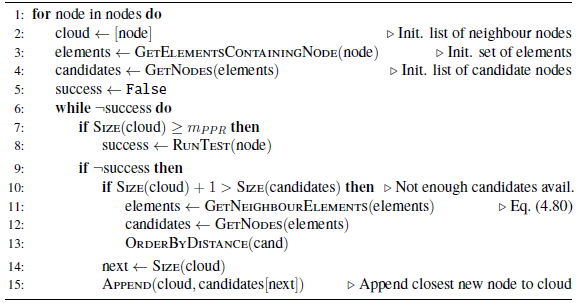
|
|
Algorithm. 4 Creation of clouds (lists) of neighbours (modified algorithm) |
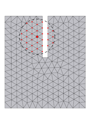
|
| Figure 39: Illustration of the kind of erroneous neighbours cloud that is avoided by taking only nodes from adjacent layers of elements. |
The resulting nodal gradient may then be evaluated at the position of each particle, so that it can be used to calculate the necessary terms in the MRE. In the case of the velocity, it is possible to calculate the full gradient, and then evaluate at the particle position, or else to do so after each component of the gradient is obtained. The second option might be interesting in order to limit the amount of allocated memory by reusing the same container for each component of the gradient.
On the other hand, note that it is possible to avoid repeating the algorithm above every time one does forward coupling by storing the relevant nodal information. Specifically, note that only coefficients , and are needed to calculate the gradient. Therefore only the second, third and fourth rows of the matrix need to be stored for each node. To avoid the search operation at each forward coupling step it would also be necessary to keep a list of the neighbouring nodes, for each node. As we mentioned, the minimum number of neighbours is ten, although it is often necessary to use a larger number of neighbours to avoid ill-conditioned matrices. We have observed the average number of neighbours to be closer to 2.5x101 in practice. Similar numbers have been observed by Ortega [269] in applications of the finite-point method, that employs a similar approach to compute the spatial derivatives. Assuming this list is kept as a list of pointers, one may estimate the total memory requirements to be about 4.4x10² per node. By performing the search at each step this number would fall to about 2.4x10² per node.
This is still a large number that could seriously hamper performance. However, this really depends on the balance between the number of particles and the number of elements to discretize the fluid. If the number of particles is higher than the number of nodes the fluid memory extra requirements will not dramatically affect the overall performance, since the number of variables per particle is often already quite high in practice, especially when using all the terms in the MRE, which requires storing historic information. These memory requirements for the particles become even higher when collisions become relatively common. Nonetheless, this is certainly an important draw-back of the method.
In our code we have implemented the possibility of fixing a maximum number of nodes in a cloud to a predefined number, say, 2x101. The method is then modified to default to the standard method for the nodes where this is not enough. This option makes the method more robust.
Finally, note that the second order polynomial derived allows us to differentiate it twice to obtain the Laplacian directly, where this time the coefficients , and are needed. This requires some extra memory, but avoids the application of the method in succession, as discussed with the previous methods. This was indeed the approach proposed (and analysed) by Guo et al. [153], who obtained interesting results concerning the ultraconvergence of the method in a class of quasi-regular meshes.
The method of Pouliot et al. (FFC)
The method introduced by Pouliot et al. [282] provides an interesting alternative to the PPR. It results from imposing that the recovered nodal gradient must make directional derivatives along all element edges equal to that obtained from the FEM approximation . Note that, while the derivatives are in general discontinuous across elements for piecewise linear elements, the directional derivatives along the edges are in fact continuous.
Let us describe the method. Consider an element edge formed by two nodes and . Once again, assume that the recovered gradient is denoted by . Since it is a linear field, its value at the edge midpoint is given by
|
|
(4.85) |
The directional derivative of along the edge is trivially equal to
|
|
(4.86) |
where is the normalized vector joining to . Therefore, the condition we are seeking can be written as
|
|
(4.87) |
Multiplying booth sides (with the dot product) of Eq.~4.87 by we obtain a system of three equations with six unknowns for the edge (in 3D). But since in the global system there must be three equations per node, we just assign the system to both nodes in the usual assembly process. This can be expressed as saying that the edge contribution to the global matrix is given by the following system:
|
|
(4.88) |
where , and ; and that the assembly is done in the usual way. The assembled global matrix is invertible for most irregular simplex matrices but becomes singular for regular matrices [282], due to the redundancy of a subset of the equations.
In the latter case, instead of adding extra equations to the system, Pouliot et al. propose to stabilize the system. They give two alternatives of how to modify Eq.~4.88 to stabilize the assembled system:
|
|
(4.89) |
where
|
|
(4.90) |
where is the three-by-three identity matrix and is a 'small parameter', that must be made small enough to minimize the error while maintaining the invertibility of the global matrix. Pouliot et al. recommend . Note that the addition of the matrix is equivalent to adding the system , which can be interpreted as requiring that the directional derivatives of the gradient to be all zero along the edges.
The other stabilization option they proposed can be expressed as
|
|
(4.91) |
where are the nodal values obtained by an alternative recovery method. Pouliot et al. proposed to use the method presented in [32], although they accepted the possibility of using other methods, such as the PPR.
This method is attractive for the following reasons. First, it has been shown to be perhaps the most accurate recovery method to date in many cases, surpassing the PPR in most tests reported in [282], who remarked its superiority for approximations near boundaries. Second, it requires virtually no extra memory, since all the data structures needed where already in existence for solving the continuous phase problem. And third, its edge-based approach is fully compatible with the finite element framework, which means that we could automatically take advantage of all the pre-existing tools for the FEM, such as MPI-parallelism etc.
In the following sections the most important alternatives reviewed above are tested. We discuss their adequacy to calculate the derivatives required for a particle-laden simulation code and pick the most suitable ones for the examples that follow.
(1) It is equal to the number of monomials of a polynomial of order in dimension . By a simple combinatorial argument one derives the formula which in our case yields .
4.4.2 Comparison of the different recovery approaches
In order to check the accuracy and robustness of the different alternatives, in this subsection we test the different methods on different example functions and meshes. Here we focus on their performance on cubic meshes, representative of their suitability in bulky domains, where most of the points are far from the boundaries.
Our approach consists in imposing the nodal values to match that of analytic fields and apply the derivative recovery using these nodal values. Since we are mainly interested in the material derivative to calculate , we will measure the error in calculating the convective term . We will also be looking at the error of the recovered Laplacian .
We will consider the following measures of the error:
|
|
(4.92) |
where is the approximated field, its analytical counterpart and where the approximate -norm is defined as
|
|
(4.93) |
We additionally consider the maximum relative error, defined as
|
|
(4.94) |

|
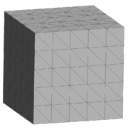
|

|
| (a) irregular mesh | (b) regular, conformal | (c) regular non-conformal |
| Figure 40: Coarsest meshes considered for each of the three families. | ||
We have made a selection of four method combinations for each differential operator. Those are:
- Standard method: Exactly as described in Section 4.4.1. For the Laplacian, we applied the gradient recovery twice to each component, retrieving the trace of the resulting matrix.
- -projection: As described in Section 4.4.1. This technique was applied twice as in item above for the Laplacian.
- lumped -projection: Variation of the method in Section 4.4.1, where directly is projected, using the lumped mass matrix. For the Laplacian, instead, the lumped matrix is used to project the gradient, using it again to obtain the divergence of its diagonal components. This approach is mathematically equivalent to the standard method, as shown in Section 4.4.1, so it serves as a verification test.
- FFC: Method described in Section 4.4.1 with the stabilization from Eq.~4.89. The method was applied twice as in first two items for the Laplacian.
- PPR: Method described in Section 4.4.1 (modified algorithm). The Laplacian was obtained by applying the second derivative to the polynomial fit, as explained at the end of Section 4.4.1; and not by applying the method twice, as proposed in [153].
We have used two analytic fields to compare the different combinations above. Next we present the results for each of the two fields analysed.
Product of sines field
The first field is defined in by
|
|
(4.95) |
where is taken to be equal to .
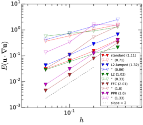
|
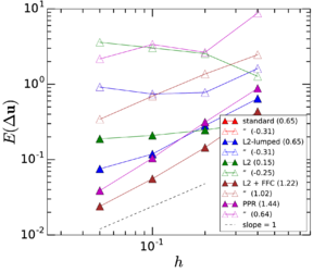
|
(a) irregular mesh |
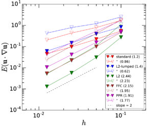
|
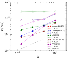
|
(b) regular, conformal |
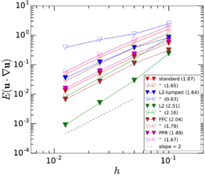
|
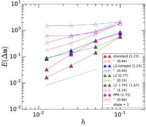
|
(c) regular, non-conformal |
| Figure 41: Recovery errors for the product of sines field, Eq.~4.95 (left column: convective derivative; right column: Laplacian), as a function of the mesh size , normalized by the characteristic scale . Full symbols are used for measure of the error, with the corresponding values in hollow symbols. The obtained order of the different methods, calculated with the two most refined meshes are indicated in parenthesis. | ||
The results of the derivative recoveries are shown in Fig. 41. Both and are shown, the former with full symbols and the latter with hollow symbols. On the left column we find the results corresponding to the convective derivative, for the different types of meshes and, on the right column, the analogous results for the Laplacian.
We will focus on the error as it is more representative of the majority of elements and is clearly much better behaved (more systematic) in all cases. One must however keep in mind that the maximum error is often more than an order of magnitude greater than for most methods, as this can have serious consequences in particle-laden flow simulations. For instance, one must be particularly attentive to the existence of narrow locations, where a large proportion of particles may cross a certain region with a potentially large error in the derivative .
In general terms, the FFC and PPR methods are the only methods that exhibit close to behaviour in the error in most situations for the first-order derivatives, both for regular and irregular meshes. For the irregular meshes, the FFC presents slightly higher convergence rate, at an average for the first column of 2.07 compared to 1.93. Additionally, the FFC presents slightly lower errors for the coarser meshes, which leads to an improvement of around half an order of magnitude when compared to the PPR for the finest meshes. A similar picture is found on right column (Laplacian) where we observe the expected decrease in the order of convergence for both methods, although for both the FFC and PPR methods the order of convergence remains higher than one. These results are coherent with the results presented in [282], which showed a moderate advantage of the FFC method with respect to the PPR.
The general behaviour of the FFC and PPR methods in regular meshes is broadly speaking similar for the convective derivative. Nonetheless, note that for the conformal-type mesh, the FFC shows a stagnation in its convergence rate for the Laplacian. This result is interesting, although compatible in principle with the results from [282], where the second-order derivatives recovery was not discussed. We will come back to this point with the next example field, nonetheless.
About the other methods, focussing on the first column of Fig. 41, it is clear that the standard approach and the lumped -projection approach have similar accuracies for the convective derivatives. The consistent -projection shows comparable accuracy for the irregular mesh but much better accuracy for the regular meshes, where it even surpasses the high-order methods (PPR and FFC), yielding extremely high accuracy, also for .
The second column however shows a different picture: the consistent -projection performs poorly , compared to the standard method and the lumped -projection, which here become identical, as expected, because they are mathematically equivalent in this case (the nonlinearity of the convective term breaks the equivalence for the first-derivatives case).
Ethier field
This fields corresponds to a particular case of a family of analytic solutions of the Navier-Stokes equations found by Ethier and Steinman [121]. These equations are fully three-dimensional and resemble a pair of interlocking vortices.
|
|
(4.96) |
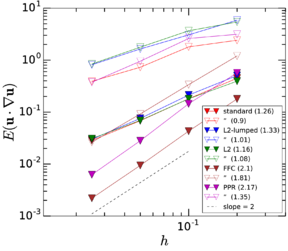
|
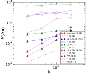
|
(a) irregular mesh |
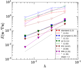
|
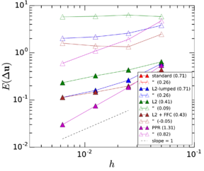
|
(b) regular, conformal |
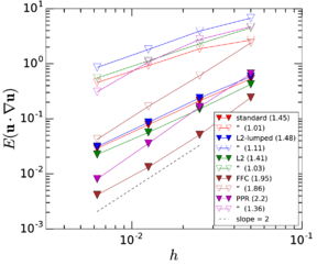
|
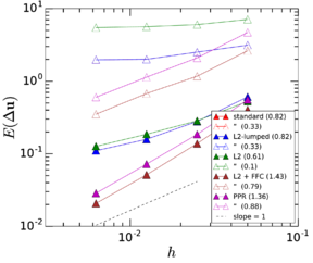
|
(c) regular, non-conformal |
| Figure 42: Recovery errors for the Ethier field at Eq.~4.96 (left column: convective derivative; right column: Laplacian) as a function of the mesh size , normalized by the characteristic scale . Full symbols are used for measure of the error, with the corresponding values in hollow symbols. The obtained order of the different methods, calculated with the two most refined meshes are indicated in parenthesis. | ||
For this field the results are in general worse (larger relative error), as is perhaps to be expected due to the relatively stronger nonlinearities associated to this field. Let us analyse the particular differences observed in Fig. 42 with respect to those in Fig. 41.
For the irregular meshes and the regular, non-conformal meshes the higher-order methods (FFC and PPR) behave similarly, though now the PPR shows a slightly higher rate of convergence. This however does not make up for its lower accuracy for the coarse meshes compared to the FFC.
A more important difference is observed for the regular, conformal mesh. Note that the FFC by far fails to attain its promised second order and becomes much less precise. Note that this loss of accuracy already manifested in the previous example field for the Laplacian. Here, the stagnation is confirmed and takes place both for the convective derivative and the Laplacian.
After very careful scrutiny, we could not find any errors in our implementation. We even compared the explicit matrices obtained for a test example proposed by Dr. Pouliot himself in a private communication, obtaining identical results. Later on, we found that a colleague [105] had run a test on the method by Pouliot, obtaining the desired order. However, we found out that these authors had used non-conformal meshes, which inspired our conjecture that the method is not robust for conformal meshes, precisely the type normally used in finite element simulations. We tried applying small random perturbations to the mesh and the results persisted, suggesting that the problem is related to the connectivity of the matrix.
An additional difference observed is the loss of the ultraconvergent (strictly more than one order over the expected accuracy) character of the -projection method, which moves closer to its expected order-one behaviour [394].
Discussion
We have reviewed several methods as viable alternatives for the derivative recovery operations required in a FEM-based particle-laden simulation code. From the results discussed above we can conclude that
- The standard approach offers a very efficient alternative with attractive properties such as small radius of influence (it does not require a large patch to work) and a predictable and robust behaviour that often exceeds the expected first-order behaviour for the convective derivative.
- the standard approach is not as accurate and robust for the calculation of the Laplacian, for which a higher-order method would be recommended
- The method of Pouliot et al. (FFC) is a very accurate method, perhaps the most accurate method when it works. This is especially true for irregular meshes, for which it shows very good properties, as previously found in the literature.
- However, the FFC suffers from low accuracy for some types of regular meshes, even when stabilized according to the original formulation. More work is needed to fully understand the origin of this issue, but we regard it as unsafe until it can be fully fixed.
- The method of Zhang and Naga (PPR) is accurate and robust in all situations. Its main drawback is its high memory requirements, as it is a patch method that only requires a moderate number of multiplications per node.
We therefore adopt as a default strategy the PPR with the standard approach fall-back for failed polynomial fits. When the number of unknowns is very big, we simply stick to the standard approach though acknowledging its lower accuracy.
Finally, we come to the conclusion that an accurate calculation of the Laplacian would probably require higher-order FEM methods in the first place, unless an extremely fine mesh is used. Fortunately, there are many situations were the Faxén terms can be neglected and we will therefore not consider these corrections in the forthcoming sections.
4.5 Forward coupling
Once the continuum phase solution has been determined (including the recovered derivatives) there must exist an interpolation process to update the information at the particles' locations (their centres), as they will in general fall at arbitrary, intermediate, positions within the domain 1. This process generally consists in the following steps
- Locate the relevant computational cells for each particle
- Calculate values from the cells
Let us next discuss each of these.
(1) Unless the particles' locations are used as computational points, see for instance [67]
4.5.1 Search
For a given particle, the data that is needed to reconstruct the flow at its center is usually only a small subset of the total available information: that related to a neighbourhood of the point in question. Since the brute-force survey of all the discrete information (for each particle) is out of the question, it is necessary to implement a suitable search algorithm to relate each particle with the relevant data in an efficient way.
Our algorithm is based on the same technology used for the inter-particle search. Taking advantage of the abstract syntax offered by Kratos, we create a bin data structure [369] that pre-classifies objects, in this case tetrahedra, so that the search of the host element for points can be achieved then in constant time. Since we are dealing with constant fluid meshes here (except when using an ALE method, see Section 4.7), there is no need to update this bin data base and it can be reused at every time step.
The search can be further optimized by using the fact that particles cannot jump several elements between time steps, see [215]. In our examples, we have not found the search related to the coupling to ever dominate other costs and thus we have not implemented such methods. Nonetheless, this is an interesting topic for future research.
4.5.2 Interpolation
For some methods, such finite volumes or finite differences, the solution is a discrete set of values associated with a discrete set of spatial points. Since the position of the particle will surely not coincide with any of these points, the information must be interpolated, incurring in an additional error that should be taken into account. Consequently, the approximation order of the interpolation scheme is usually taken to be of the same order as the numerical method's own [11,62]. Sometimes it is taken higher [236]. The goal is to preserve the order of accuracy of the velocity once transferred to the particle.
In other cases, such as in the FEM, the approximated solution is defined in the totality of the domain and it is a matter of simply calculating the needed values at particular positions. For instance, we use linear tetrahedra, for which the velocity at the location of a given particle, labelled , is calculated as
|
|
(4.97) |
for and for taking values from the set of four global indices corresponding to the four nodes of the tetrahedron that contains the particle , which is known thanks to the search algorithm. and similarly one could interpolate the velocity gradient if the nodal values were known. This operation entails no further errors apart from those associated to finite-precision arithmetic.
On the other hand, even when the approximate solution is defined everywhere, there might be reasons to employ interpolation instead. For instance, with pseudo-spectral methods interpolation (using the coefficients of the shape functions as the discrete values) is preferred over evaluation because of the large computational cost of the latter [20]. Note that in fact in this case the order of approximation is often lower than that of the solution (spectral methods can achieve exponential approximation order under optimal conditions). In practice however, this error can be made sufficiently small by considering high-order polynomials, see [20]. See also [354,351] for a recent and detailed review of several interpolation schemes used for particle-laden flow simulations with pseudo-spectral methods for regular grids. In any case, the interpolation order is not recommended to be lower than third-order ( behaviour of the error) to obtain very accurate results [377,330] in the context of DNS using PS methods. Note that this reinforces the notion that it is important to strive for achieving at least this accuracy in the derivative recovery.
There is a temporal discretization associated to forward coupling. This is because it is common to have a different time stepping scheme for the particles and for the fluid, since these two phases have different smallest characteristic scales. We employ an updated-fluid strategy, by which the fluid is updated first, and then the particles motion is integrated until they meet the fluid, in one or (typically) more sub-steps. As the particles change location during these sub-steps, we use a linear interpolation of the past and present values of the fluid, interpolated at the present location of the particles. For the case of pre-calculated fluid, where the fluid has been previously calculated and stored and the particles are moved with the read fluid data, it would be possible to use higher-order temporal schemes, as the fluid at all time steps is known. Such schemes would become particularly relevant for higher Stokes numbers and less so for small Stokes numbers, as the quasi-stationarity becomes a better and better model for the fluid motion, as seen by the particles, between successive fluid time steps. We have not pursued this here, and we leave the study of such schemes for future works
4.6 Application example: T-junction bubble trapping
We report in this section a first application example to test the coupled DEM-CFD approach, where the fluid is calculated using linear finite elements and a one-way strategy is used to move the particles according to an extended version of MRE for higher Reynolds numbers. The problem is taken from [356], where it was studied both experimentally and numerically, using finite-volume based commercial software.
The system consists in a T-type tube junction through which a steady water flux is imposed (see Fig. 43a). The flow is laden at the entry with a number of bubbles, which are idealized as spheric, rigid particles (empty glass spheres were also used in part of the experiments). The phenomenon to be studied here is the bubble trapping that was observed to occur around the junction point for a remarkably wide range of parameters.
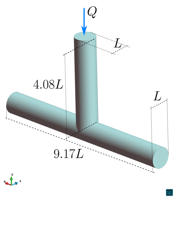
|
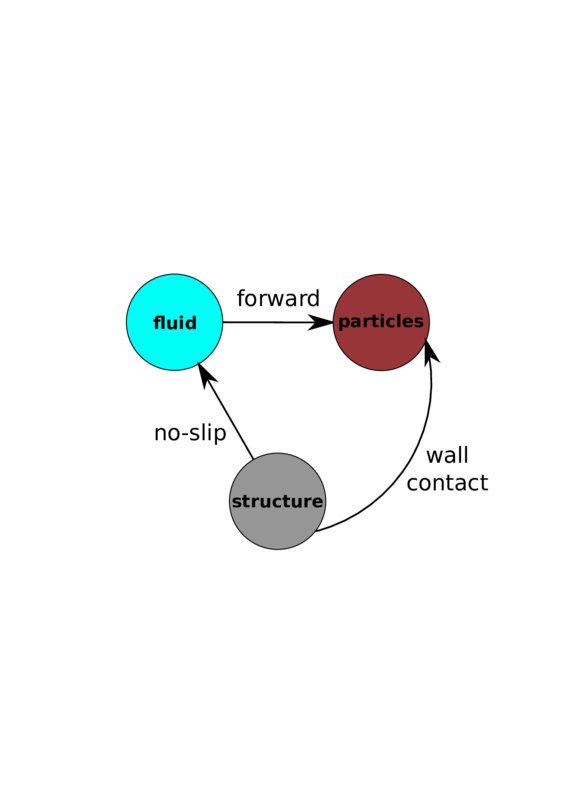
|
| (a) Geometry of the T-junction considered, with characteristic dimensions. The inflow flux is indicated with a blue arrow. | (b) Conceptual diagram of interactions taken into account in the t-junction example; to be compared to Fig. 38. |
| Figure 43 | |
4.6.1 Flow simulation
Our goal is to run a fluid flow simulation that is sufficiently accurate for a sufficiently long time to give a realistic representation of the real flow. The flow solution (the nodal values of the velocity field) is stored in a n HDF5 format file [341] and read afterwords, post-processed and used to integrate the particles positions. The advantage of this strategy is that many particle simulations can be run with the same flow. In this case the flow simulation was clearly the most expensive part, given that the numbers of particles required were moderate and that the particles could be modelled as relatively soft spheres.
The flow data is read from a file, but the derivatives are recovered during the particles simulations. This is acceptable, as the derivative recovery is much less costly than solving the fluid system. In this way we were able to keep the size of the fluid post-process files manageable.
Inputs
The boundary conditions were set to no-slip on the tube walls, uniform velocity at the inlet and constant and equal pressure at the two outlets. Gravity was neglected as in [356].
| Parameter | Value | Description |
| Fluid parameters | ||
| 1x10³ kg m-1 ^3 | density of fluid | |
| 1x10⁻³ s m-1 ^2 | kinematic viscosity | |
| Particles parameters | ||
| 1.5x10² kg m-1 ^3 | density of bubbles | |
| COR | 2x10⁻¹ | coefficient of normal restitution |
The particles are represented by spheres whose motion is calculated according to the soft-sphere discrete element model described in Appendix A. The particles are introduced in the domain through an inlet surface, which is a flat triangular mesh where the nodes are the inception location of the particles. The initial velocity of the particles is set to be equal to the average flow velocity, so that a small relative velocity is present from the beginning. This initial slip velocity is given enough time to dissipate though, by the time the particles reach the t-junction through the action of the hydrodynamic interaction forces. The principal particle parameters are summarized in Table 8. The coefficient of normal restitution (COR) is the ratio between the incident impact velocity and the reflected impact velocity, such that the proportion of kinetic energy remaining after the impact is roughly given by for direct impacts. For air bubbles in water it is related to the Stokes number of the bounce, which can be estimated as [386]
|
|
(4.98) |
where can be (safely, since we want to show it is small) estimated as , the characteristic scale of the flow. Substituting in the biggest sizes considered for the particles () and Reynolds numbers we obtain , for which it is realistic to take ; see [386].
The stiffness of the sphere was set to 1x10² Pa , which was calculated to avoid excessive indentations during the simulation. Particle-surface contacts are not prevalent in any case and do not influence the motion of the particles significantly. However, it is advantageous to have a soft contact, as it allows taking larger time steps for the integration of the trajectories.
Hydrodynamic model
To model the motion of the particles we will start by using the same hydrodynamic model proposed in [356], which is a simplified version of Eqs. 4.1 and 4.4, where it is assumed that and the model of Schiller and Naumann (1935) accurate for (see [222]), is used for the drag coefficient
|
|
(4.99) |
For these authors use the formulation based on the pressure gradient and the divergence of the deviator stress tensor, equivalent to our formulation in the continuum limit. The equivalence is obtained by expressing in terms of the stress tensor using the Navier–Stokes equations:
|
|
(4.100) |
where the weight is neglected in this case, following the criterion in [356], where it is argued that. Note that the data in Table 8 lead to ; and , which casts some doubt on the validity of such assumption. We will nonetheless keep this assumption to simplify the discussion.
Furthermore, the deviator stress tensor contributions are deemed small in [356] and neglected. This is a common practice that is nonetheless unnecessary if one uses the alternative formulation based on the material derivative, although the latter practice does require two more derivative recoveries (we must recover the convective derivative instead of just the gradient of the pressure), plus an additional time derivative. We thus keep this term, as we are using the formulation based on the material derivative.
Finally, no rotational degrees of freedom are considered. In this system the rotational velocity of the particles is not expected to vary greatly from half the local fluid vorticity. This can be justified based on the very small rotational Stokes number, , based on Eq.~2.23 and the data in Table 8. Such small value implies that the bubbles angular velocity relaxes very rapidly to that of their surrounding fluid. Eq.~2.23 is strictly valid only under the small particle Reynolds number hypothesis, but here it should be sufficiently accurate to provide an order-of-magnitude estimate.
| Parameter | Value | Description |
| 3.6204x10⁴ | total number of particles injected | |
| 4.68x10⁻¹ | maximum value attained by | |
| 3.142x101 | dimensionless final time | |
| 2.6x101 | dimensionless max. injection time considered in statistics |
4.6.2 Trapping probability
We attempt to reproduce in this paragraph a numerical result presented in [356], where the proportion of particles that become trapped is measured, for a fixed and several particle sizes. In order to do this, we run the simulation for a total time that exceeds the characteristic time scale about thirty times, see Table 9. A fixed flux of particles is imposed using the inlet mesh depicted in Fig. 45a, which provides a sufficiently fine discretization of the whole cross-section. The particles are considered trapped when they remain inside the control volume , which is the parallelepiped comprised between two cross-sections located at opposite sides of the junction, at a distance of from the plane of symmetry. Then the proportion of particles trapped is computed as
|
|
(4.101) |
where represents the proportion of particles trapped, is the total number of particles injected before time and is the number of these particles present by the end of the simulation inside the control volume that where injected before time (i.e.newer particles are not counted). The results shown in Fig. 45b correspond to the numerical predictions for for several particles' radii; where is the distance from the geometry's plane of symmetry at which the particles are injected, normalized by .
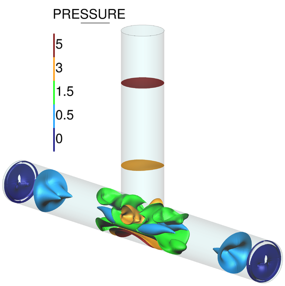
|
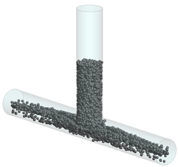
|
| (a) Pressure isosurfaces at nondimensional time . | (b) Snapshot of non-interacting particles at (about 2x10⁴ particles). |
| Figure 46 | |
4.6.3 Discussion
We have applied our CFD-DEM strategy to simulate the phenomenon of bubble trapping in T-shaped junctions. We used a one-way strategy that was sufficient to reproduce the trapping and to obtain a qualitative picture similar to that obtained in the earlier work of Vigolo et al. [356].
Our results confirm that the overall approach can be used for the detection of bubble trapping in T-junction systems and other, similar, moderate- systems. The one-way coupling strategy allows the application of an efficient methodology, whereby a good fluid simulation is only run once, while a large number of cases with particles can be run at a reduced cost by reading the pre-computed results. The derivative recovery may or may not be calculated during the fluid solution, allowing for extra freedom in later simulations. The elimination of inter-particle interactions allows to further speed up the simulations, since it is possible to use an artificially increasing number of particles at a time, decreasing the total simulation time required to reach statistical significance.
Our numerical results do present difference with respect to the ones presented in [356] were the trapping probability was observed to be (quite consistently) higher for all the radii. Furthermore, their predicted maximum trapping was found to be closer to , whereas our prediction is closer to . The difference persisted even as we refined our mesh and so there remains some uncertainty regarding the accuracy of the method that should be further tested, perhaps against physical experiments or fully-resolved simulations; despite the high computational cost associated to the latter.
We can identify a number of factors that could explain the observed differences. The most obvious difference is that our formulation includes the deviator stress tensor term (first term of the RHS of Eq.~4.100) implicitly, while it was neglected in [356] as it was deemed small. But in fact, a simple scaling analysis confirms this hypothesis, since (using )
|
|
(4.102) |
as the Reynolds number is close to 4x10². Note that in Eq.~4.102 we have assumed that the material derivative is of the same order as the convective derivative.
Another possibility is the existence of differences in the accuracies of flow solution itself, which could exist between the two works, including the derivative recovery. This is difficult to test though, since the detailed flow information is not available for comparison. More work is needed to produce robust guidelines for the application of our CFD approach safely; including mesh tolerances and convergence criteria for the velocities and for their derivatives.
Other possible sources of differences inclstokes dragude the time integration of the particles trajectories (although we have proved the accuracy of our algorithm extensively in Chapter 3) and differences in the initial injection positions (it is not detailed in [356]), the level of statistical convergence (the number of particles is not given either).
Finally, the influence of other neglected effects requires further study, especially if precise quantitative predictions are the goal, such as
- the effect of the history force
- the inter-particle effects (three and four-way coupling)
- the influence of the Faxén terms
We have nonetheless run a simulation to check the magnitude of the effects of including the history force. A slip velocity estimate based on a similar argument as that used in 2.89, but this time using the drag force formulation in Eq.~4.99. Doing this and solving for the slip velocity we obtain for all the radii studied, which results in , for which the Basset–Boussinesq history model can be safely applied. In case higher particle Reynolds numbers had occurred, the approximate method by [108] could have been used instead (without major modifications of the algorithm described in Chapter 3), which showed good predictions in the range . The results shown in Fig. 47 indicate that the effects might not be negligible in this range, and so it is probably preferable to include the effect in cases where accurate quantitative results are required.
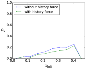
|
| Figure 47: Trapping probability for as function of , comparing the results with and without the effect of the history force. |
4.7 Application example: Particle impact drilling
In this section we use a one-way coupled strategy to analyse an engineering system that has been studied very little either with numerical methods or experimentally: the particle impact drilling (PID) method. Among the scarce exceptions we find the numerical works [87,185,289], all based on finite volume method, and the experimental work [375], that studied the rate of erosion of the substrate under different impact conditions.
This drilling technology is used in the oil and gas industries to achieve greater rates of penetration than the traditional alternatives. In its basic features, a PID drill-bit is similar to a conventional one: it consists of a cutter fixed at the end of a rotating tube through which the drilling mud is pumped from the surface. The bit has apertures that allow the mud to flow out of its tip, cleaning the cuttings and dragging them back to the surface through the annulus contained between the outer surface of the tube and the hole’s casing. A PID system is unique in that the mud flow is laden at the surface with small steel balls to help erode the rock and increase the rate of penetration. When the balls reach the tip of the drill-bit, they are violently accelerated as they pass through any of the particularly narrow apertures (nozzles) at the tip of the drill bit, where they acquire the necessary kinetic energy to effectively erode off material from the rocky bed. Inside the nozzles the fluid can attain velocities in excess of 2x10². A schematic diagram of the workings of the system is shown in Fig. 48a.
Our coupling strategy is represented by the diagram in Fig. 48b. We include two new types of interactions with respect to Section 4.6: the inter-particle interactions, as it has been observed that they have a strong influence in the particles' flow, and a particle-to-structure interaction in the form of a qualitative wear. This is a measure of the strength and frequency of the particles' impacts on the solid surfaces and it has been considered as an interaction, although is really only a matter of post-processing and dues not couple the solid solution with that of the particles. This type of interaction could also be seen as a trivial or degenerate type of interaction.

|
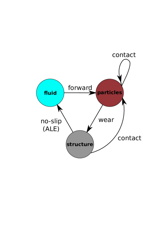
|
| (a) Diagram of workings of the PID wellbore, showing inflow mud with steel particles, and up-flow cuttings wash-up. | (b) Conceptual diagram of interactions taken into account in the PID example; to be compared to Fig. 38. |
| Figure 48 | |
4.7.1 Problem data
The work related to the present application example was done under the terms of a private consultancy contract with a consultancy firm that also provided the geometry and input parameters.
Domain geometry
The geometry of the drill-bit and the surfaces defining the rocky bed and casing are shown in Fig. 49. The surfaces in red belong to the rotating part of the domain, while the casing and ground surfaces are shown in a transparent blue. The inlet surface, at which the inlet flow condition is imposed is marked yellow, while the outlet surface (imposed normal traction) is marked in light green. In Table 10 we summarize several useful measurements derived from the geometry.
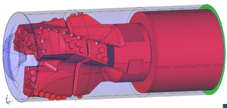
| |
| bottom-up view | |
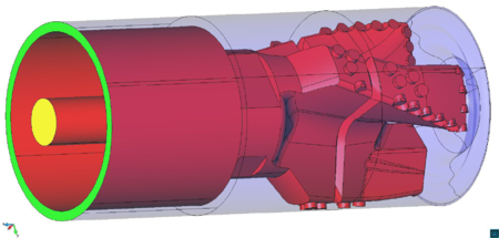
| |
| top-down view | |
| Figure 49: Depiction of the domain geometry. | |
| Parameter | Value | Description |
| 5.3975x10⁻² m | interior diameter of inner tube | |
| 7.69x10⁻³ m | interior diameter of nozzles | |
| 8.6x10⁻² m | average length of the nozzles | |
| 1.11x10⁻² m ^3 | total fluid domain considered | |
| 1.53x10⁻³ m ^3 | fluid of internal domain (between inlet surface and tip of nozzles) |
Parameters
The values that have been kept fixed throughout this study are summarized in Table 11.
| Parameter | Value | Description |
| Fluid parameters | ||
| 1.294x10³ kg m-1 ^3 | density of fluid | |
| 7.61x10⁻¹ | flow behaviour index | |
| 1.24 Pa s ^0.761 | flow consistency index | |
| Particles parameters | ||
| 1.9812x10⁻³ m | diameter of steel particles | |
| 7.85x10³ kg m-1 ^3 | density of steel particles | |
| Operation conditions | ||
| 2.902x10⁻² m ^3s-1 | fluid flux | |
| 1.5x10⁵ s-1 | number of particles flux | |
| -2 s-1 | angular velocity of drill-bit | |
4.7.2 Drilling fluid model
The typical drilling mud used in the oil and gas industries has a non-Newtonian behaviour. This means that its motion is not well-approximated by the standard Navier-Stokes equations, which must be modified. A common type of model used in this context is the Herschel–Bulkley fluid [214]. This type of fluid departs from the Newtonian behaviour in two fundamental aspects:
- The fluid has a finite yield stress, which is a threshold below which no flow takes place and the fluid behaves essentially as a solid.
- For shear stresses larger than the yield stress, the viscosity changes with the shear rate.
The constitutive equation for this type of fluids is commonly written as a generalized Newtonian fluid by replacing the constant viscosity by the effective viscosity, as a function of the flow:
|
|
(4.103) |
where is the local strain rate, given by
|
|
(4.104) |
where
|
|
(4.105) |
In Herschel–Bulkley fluid the functional dependence of the effective viscosity on the strain rate reads
|
|
(4.106) |
where is such that there is continuity at . The material parameters and are known as the flow consistency index and the behaviour index respectively. One distinguishes between shear thinning fluids () and shear thickening fluids (). The fluid becomes less viscous with increases of the shear rate in the former, while the opposite is true for the latter. Drilling muds are all of the shear thinning type [214].
We are particularly interested in the special case where , that defines the family of power-law fluids, whose qualitative behaviour, both for shear-thinning and shear-thickening fluids, is shown in Fig. 50. It is quite common to have drilling muds described by this model. Moreover, it was required by the consultancy firm that the flow should be modelled as a power-law fluid.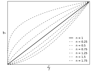
|
| Figure 50: Strain rate-stress relation for a power-law type fluid undergoing pure strain at a constant rate, for different flow behaviour indices ( corresponding to a Newtonian fluid). |
The continuous problem associated to the fluid phase consists in the generalized Navier–Stokes equations, given by:
|
where is the effective viscosity, encoding the non-Newtonian behaviour of the fluid. In order to have a well posed problem, we need a set of initial and boundary conditions of Dirichlet and Neumann type as given in Eq.~4.15.a.
4.7.3 Hydrodynamic interactions for the particles
Here we again consider a hydrodynamic model of the form of the simplified Eqs.~4.1 and 4.4, where it is assumed that . Regarding the viscous forces (), the particular expression that we have used is described in Section 4.7.3.
To the best of our knowledge, no empirical expressions exist for the history term in non-Newtonian fluids and finite Reynolds number. Given the uncertainties involved and its secondary importance for flows with reasonably high Stokes numbers, we have neglected it.
The importance of the lift force is often secondary as compared to the steady drag force, although in some cases it can become important [219]. Nonetheless, we have neglected its influence in the present work, although we acknowledge its potentially significant importance and further investigation of this issue, including the study of suitable formulations is left for future work.
Finally, no hydrodynamic torque has been considered for the rotational degrees of freedom. Here too, we have opted to keep the formulation simple and so we also leave its consideration, along with that of the lift force, for future work.
Non-Newtonian Drag
In order to obtain an appropriate equation of motion in the non-Newtonian setting, we make the assumption that the same additive superposition of the different forces discussed in Section 4.2 is still applicable in this setting. Other authors have made the same assumption [3]. Furthermore, since the non-Newtonian effects are captured by a varying viscosity, we will assume that the unperturbed flow and added mass forces, which are independent of the viscosity for Newtonian fluids remain unchanged, since all the non-Newtonian effects are concentrated in the varying viscosity. Having neglected the effect of the lift force, it is therefore only left to determine a steady drag law.
The literature on the hydrodynamic forces of a sphere submerged in a non-Newtonian fluid is certainly much more scarce than that for Newtonian fluids. A comprehensive review can be found in [16]. Nonetheless, here we employ the empirical expression proposed by Shah et al. [312] to predict the terminal velocity of particles in power-law fluids in the context of drilling operations. Their formulation has only been tested in stationary conditions but due to our hypothesis of the additive decomposition of the different effects, we will consider it adequate for our purposes. They provide the following expression for the empirical drag coefficient
|
|
(4.108) |
with the empirically determined parameters
|
|
(4.109) |
and where the particle Reynolds number is defined as
|
|
(4.110) |
The model above is valid for and . Note that using the characteristic values calculated in Section 4.7.4 we can check whether the conditions for the validity of this model are met. The value of is clearly well into the range of validity. In order to estimate the characteristic values of we can use the estimates for the mean velocity and assume a conservative value for the relative velocity based on it, say 5x101 of its value. For instance, in the inlet tube area, this estimate would yield , while this number could reach inside the nozzles. Again, it is expected that the maximum relative velocity occurs inside the nozzles and since the value of is estimated to be only slightly greater than the range of validity there, we will accept the associated error nonetheless. The error associated with this choice is unknown but we do not expect it to be too large, especially when taking into account the low degree of non-Newtonian behaviour ( relatively close to one) of the mud.
Final model for the hydrodynamic interactions
Summarizing, we will consider the following the equation of motion for an isolated particle, suspended in the drilling mud:
|
|
(4.111) |
where the binary parameter is introduced to easily turn off the pressure-related terms as required.
Summary of limitations of the model adopted
The models adopted for the description of the hydrodynamic interactions inevitably contain a number of assumptions and simplifications that contribute to the final error in the simulations. We next list the most important of these factors. Some of them can be addressed by further developments that will be discussed in Section 5.2.5.
- The drag model is used slightly out of its range of applicability inside the nozzles, which could impact the calculated impact velocity. Furthermore, this drag is based on empirical data looking at terminal velocity data, rather than complex dynamics.
- The lift force has been neglected altogether for simplicity. However, this is not well justified and further work on this issue is needed.
- Similarly, no hydrodynamic torque has been taken into account. Its influence is expected to be rather weak, though, especially when no Magnus effect has been considered (it only affects impacts).
- The additive property of the different effects in the equation of motion requires further testing. However, the same assumption has been made by many authors based on extrapolations and partial evidence in the Newtonian fluid setting.
4.7.4 Characteristic scales of the problem
In order to verify the range of applicability of the different models and the level of numerical resolution required for the simulations it is important to survey the different scales involved in the problem. Let us thus examine them
Characteristic scales of the flow
Let us start by considering some characteristic scales relevant to the continuous problem. From Tables 10 and 11, one can estimate the average velocities in the different sections of the geometry. Similarly, the fluid residence time (average time spent by the fluid molecules in the domain) can be calculated by dividing the volume over the flux. These and other derived quantities relevant to the fluid are included in Table 12.
A Reynolds number can be calculated for power-law fluids, following Metzner and Reed [247], as:
|
|
(4.112) |
who also experimentally derived the following criterion for the transition to turbulent flow:
|
|
(4.113) |
Note that, according to the estimates discussed above the flow in the inner inlet tube is expected to be just on the verge of turbulence () and only moderately turbulent in the nozzles ( assuming equal distribution of flow among the four nozzles). Note that this is the maximum Reynolds number expected in the flow, as this is the most constrained section of the conduct and
|
|
(4.114) |
which is monotonically decreasing. We thus expect a mostly laminar or transitional flow regime, with some areas presenting weak turbulent or transitional regimes. Relatively moderate turbulence is expected inside the nozzles.
With regards to the near-boundary resolution, one can calculate an analogue to the distance by Trinh [346]
|
|
(4.115) |
where is the shear stress at the wall, which can be estimated as
|
|
(4.116) |
and where is the friction factor [247]. It is interesting to calculate the distance from the wall, , at which , since that is the size recommended for the smallest computational cells placed close to it [214]. These values are summarized in Table 12.
| Parameter | Value | Description |
| Flow | ||
| 1.268x101 m s-1 | average velocity in inlet tube | |
| 1.562x10² m s-1 | average velocity in nozzles | |
| 3.8x10⁻¹ s | total domain residence time | |
| 5.3x10⁻² s | internal domain residence time | |
| 2.8x10⁻⁴ m | recommended size of computational cell adjacent to the wall (inlet tube) | |
| 1.8x10⁻⁵ m | recommended size computational cell adjacent to the wall (nozzles) | |
| Particles parameters | ||
| 1.9812x10⁻³ m | diameter of steel particles | |
| 7.85x10³ kg m-1 ^3 | density of steel particles | |
| Mixed parameters | ||
| 2.1x10⁻² | solid volume fraction | |
| 1.28x10⁻¹ | solid mass fraction | |
| Operation conditions | ||
| 2.902x10⁻² m ^3s-1 | fluid flux | |
| 1.5x10⁵ s-1 | number of particles flux | |
| -2 s-1 | angular velocity of drill-bit | |
Characteristic scales of the particles
Stokes number The Stokes number is defined as the quotient between the particle's relaxation time and the typical time scale of the background flow fluctuations, as in Eq.~2.4. We have seen in Chapter 2 that when the assumption of Newtonian fluid and creeping flow is valid (very small ), this relaxation time is a constant. This definition is still applicable in the context of power-law fluids, although its expression here is dependent on a variable viscosity, which complicates its analytic determination.
In Fig. 51 the relaxation times for the steel particles are shown as numerically calculated for different initial relative velocities. The range of values covers all the values of interest in the domain and however the relaxation time is seen to remain quite stable around 3x10⁻³ s . This time scale can thus be used as a reference relaxation time in what follows.
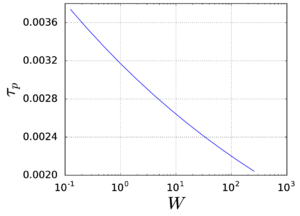
|
| Figure 51: Relaxation times for different initial relative velocities obtained numerically using the drag model of Shah, see Section 4.7.3. |
The Stokes number can be used to distinguish particulate flow regimes, classifying them into ballistic () and tracer-like () with respect to the fluid motion associated with the time scale . When is much greater than one, it is normally assumed that the particles do not have time to respond to the fluid dynamics, see for example the discussion in [19]. In order to estimate the importance of an accurate description of the turbulent structures, it is therefore useful to look at the Stokes number.
For instance, we have seen that inside the nozzles we expect to find the most intense turbulence. But since the particles move at about 1x10² m s-1 there, they only spend less than 1x10⁻³ s in them. This means that and most likely , as the typical turbulent fluctuations will be significantly smaller spacial amplitude than the length of the nozzles. This means that it is mostly the mean flow that will dictate the trajectory of the particles inside the nozzles. Note however that this is true as long as the drag force is the/a dominating hydrodynamic force. We will come back to this question in Section 4.7.8.
Characteristic scales related to the interactions
In order to assess the importance of the influence of the particle in the flow, the most important scale is the typical solid fraction, which is the global proportion of particles volume to fluid volume [85]; see also Section 4.8.4. Another interesting quantity is the solid mass fraction that takes into account the different densities of the two phases. These quantities can be preliminarily estimated assuming a homogeneous distribution of particles as
|
|
(4.117) |
where is the volume of one steel ball. The characteristic values for the present problem can be found in 12.
4.7.5 Discussion of the coupling strategy
Forward FSI interactions
The coupling between the fluid phase and the solid phase is given by the imposition of the no-slip condition at the walls. In this case, we have opted for an arbitrary Lagrangian-Eulerian (ALE) formulation [106] with a moving mesh that moves jointly with the drill bit. In this case the mesh velocity is known exactly and coincides with the rotating velocity of the bit.
Forward Hydrodynamic interactions
The fluid velocity field values are determined at the center of each particle using the linear tetrahedral shape functions of the FEM mesh. The derivative recovery tool of choice was the standard method. We chose this method based on two considerations:
- The large size of the systems to be studied, which meant that it became unmanageable to use the PPR method for the available memory.
- The existence of very narrow sections, for which it was feared that the larger size of the element patches needed for the recovery lead to inaccuracies in these thin regions, for which the number of elements is limited.
Backward FSI interactions
Neglecting the backward action of the fluid on the structure, the backward fluid-solid interaction (FSI), is reasonable, based on the near-homogeneity of the mass distribution inside the drill-bit and the stiffness of the structure at the pipe-length scales of study.
Inter-particle hydrodynamic interactions
The inter-particle interactions are associated with the fluid field disturbances caused by the presence of nearby particles. Such disturbances are responsible for phenomena such as drag reduction due to the wake effect, which can become important at short distances. Such effects are difficult to take into account due to their dependence on the details of the particles spatial configuration, and only approximated relations such as empirically modified drag coefficients are available at particle Reynolds numbers greater than one; see, e.g. [31]. To our knowledge, there is no expression available in the literature for non-Newtonian fluids, and studying the possibility of adapting formulations derived in the Newtonian setting is left for future work.
The error introduced by this effect is negligible when the inter-particle distance grows substantially above the diameter. In [216] five is suggested as the number of diameters, which leads to a maximum solid volume fraction of . Since we are about five time above this threshold we should expect a significant error, especially wherever particle agglomeration or clustering takes place, although it is not easy to quantify. Qualitatively, the expected results would be overall increased ejection velocities due to the lack of a wake effect.
Backward coupling with the particles
We distinguish between two types of effects of the particles on the fluid phase. The first is associated to the momentum transfer between phases, while the second is related to the conservation of mass. Both effects can be taken into account within the point-particle approach, although we have left their inclusion to future work. Next we discuss each of the effects separately.
Force coupling The hydrodynamics forces that the fluid exerts on the particle are, by Newton's Third Law, the forces that the particles exert on the fluid but with the opposite sign. The importance of these forces on the macroscopic flow (which then in turn is used to move the particles) is negligible if the concentration of particles is small enough. In [216] the criterion for negligible influence is suggested. At , see Table 12, it is possible that neglecting this effect can introduce a significant error, but we do not expect it to be critical, since unless there are very large inhomogeneities in the flow (especially in the transverse direction), the streamlines should not be greatly affected. This means that although the pressure drop might not be well captured, the fluid velocity will, leading to a fairly reasonable prediction of the particles' movement.
Mass conservation effects The mass conservation equation Eq.~4.14.b does not take into account the volume displaced by the particles. This simplification would not be expected to lead to very large errors if the expected average value of , see Table 12, remained reasonably uniform (the flow through a regular lattice of particles with the same volume fraction would essentially just be sped up by 2 ). However, some degree of nonuniform particle agglomeration in some regions of the domain is expected. In these regions, the error could become important. The region inside the nozzles is particularly sensitive to this effect due to their thinness. We will come back to this issue in Section 4.7.8; see also Section 5.2.5. Note however that, at least to some extent, the error introduced by this simplification cancels out with the error described in Section 4.7.5, since this simplification leads to a underestimation of the real velocity (wherever there is particles accumulation), while the drag force is overestimated due to neglecting the wake effect, as we have seen.
4.7.6 Final algorithm
Given that the DEM phase has a much stricter time step requirements than the fluid, due to the very small time scales associated to the contact dynamics that it resolves, we employ a sub-stepping scheme so that, for every fluid time step, many DEM time steps are performed. The fluid is advanced first, and then the DEM catches up in smaller time step increments. The fluid field quantities are evaluated at every DEM step too taking a weighted average between old and new fluid values. The pseudo-code is shown in Algorithm 5, where refers to the total number of fluid time steps in the simulation and where keeps track of the time for the DEM phase.
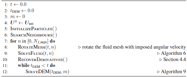
|
|
Algorithm. 5 One-way coupled two-phase algorithm. |

|
|
Algorithm. 6 SolveFluid function algorithm. These operations are performed at every fluid time step. |
4.7.7 Time and space resolution
In this section we present the level of discretization that we use for the description of the fluid and the particles.
Discretization of the particles phase: time step selection
The determination of the time step for the DEM must ensure that the maximum indentations that occur during the simulation avoid unrealistic particle positions, such as particles squeezing through too-narrow passages or even traversing solid boundaries. Furthermore, the numerical stability of the explicit time-integration scheme must be ensured. Finally, the contact duration must be resolved with enough time steps to avoid excessive inaccuracies, taking into account the large uncertainties associated with particle rebounds. To avoid risky iterations (each simulation requires a significant amount of time) we used the methodology explained in Section 6.2.1. The values involved in this process for the two basic cases are summarized in Table 13. Note that they are not the same for the total case (which includes the impacts of the particles on the bed) and the internal case, which only presents very skewed impacts as it does not include the bed area.
| Parameter | Internal flow | Total flow |
| number of subdivisions of shortest contact | 2x101 | 2x101 |
| security factor | 3.25x10⁻¹ | 3.25x10⁻¹ |
| maximum expected normal impact velocity | 8x101 m s-1 | 2x10² m s-1 |
| 5x10⁻⁷ s | 1.9x10⁻⁷ s |
Discretization of the fluid phase: mesh selection
In order to estimate the mesh sizes required for the simulations we run a mesh convergence study based on a single nozzle. The nozzle was attached to an idealized cylindrical structure to which an inlet velocity boundary condition was imposed so as to match the expected flux.
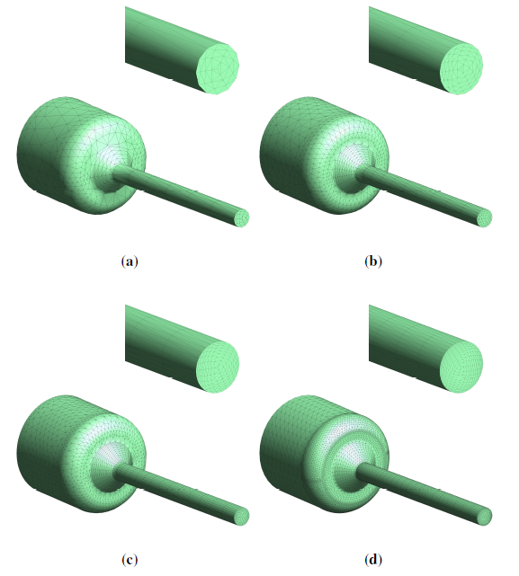
| |
| Figure 52: Meshes used in the mesh-convergence study. From coarsest to finest, approximate number of elements: 5x10³, 1.6x10⁴, 4.8x10⁴, 2x10⁵. The inserts show a zoom into the tip of the nozzles. | |
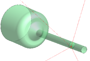
|
| Figure 53: Point of measure of the velocities. |
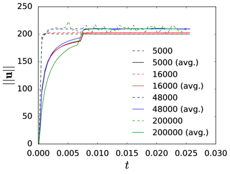
|
| Figure 54: Mesh convergence study. Velocity evolution of a point at mid-shaft, mid-radius (see Fig. 53) for the different meshes, identified by the number of nodes. Instantaneous values (dashed line) and moving averages (full line) over a duration of 2x101 time steps. |
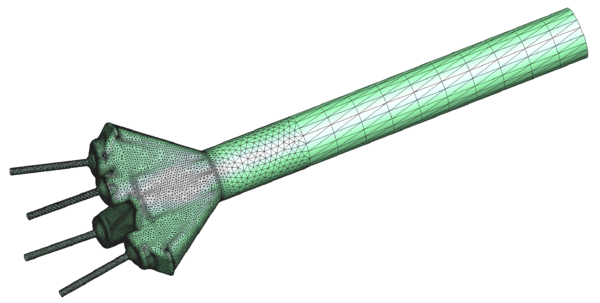
|
| Figure 55: Mesh used for the internal flow problem (8.14644x10⁵ tetrahedra). |
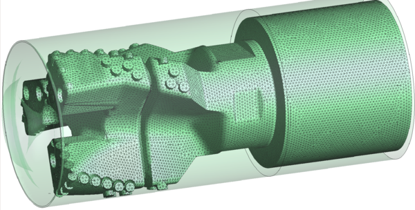
|
| Figure 57: Mesh used for the total flow problem (2.02281x10⁶ tetrahedra). |
Discretization of the fluid phase: Time step selection
The criterion for the time step selection responds to a balance between the need for an affordable computation and the accuracy required. In the context of turbulent flows, the CFL (Courant–Friedrichs–Lewy) number is used as a criterion to fix a higher limit to the time step in connection with the spatial resolution used. The CFL number is calculated as
|
|
(4.118) |
where is the magnitude of the velocity (relative to the mesh velocity). Explicit numerical schemes require that this condition is fulfilled to have numerical stability, but this case does not concern us, since our time scheme is theoretically unconditionally stable. Nonetheless, in order to have an accurate representation of the flow, it is recommended that anyway. In effect, when using a larger than one, it is impossible for the numerical scheme to resolve the dynamics of the smallest scales, which become filtered out.
The simulation of the PID system involves regions with very different characteristic velocities. Our criterion in choosing the time step has been to use values of the CFL smaller than one everywhere except inside the nozzles, where the CFL has been allowed to reach numbers in the range 2080. We thus expect to capture at most the larger-period instabilities inside the nozzles, while filtering out the fine details of the flow. This need not be a critical inaccuracy, since the particle are expected to respond sluggishly to these instabilities, see Section 4.7.4.
In the previous sections we have presented all the elements used to set up and perform the numerical simulations. In this section we describe the simulations that were finally performed and discuss the simulation results. We have considered two generic scenarios for the simulations: an internal flow scenario were we only look at the domain formed by the inner tubing from the inlet down to the tip of the nozzles; and an total flow scenario, where we simulate the whole domain. The internal flow simulations allow us to consider the flow with a greater level of detail at reasonable costs.
4.7.8 Simulations
In this subsections we present a selection of the simulation results. We start by listing the most relevant simulation settings.
Standard Settings
Parameters For the simulations we fix a number of parameters and options that we summarize in Table 14. These settings correspond to the standard case (SC) and any deviations from them will be explicitly remarked in their context.
| Parameter | Value | Description |
| Coupling Parameters | ||
| 1 | Include and (0 or 1) | |
| Contact parameters | ||
| 4.2x10⁻¹ | particle-wall friction coefficient | |
| 6x10⁻¹ | coefficient of normal restitution | |
| 1 | compute inter-particle contact (0 or 1) | |
| Numerical Parameters | ||
| internal | total | ||
| 2.6x10⁻³ m | 4x10⁻³ m | max. element size of irregular mesh 1 | |
| 1.1 | 2.7x101 | normalized width of elements adjacent to nozzle walls | |
| 1x10⁻⁴ s | 1x10⁻⁴ s | time step for the fluid-phase | |
| 5x10⁻⁷ s | 1.9x10⁻⁷ s | time step for the particles-phase |
Boundary conditions The boundary conditions imposed in all cases are a combination of strongly-imposed velocity conditions (uniform inlet velocity at the inlets and no-slip at the walls) and weakly imposed Neumann condition at the outlets (zero normal traction).
Internal flow results
We have run the standard internal flow simulations for a simulated time of 3x10⁻¹ s . This corresponds to more than five times the residence time of this part of the domain. Fig. 58 shows a plot of the evolution of the number of particles in time. Notice that, although the number increases at ever lower rates and one would expect it to not grow much above 1.3x10⁴, this is already almost twice the expected concentration for a uniform distribution of particles at their input rate, as obtained by multiplying by the volume of the domain.Figure 59 shows a snapshot of the particles phase with different vectorial results represented. Note the -fold ratio between the largest drag forces and the largest hydrodynamic force, due to the contribution of and around the entrance to the nozzles.
Figure 60 shows the velocity modulus contour maps on several cross-sections. The saturation value of the velocity is varied to highlight either the nozzles or the rest of the domain. Note the regularity of the flow in the inlet tube, where the Reynolds number is on the verge of turbulence. Note also the rotation-triggered vortices inside the three branches of the distribution chamber both in the horizontal and vertical directions.
Figure 61 shows two sets of streamlines at a particular time step. Fig. 61a shows a uniformly distributed selection of streamlines that passing through equally spaced points along the inlet tube cross-section. Fig. 61b shows a detail of streamlines passing through a segment of points inside a bisecting plane of one of the three branches of the distribution chamber. This figure highlights the convoluted direction of the flow in this recirculation zone.
Similarly, Fig. 62 shows a number of particles trajectories in the interval 0.250.3. Fig. 62b shows a detail where the particle temporary trapping in the recirculation zone is highlighted.
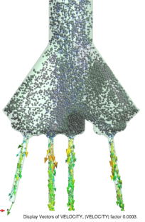
|
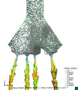
|
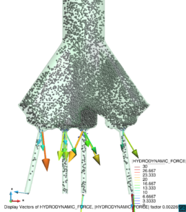
| |
| Figure 59: Particles flowing under the action of the flow at . The particles velocities, drag force and total hydrodynamic forces are shown. | |
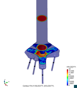
|
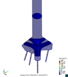
|
| transversal cuts | |
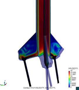
|
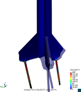
|
| vertical cuts | |
| Figure 60: Modulus of the velocity field at . | |
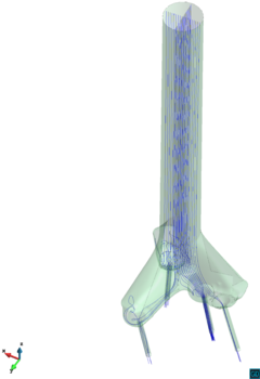
|
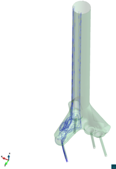
|
| (a) | (b) |
| Figure 61: Fluid streamlines at . Uniformly distributed streamlines (left) and detail of streamlines inside a vortical region (right). | |
Total flow results
The SC runs corresponding to the total flow have been run for a simulated time of 3.8x10⁻¹ s , the concentration time of the domain. In this case the mesh is slightly coarser than in the internal case for the inner tube and the focus is more on the annulus flow.
Figure 63 shows a sequence of three snapshots were the -component of the velocity is indicated with color on the particles surface. Note that significant inhomogeneities exist in the solid concentration, which indicates the need for further research to study this effect. Note however that the particle size has been exaggerated by a factor 2.5 to facilitate visualization.
Figure 64 shows a set of contour plots for a series of transversal and vertical cuts. As in Fig. 60, two sets of saturation velocities are used to highlight different regions of the flow; see also Fig. 65 for the corresponding streamlines. Note that the velocities in the internal flow are above the maximum of 8 m s-1 in large parts of the domain in Figs. (64a and 64d).
In Fig. 66 a sequence of contour plots of the level of wear on the rock bed is shown, demonstrating the potential for this approach to help in assessing the performance of changes in the design or the operation conditions. The action of the individual jets is clearly visible.
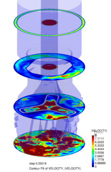
|
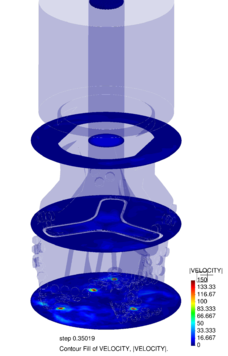
|
| transversal cuts | |
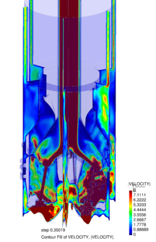
|
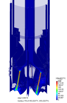
|
| vertical cuts | |
| Figure 64: Modulus of the velocity field at . | |
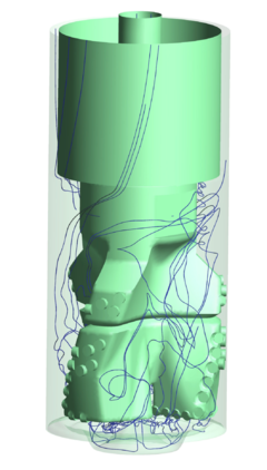
|
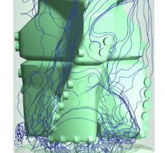
|
| (a) | (b) |
| Figure 65: Fluid streamlines at . Uniformly distributed streamlines (left) and detail of streamlines around the teeth (right). | |
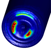
|
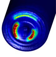
|
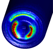
|
| Figure 66: Sequence of snapshots of the wear spread pattern evolution on the bed surface (red: intense wear; blue: light wear). | ||
Sensitivity Analyses
Given the uncertainty in the model parameters, it is interesting to investigate the influence of a few of them separately. This should help in concentrating the research efforts toward the most critical effects.
Coefficient of friction Let us investigate the effect of the most important parameters involved in the contact dynamics of the particles. Fig. 67 compares three snapshots corresponding to three different values of the coefficient of friction. The SC is shown in Fig. 67f, with a value of , given as representative of a typical of steel-on-steel contact by the consultancy firm. The other two figures show a snapshot of the same time step for and respectively, covering a wide range of values for what could be reasonably expected.
As seen in the figures, the effect of this parameter is very weak, and no clear trend can be observed. This can be explained in terms of the fact that the prevalent regime is on impact regime, where the particles are mostly bouncing off each other and off the surfaces, rather than rubbing against each other. It is known that the friction coefficient has a strong incidence on the angle of rebound in individual impacts [342]. However, this does not seem to bear any strong effect on the dynamics of the particles as a whole, probably due to the randomized character of the collective dynamics. Moreover, note that the accumulated number of particles is roughly equal in all cases; and idem with the wear pattern (see Fig. 68) indicating that the coefficient of friction plays little to no role in this problem.
Coefficient of normal restitution On the other hand, Fig. 69 shows the effect of variations in the coefficient of normal restitution on the dynamics of the particles. Again, snapshots taken at the same time steps are compared between simulations that only difference being the COR. The central figure corresponds to the SC, with , while Figs. 69b and 69f correspond to (highly dissipative) and (highly elastic). Clearly, the more dissipative case flows much more easily as the particles concentrate near the path of the dominating streamlines into the nozzles. When the COR is raised, the particles tend to occupy more space and accumulate more, as the number of particles in the domain goes from 8.759x10³ (close to the value of 7.85x10³ calculated by multiplying the input by the domain volume) for the most dissipative case, to 1.2469x10⁴ for the mildly dissipative case. This represents a 4.2x101 increase after only a quarter of a turn of the drill bit. Given the importance of the COR, therefore, and since (despite common practice) it is known that the COR is in fact not independent of the velocity [210], we must conclude that more work is needed to characterize the contact more accurately, especially given the large range of characteristic velocities for different regions of the domain.

|

|
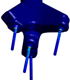
|
| (a) Rough contact () | (b) Standard case () | (c) Lubricated contact () |
| Figure 68: Effect of variations in the coefficient of friction on the wear pattern (red: intense wear; blue: light wear). | ||
Effect of neglecting inter-particle contacts Finally, we have investigated the importance of inter-particle contacts, since it would greatly simplify the analysis if we could do without them at all in the following ways:
- The computational cost would be greatly reduced, thanks to avoiding the most expensive parts of the DEM algorithm (force calculation and search)
- The parameter space would be reduced, since only the particle-wall contact parameters would matter
- It would be possible to alter (increase) the given concentration of particles to speed up the simulations, since each particle could be seen as an independent statistical test.
However, Fig. 71 shows that this simplification is not possible, at least at the current value of . When no interactions are used, the flow becomes more chaotic as the particles do not become entrained in the general flow towards the nozzles. Therefore, there is an increased rate of accumulation. Since the rate of inter-particle momentum transfer is null, slow particles trapped in the recirculation region tend to remain there for longer times, increasing the particles concentration artificially. Note also the conspicuous effect on the wear pattern in Fig. 72.

|

|
| (a) Standard case at t = 0.20s | (b) No interactions at t = 0.20s |
| Figure 72: Effect of inter-particle interactions on the wear pattern (red: intense wear; blue: light wear). | |
An attempt to simplify the problem: Pseudo-steady-state solution
In order to reduce the computational requirements of the analysis, we attempted to simplify the problem by averaging the fluid field over a short time interval, and take the averaged field as the fluid field for the computations with particles. The fluid-only simulation was run until a pseudo-steady state solution was reached. In this case, a temporal criterion was used, although a criterion based on the variation rate of the flow could have just as easily be used. When this point was reached, the flow was averaged over time, for an interval considered sufficient. Our criterion was to average at least for a period equivalent to half the residence time of the flow. Fig. 73 shows contour plots comparing the velocity field for a single snapshot for the SC case with the average field at the same instant. Note that the average field is only rotated with the drillbit, but does not change relative to that solid-body motion. Apparently, the main traits of the flow are well captured.
However, we found out that this strategy (on its own) completely fails when the particles are taken into account. The main reason for this seems to be that the strong fluid accelerations around the entrance to the nozzles, when averaged over time, creates zones of low pressure that act as particle traps. When the flow is dynamic, these low pressure pockets are unstable and the material acceleration changes vigorously in time, so that no trapping occurs. Instead, for the averaged field, these regions are capable of attracting particles and creating plugs (Fig. 74b). In Fig. 75a, the plug that forms is shown from a zoomed in view. Clearly the system does not work as expected.
A similar phenomenon is observed, even with no inter-particle interactions, see Fig. 74c. See also the zoomed in detail of the nozzle entrance in Fig. 75b where the pockets of overlapped particles take a toroidal shape.Measuring particle fluxes'
In this section we show results corresponding to an alternative geometry proposed by the consultancy company. Its design is shown in Fig. 76. Here the objective was to design a way to monitor any difference in the performance of each of the nozzles. We designed a variant of the usual DEM rigid walls of analytic type (see Section A.4). The surfaces keep the information about all the particles that cross them, their velocity and possibly other data, storing it all in a single HDF5 file for later analysis.
Figure 77 shows the resulting measurements for the nozzle surfaces shown in Fig. 76b. The method allows to monitor the performance of the nozzles, tracking both velocity and mass. Here we only show the number of particles per second that pass through each of the nozzles, identified by the labels shown in the insert of the same figure. The simulation was run for some time until the averages looked stable enough. Clearly, there are important differences in performance between the different nozzles. This type of result is a very good candidate for future validation, as the flux measurements can be obtained through experiments. Unfortunately, no data was available to us at the moment of writing this work, and such validation is left for the future.
(1) This number is approximated and is used by the mesh generator (advancing front) in [80] to build the mesh.
4.7.9 Discussion
Once more, we have applied our CFD-DEM numerical framework to perform simulations of a PID system using a one-way coupled strategy. We have demonstrated the possibilities of the technology by highlighting how a number of effects of relevance to the design of PID drillbits can be analysed for real geometries in operational conditions in a manageable amount of time.
We have demonstrated several interesting uses of such a technology in order to understand the PID systems better and aid in design, including
- The depiction of the internal flow of particles, including their distribution among the several pipes
- The prediction of wear concentrations, which can be used to improve the durability of designs
- The study of the outer flow patterns, which may help understand the movement of particles and possible sources of clogging and undesired accumulation.
- The study of the effect of changes in the number and granulometry of the metal particles
Our analysis suggests possible reductions in the parameter space, such as the elimination of the friction coefficient as an important parameter. It also highlights the importance of other parameters like the COR, which should be determined with sufficient precision in order to build a sufficiently accurate numerical tool. The same analysis also highlights the need for further research to determine the validity of our simplified coupling scheme, and in particular
- Extending the validity of the drag law by Shah for larger Reynolds numbers and testing it in instationary settings
- Studying the importance of lift
- Studying the need for more a sophisticated strategy that includes backward coupling, since the suspension is not lean enough to neglect the influence of the particles on the fluid phase a priori.
4.8 Backward-coupled particle-laden flows
As the solid fraction of particles in a given control volume raises, their influence on the flow becomes more important. This was already mentioned in Section 2.2.4 where, although the main concern was the motion of the particles, it was recognized that their mutual effects required an explanation via coupling to the fluid-phase, essentially through changes in its velocity. The issue was brought up again in Section 4.7, were it was recognized that neglecting these effects was probably causing important inaccuracies. In this section we tackle the issue, extending the formulation to include backward-coupling effect on the continuous phase.
For very lean flows, the study of the effects that the presence of particles have on the fluid is based on simple momentum transfer mechanisms. Specifically, the study of turbulence modulation by suspended particles [165] (see also [298] for a review on the most important variables involved) has been studied both from the theoretical [86,256] and numerical [126,360] points of view. The traditional approach has been to consider point sources to model the effect of the particles [322]. The success of such methods is mixed [113], although they certainly represent an improvement over the simple one-way coupled approach in some situations.
Nonetheless, the utility of point-source approaches are limited to very low solid fractions. For one, they do not take into account the volume-displacement effects due to the presence of a significant proportion of particles, even if only locally. The literature has provided some heuristic estimates for the need to take this volume displacement effects into account [116].
The theory of multicomponent media [109,179] provides an adequate framework to incorporate both effects into the analysis. This generalization of standard continuum media allows for the presence of an arbitrary number of continuum media superposed over the same spatial region, each with its own set of state variables and constitutive equations though allowing for coupling relations (differential or algebraic equations) to hold. The basic conservation equations are presented in Appendix H and can be taken as postulates to start the analysis [109]. It is however also possible to derive such equations by applying averaging techniques to the lower-scale description, just as the equations of the continuum can often be derived by applying averaging techniques to the microscopic description of the molecules.
We present in Appendix H a brief description of this averaging process that is a slight generalization of the volume averaging technique of Anderson and Jackson [8], see also [366]. This averaging process if of interest here as a tool to motivate the numerical method that is later described. We will focus on the fluid-phase averaged equations, since the particle-phase averaged equations are replaced by the DEM in the final algorithm.
4.8.1 CFD-DEM model
The hybrid CFD-DEM model is a multi-scale approach, where one simultaneously solves for the evolution of two coupled systems described at different levels of spatio-temporal detail. That is, the fluid is described at a coarser scale than the particles, and this scale is larger or equal to the mesh size used to discretize the continuous phase. The method has gained popularity in relatively recent times and its fundamentals can be found, for example in [372].
In order to construct the method, one takes a closed system of the two-fluid multicomponent equations that describe the evolution of the averaged variables, such as the velocity and volume fractions of the two phases involved. Then one replaces the balance equations (momentum and energy) relative to the particles by a DEM problem describing the evolution of the particles with appropriately modified coupling terms.
Our starting point are equations Eq.~H.54. We directly apply a common closure [355,182] to them, obtaining the following set of equations:
|
with
|
|
(4.124) |
and
|
|
(4.125) |
with for any and is the identity matrix and were we have abused the notation by denoting the averaged stress tensors with subindices instead of overhead indices, such as the ones used in Appendix H. Eq.~4.123 is an algebraic equation of the granular temperature, , where is the dissipation due to the inelastic nature of the inter-particle impacts, which depends solely on it. This equation is expected to be accurate enough at highly dense flows [355]. The pressure is taken as an independent variable and the fluid phase viscosity is taken as , the viscosity of the fluid itself.
The motivation behind Eq.~4.125 is that can be interpreted as the averaged force on the particles phase per unit volume applied by the surrounding fluid minus the term (see Eq.~13.54); where the latter term can in turn be interpreted as the averaged unperturbed flow force per unit volume of disperse phase. Thus, it is natural to model this term as the force terms in the equation of motion of a single particle (with the appropriate modifications due to the presence of neighbouring particles) over the volume of the particle, minus . Eq.~4.125 is one possibility, where the history and lift terms have been neglected. This is a very common practice for dense flows, where the drag force is typically dominant (most applications involve gas-solid flows) and the modelling uncertainties do not justified any more sophisticated models. The coefficient can be determined based on any variant Eq.~4.8.
It is not necessary to provide explicit closures for the particle-phase energy equation Eq.~4.123 since it, along with Eq.~4.122 are replaced by the DEM problem. The resulting coupled system of equations can be formally written as
|
where the superindices identify variables relative to particle and where the particle-averaged velocity and stress tensor do not explicitly appear in the system any more, allowing us to rename the fluid-averaged velocity and averaged stress tensor simply to and .
4.8.2 The continuous-phase problem for the backward-coupled fluid
Let be an open polyhedral domain of , where is the number of space dimensions, its boundary and the time interval of analysis. Let be a smooth real field on , where the overline denotes closure, representing the pointwise averaged fluid fraction. Using Eq.~4.125 into the first two equations in Eq.~4.126 yields the following system of equations:
|
where . In order to have a well-posed problem, it is necessary to provide an adequate set of boundary and initial conditions. Furthermore, the above system can be expressed as a convection-diffusion equation. Let us use both facts to define the problem we are interested in, i.e.find and such that
|
where
|
|
(4.137) |
and (summation is implied for repeated indices)
|
|
(4.138) |
where, for d = 3,
|
|
(4.139) |
|
|
(4.140) |
4.8.3 Finite Element Formulation
In this section we modify the formulation presented in Section 4.3.2 to suit the equations presented in Section 4.8.2.
Weak form
Let us come up with a suitable weak formulation of the problem defined by Eq.~4.133. First, the relevant function spaces are defined in a way completely analogous to what was done in Section 4.3.2. The weak form of the problem can be stated as find such that
|
|
(4.141) |
which is of the form Eq.~4.28 with
|
|
(4.142) |
and
|
|
(4.143) |
According to Eq.~4.50, the terms that must be added to the right hand side of the standard Galerkin formulation for the OSS formulation are the following
|
|
(4.144) |
Meanwhile the analogous terms for the ASGS method are obtained by replacing by in the integrals above.
On the other hand, let us now expand the term , which is present in both formulations. The formal adjoint of operator is obtained by transposing the matrices and changing the sign of odd-order terms; i.e.
|
|
(4.145) |
Consequently, for the case of negligible second derivatives (as in piecewise linear elements, where they exactly vanish within elements) we have:
|
|
(4.146) |
The resulting elemental matrices resulting from the FEM discretization of the formulations above are detailed in Appendix H for Q-ASGS and Q-OSS.
4.8.4 Backward coupling method
The backward coupling consists in the determination of the discrete counterparts of and from the DEM solution. According the theory developed in Appendix H, these variables are to be filtered from the disperse phase. Next we describe two alternative methods to do this.
Linear conservative projection
For every particle, its contribution to the discretized fluid fraction field affects its host element's nodes only. Let be the discrete form of the particles' phase volume fraction with nodal values . The linear conservative method is defined by
|
|
(4.147) |
where the same nomenclature as in Eq.~4.73 is used.
This scheme is conservative in the sense that the integrated total volume is conserved after projection. The linearity of the integral of the finite element discretization implies that the effect of many particles is the addition of the effect of each single particle. The conservation property can be readily checked by looking at the solid fraction field produced by a single particle. We should integrate the generated over the whole domain:
|
|
(4.148) |
where the last equality follows from the partition of unity property. Therefore, the global mass balance is conserved at all times. This conservation property also holds for other projected fields, such as the hydrodynamic forces exchanged with the particles, so that the total exchange forces between both phases fulfil an averaged version of Newton's Third Law.
The method just described is used to compute the averaged fields from a specific DEM solution, which can be assumed to be the latest value calculated. Moreover, it is also possible to smooth the solution in time by averaging the averaged fields over several DEM time steps, as is explicitly done with the technique that follows.
Polynomial filter
When a particle crosses over from one element to another, the fluid fraction field experiments a discontinuous jump proportional to the ratio of volumes of these two elements. To reduce this effect as well as to allow for a larger influence range of each particle, a filtering methodology has been devised in which each particle's volume is smeared over a number of nodes: those found inside a certain sphere concentric to the particle whose radius determines the extend of this smearing. This procedure starts by a search to determine, for each particle, which set of nodes falls inside the particle's influence domain. After that, each node within the domain is assigned a weight which monotonically decreases with distance to the particle, and so that their sum equals 1. This way, conservation is preserved as explained in Section 4.8.4. This procedure can be understood as a direct application of the filtering theory of Section H.1.4. In particular, within the point-particle approach particles are described as points, so that integrals over their volume must be replaced by Dirac deltas.
Let us assume we want to find the filtered value of an extensive quantity defined inside the particles' volume. Its filtered counterpart would be found by applying Eq.~13.59 to :
|
|
(4.149) |
where runs through all the particles in the domain and where is the integral of over the particle centred at . For the time filter we use a simple quadrature:
|
|
(4.150) |
where the indices indicate the time of evaluation. This operation can be performed accumulatively, at every DEM time step (or skipping a few at a time). However here we take
|
|
(4.151) |
So Eq.~4.150 becomes an evaluation at the current time. Thus, we can now concentrate on the space averaging by only assuming that the variables are evaluated at the current time step. Using this methodology, one immediately obtains a formula for the value of the filtered variables at the mesh nodes' locations and then extend their value over the whole domain using the FEM shape functions. For instance, the solid fraction can be calculated as (assuming all the variables are evaluated at the current time step)
|
|
(4.152) |
where is the volume of the -th particle and runs through the mesh nodes.
Note that it would be convenient to have the property
|
|
(4.153) |
Which is the analogous density-like property assumed to hold in the postulational approach of multicomponent continuum mechanics (see Appendix H). Using Eq.~4.152, such condition can be developed into
|
|
(4.154) |
where we define as a modified filter function. The condition above is verified, in particular if is a partition of unity . In our case, we have opted for a hybrid approach, where we use a generic bump function but impose the conservation property Eq.~4.153 a posteriori, by normalizing the contributions for each . In this way, we guarantee that information is smoothed, that particles closer by are weighed more highly and that Eq.~4.153 holds. We have found this scheme to be quite robust, avoiding the instabilities that might appear when the size of the particles becomes closer to the elemental size when using more standard approaches [276].
4.8.5 Final algorithm
The algorithm used for the two-way coupled model is very similar to the one described in Section 4.7.6, but obviously with the modified finite element formulation of the coupled problem that we discussed in the present section. Algorithm 7 shows the basic layout of this algorithm where the main difference with respect to Algorithm 5 is the addition of a backward-coupling step, designated in the pseudo-code with the name . The background coupling does not need to be done at every sub-time step. In fact once every fluid time step is normally enough 1 if no time filtering is applied. The variable has been introduced to express this new substepping for the background coupling.
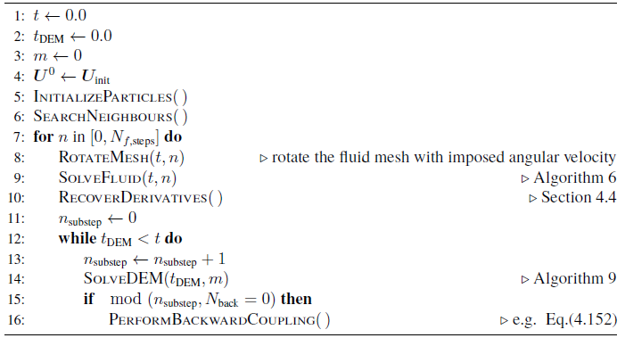
|
|
Algorithm. 7 Two-way-coupled two-phase algorithm. |
(1) It is not logically necessarily so, since it is possible that depends on . This means that it is conceivable to have the solid fraction calculated more often than the fluid, when its value needs to be repeatedly updated within one fluid time step during the integration of the particles motion.
4.9 Application example: fluidized bed
In this section we apply the theory presented above to a representative problem in which the backward coupling is unavoidable. This problem was studied numerically recently by Boyce et al. [42] where the limitations of the volume averaging approach in the CFD-DEM were discussed and highlighted. Our objective here is to see if our finite element-based approach can obtain the same qualitative behaviour obtained with a more conventional approach and to check whether the same problems observed there are reproduced here.
The problem at hand is the simulation of a gas-fluidized bed of Geldart-D type [143] particles (poppy seeds), that where experimentally studied previously by Holland et al. [170]. The container is cylindrical, with a circular base. The geometry corresponds to configurations 2 and 3 in Boyce et al. [42], and it is depicted in Fig. 78a. The initial bed size is of 5x101 . The most important input parameters are detailed in Table 15. In the original work hexahedral cells arranged in a structured way were used for the fluid discretization. We instead employed the sequence of irregular tetrahedral meshes shown in Fig. 78, were the average sizes (expressed as fractions of the particles' diameter) are calculated as the side of a regular tetrahedron that has the same volume as the average volume of the tetrahedra in the mesh. The average sizes are comparable to the ones used considered in Boyce et al. [42].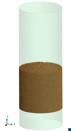
|
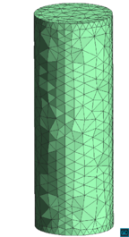
|
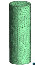
|
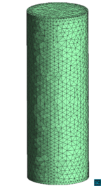
|
| geometry | |||
| Figure 78: Model geometry with initial particles bed and computational meshes considered. | |||
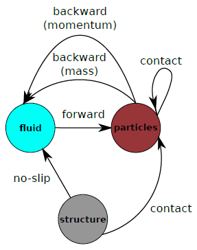
|
| Figure 81: Diagram of phase interactions accounted for in the fluidized bed simulation. |
| Parameter | Value | Description |
| Fluid parameters | ||
| 1 kg m-1 ^3 | density of fluid | |
| 1.5x10⁻⁵ s m-1 ^2 | kinematic viscosity | |
| Particles parameters | ||
| 1.2x10⁻³ m | particles' diameter | |
| 1x10⁻¹ | friction coefficient 1 | |
| 9x10² kg m-1 ^3 | apparent density of particles | |
| COR | 2x10⁻¹ | coefficient of normal restitution |
Figure 78b shows a window of the pressure in time as measured at a single point, for the different meshes considered. The pressure values are made dimensionless by dividing them by the average pressure drop in the first 5x101 from the bottom of the bed, as measured on the symmetry axis of the container. From the graph, it is clear that while the average pressure is not sensitive to the mesh size, but the amplitude of its oscillations does show this dependency. Moreover, Fig. 78b shows the dependency of the oscillation frequency with respect to the mesh size. These frequencies were obtained by identifying peaks in the note that this dependency is clear although somewhat less marked than that observed in Boyce et al. [42], where a method analogous to the standard method was used for the coupling. We can conclude therefore that our method suffers from the same mesh-dependent problems reported by others. This may be due to intrinsic limitations of the filtered equations themselves and not the coupling method, although more work is needed to determine this.
(1) No difference is made between the particle-wall and the particle-particle friction coefficients in either [355] nor [170]. We have therefore assumed they coincide.
4.10 Summary
In this chapter we have described a numerical approach that can be used to simulate a wide range of particle-laden flows. The scope of this chapter has greatly widened with respect to the preceding two, considering a much greater range of physical situations, including larger particle Reynolds numbers, non-Newtonian fluids and dense suspensions, but also in the number of elements being simulated, including the fluid and the consideration of inter-particle contacts. In general, the core of the discourse has furthermore revolved around a varied set of applications, associated with the industry and the development of a versatile application capable of dealing with a large range of situations.
Nonetheless, we have made some genuine contributions of academic interest:
- A review of the state of the art in derivative recovery including methods associated with the FEM with a practical discussion of their implementation for their use in particle-laden flow simulations. We concluded with the recommendation of using the PPR method with a fall-back to the standard recovery method for difficult areas. When the memory resources are scarce, the standard recovery methodology is robust and reasonably accurate for first-order derivatives.
- The application of the VMS methodology to develop a stabilized FEM formulation for the CFD-DEM
- A backward-coupling methodology based on the notion of filtering the disperse phase that unties the discretization from the filtering scales and largely avoids the limitations associated with the element size to particle diameter ratio.
We have looked at three applications of the described methodology with industrial interest, each one illustrating a different coupling scheme. The first one deals with the phenomenon of bubble-trapping in T-junction bifurcations in liquid piping systems. We showed that the methodology captures the qualitative trends when compared to the literature, although some quantitative discrepancies remain. We have pointed to a possible explanation based on a small difference in the formulation, although it could be due to small differences in the fluid solution. The matter therefore requires further research in order to move toward robust quantitative predictability in such systems.
The second example explores a drilling system for the oil and gas industry. We used a one-way coupled approach to produce simulations of the flow of steel particles within the system. We gave a sensitivity analysis and made conjectures about the parameters that may be of lesser importance. We showed how the tool can be used by engineers to estimate the flux of particles within the system with the use of flux-measuring surfaces and how the system can be used to identify the areas more vulnerable to wear. Unfortunately, no experimental data was made available to us, although we are working toward undertaking this task in the future.
The third example showed a fluidized bed, as a paradigmatic case for the application of the two-way coupled methodology that we have developed, but that can be used in many other settings, including that of the second example, which is currently under study. This example showed how the system correctly predicted the formation of bubbles, although we reproduced the difficulties encountered by Boyce et al. [42] regarding the estimation of the bubbling frequency. Again, it is our intention to keep studying this problem taking the developments presented here as a foundation.
In summary, we have presented a remarkably general tool that is able to greatly extend the range of application considered in the preceding two chapters. The tool is of interest to many industrial problems and its potential has been demonstrated in a set of tests representative of different coupling schemes.
5 Conclusions and Future work
The particular technical advances and findings have already been summarized at the end of each chapter. Consequently, we dedicate the next lines to making only a number of general remarks about the work achieved in relation to the initial goals and some speculations about the future relevance of our contributions. We close our work discussing a selection of the topics that we have left for future work.
5.1 Concluding remarks
It is time to look back to the objectives that we set in Section 1.2 to see how far we went about fulfilling them. Let us go over the list once again:
- To develop an algorithm that combines the discrete element method and the finite element method to simulate particle-laden flows with the following list of requisites:
- capability of dealing with a wide range of regimes, including the possibility to have regions with dense and dispersed suspensions simultaneously: We demonstrated the capabilities of our coupled code in Chapter 4. The backward-coupled formulation is general enough to allow for dense flows and default to the one-way coupled formulation in the limit of small solid volume fractions.
- use of the finite element method to discretize the fluid: Done.
- use of the discrete element method to model the particles: Done.
- To study the range of applicability of the Maxey–Riley equation as a model for the motion of the individual particles submerged in a fluid, improving the current knowledge on the subject and generating, where possible, practical estimates of direct application to numerical modelling: Chapter 2 was fully dedicated to this task in what, we believe is the most comprehensive analysis of the range of applicability of the MRE to date. Naturally, our analysis is still far from exhaustive, having left some of the most important effects for future work, such as the first effects of the proximity of walls and a more complete study of the presence of lift and also complicated matters such as the effect of a systematic orientation in non-symmetrical particles. Furthermore, the conclusions of our analysis need to be thoroughly tested by experimental and numerical means. Such effort would help to both strengthen the reliability of the estimates and perhaps also discover weaknesses in some of the simplifying assumptions used.
- To study current alternatives for the numerical treatment of the history term in the equation of motion and compare them: We reviewed in Chapter 3 some of the most recent techniques and compared them, updating the state of the art with respect to these novelties. We also made a long-needed connection between the literature on fractional differential equations and the MRE, which has not been sufficiently exploited.
- To improve on the method of quadrature (the history term involves a time integral, as will be explained later) proposed by van Hinsberg et al. [353] and provide a detailed study of its efficiency and accuracy, providing convincing evidence that it is not necessary to neglect this term to have an efficient numerical method: This is the central subject of Chapter 3, where we considered a generalized version of the problem originally posed by van Hinsberg et al. We also provided a detailed study of the efficiency of the method, concluding that it opens the door to a systematic inclusion of the history force in disperse particle-laden flows due to its reasonable cost.
- To report an account of relevant application examples of the proposed strategy with interest to the industry, as well as of the different technologies developed for their particular requirements: In Chapter 4 we have reported three examples representative of different coupling regimes relevant to different industries, including very dispersed, internal flows relevant to microfluidics (Section 4.6); the higher density, although still not too high of relevance to the PID system for the oil and gas industries (Section 4.7) and fully coupled, high density flows, especially relevant to problems where regions with very high density of particles are likely to develop, such as fluidized beds or bed formation in pipes (Section 4.9).
- To generalize a stabilized finite element method and use it to discretize the backward-coupled flow equations: We gave such formulation in Chapter 4, although we left the numerical analysis for future work.
- To develop a suitable inter-phase coupling strategy: We provided two formulations in Section 4.8.4. The filter-based method provided there is robust with respect to local peaks in the solid density, as it smears the variables over several elements, avoiding the appearance of instabilities due to too strong oscillations in the local momentum exchange. However, we have reproduced some of the problems found in the literature regarding the mesh-dependence of the solutions (see Section 4.9) that do require further work.
In general terms, we believe we have been able to fulfil, at least partially, all of the goals we set at the beginning of this work. Looking back, we find that the initial focus, which had been intended to fall upon the development of a two-way coupled algorithm (with a detailed numerical analysis to go with it) shifted toward a study of the single-particle coupling terms. The reason is the unexpected discovery of the large complexity and richness of this area and the need to understand it deeply in order to move toward a macroscopic formulation that, in the end, must be based on it.
The work in Chapter 2 is a reflection of this study. It is our intention to summarize the most valuable results from Chapter 2 in a paper, currently in production.
We also hope that its output is useful as a starting point for a gradual, organic evolution of the range of applicability of the MRE. We are convinced that this type of knowledge will in the future be much more tightly associated with the model equation itself thanks to the latest advances in data processing and the internet. We envision that not only the limits of applicability will be associated to the model, but also the information about the certainty of these limits, contradictory data, the sources of each piece of information, associated and related models and experimental data etc.
Generalizing, we see no impediment for this scenario to also arise with many other equations, perhaps in very different fields. For that, it is important to proceed more systematically and get over the current times, where such information is held, in a unified manner, only in the brains of experts.
As a side effect of this careful study, we came across the world of the very disperse suspensions at very low particle Reynolds numbers, which require special care in formulating very precise algorithms. With the idea of building a general tool, we were faced with the necessity to include the history term of the MRE, which resulted in 3. The work contained in this chapter has been published in [63].
The tests run in Chapter 3 helped creating a generalistic CFD-DEM code with a solid foundation, that we hope will be very much enlarged in its capabilities in the near future. These tests are used as benchmarks to keep the code constantly verified.
Finally, some of the work in Chapter 4 has started interesting lines of research, such as the derivative recovery algorithms, which we plan to make generally available to the users of Kratos, since they can be of interest for many uses, including post-processing and error estimation. Similarly, many hydrodynamic interaction laws have been made available and have already found application in several areas apart from the ones demonstrated here, including pneumatic conveying of seeds and even some applications in the study of expansive clays at colloidal scale.
5.2 Future work
Our work has covered a rather wide range of topics which means that many more doors have been opened than closed. Our study in Chapter 2 was exhaustive by aspiration but many topics were only touched on superficially. The study of the history force from Chapter 3 served as an introduction on several techniques related to the numerical treatment of fractional differential equations that where simply mentioned and even our proposed method was left with several questions to be answered. But it is probably Chapter 4 that introduced the most topics that had to be left for the future.
5.2.1 Range of applicability of the MRE and scaling analysis
The limits collected in Section 2.4 should be tested to give empirical evidence to each of the numbers summarized in the tables we have provided. We are currently planning a campaign to document existing results and identify the weakest estimates. Numerical experiments should be useful in this respect, perhaps using isotropic turbulence with a DNS technique.
The estimates in Section 2.2.4 contain particular uncertainty, due to the complexity of the formulation and the many simplifications. A very interesting experiment which we believe has not been performed yet is a systematic study of the effect of neighbours as
- Short-range effects, by comparing the motion of particles in a numerically simulated turbulent flow with and without these effects. To simulate these short-range effects one could use simplified formulations such as the one by [292].
- Long-range effects, by comparing disperse flows with and without two-way coupling, taking into account what part of the interaction is treated indirectly, though the interaction with the fluid; and what part is treated directly. To this respect the work of Huck et al. [173] is relevant.
5.2.2 More on the history force calculation
In Section 3.5.1 we briefly visited the possibility of using extrapolation techniques to enhance the Grünwald–Letnikov formulation of the fractional derivative to produce high-order quadrature techniques to calculate the history term in the MRE. However, we never implemented such techniques to calculate the motion of submerged particles, since this required unspecified changes in the quadrature algorithms that require considerable work. Nonetheless, we think this path can lead to elegant methods to obtain high-order quadrature schemes and therefore the matter deserves further study.
5.2.3 Derivative recovery
The unsuccessful stabilization of the formulation of Pouliot et al. [282] for some regular meshes spoilt a method that otherwise provided a set of very positive properties, including:
- Very high accuracy when it works
- Good properties at the boundary [282]
- A structure naturally apt for an implementation within a typical FEM framework, facilitating parallelization (as the method would inherit all the parallelization work already done in the framework)
We still believe it might be possible to fix the method in a robust way, but the matter is not trivial and we had to leave it for future work.
5.2.4 Future developments for backward coupling
The inaccuracies that we reported in Section 4.9 with respect to the bubbling frequency are a matter of concern. In line with [42], we suspect a modification of the coupling scheme might help. It is equally important to study the mesh-dependence of the method and how it can be dealt with effectively. All these matters require further work.
5.2.5 Future developments for the applications
The various application examples that we have presented in Chapter 4 have also lead to various interesting paths for future work. For instance, ongoing work on the PID systems is requiring further considerations with regards to some of the assumptions taken so far. Here is a selection of the most important if these:
Non-Newtonian drag laws
The hydrodynamic interactions assumed to be valid for the steel particles in power-law type drilling mud are based on a combination of effects including the drag formulation of Shah et al. [312]. This formulation was however only validated for free-falling particles at their terminal velocity and only up to particle Reynolds numbers slightly lower than the most extreme values observed in our simulations. But for quantitatively accurate simulations, it is essential to keep validating the whole hydrodynamic model in general and the drag law in particular. Specifically, it is important to extend the range of applicability of the formulation beyond the current Reynolds numbers and verify its accuracy in instationary flows.
Lift
The importance of lift (hydrodynamic forces perpendicular to the slip velocity) has not been studied in the examples reported in this work. There is currently, to our knowledge, no available formulation for non-Newtonian fluids that can be used beyond very small Reynolds numbers [175]; although some authors have simply used formulations for Newtonian fluids using the local effective viscosity [264,2]. This matter deserves further research, either to develop a formulation or to provide an estimation of the circumstances where these effects can be neglected or just approximated using the Newtonian formulation.
Backward coupling
Our simulations showed the need to explore the importance of the backward coupling in the PID simulations. Our code should be extended to the non-Newtonian case and a sensitivity study performed to explore this issue.
5.2.6 Backward Coupled CFD-DEM flows
We have barely touched upon the development of FEM-based methods to solve the CFD-DEM fluid-phase equations. Our implementation showed good behaviour and stability in the examples run, but no mathematical proof was provided to back it up. The matter is nontrivial and trying analogous techniques to the ones reported in Codina [77] would not work here, since the resulting stabilised bilinear form Eq.~4.142 is not in fact coercive, property on which is based the stability proof in that work. Our preliminary tests with manufactured solutions (not reported here) did indeed show the right optimally-convergent behaviour, at least in the stationary case, with an arbitrarily-set solid fraction field. In any case, more work is needed in this area to arrive at solid conclusions on the stability and accuracy properties of the numerical method.
5.2.7 Backward-coupling scheme
Our filtering-based approach has yielded good behaviour that is less prone to instabilities caused by the presence of too-large particles (as compared to the fluid elements) in our experience. However, no systematic work has been done on this matter so far. The examples presented in Section 4.9 showed there are still deficiencies in the overall approach and the coupling scheme is one of the most promising suspects to be responsible for the error. Also, some mesh-dependence was observed and the method should in principle become mesh-independent for large enough filtering radii. The issue of fixing the filtering radii as well as choosing the filtering kernel should therefore be analysed in relation to the problem of mesh-dependence. This question surely provides fecund material for future work.
References
[1] Agarwal, R. P., Benchohra, M., and Hamani, S. (2010). A survey on existence results for boundary value problems of nonlinear fractional differential equations and inclusions. Acta Applicandae Mathematicae, 109(3):973–1033.
[2] Akhshik, S., Behzad, M., and Rajabi, M. (2015a). CFD–DEM approach to investigate the effect of drill pipe rotation on cuttings transport behavior. Journal of Petroleum Science and Engineering, 127:229–244.
[3] Akhshik, S., Behzad, M., and Rajabi, M. (2015b). CFD–DEM Model for Simulation of Non-spherical Particles in Hole Cleaning Process. Particulate Science and Technology, 33(5):472–481.
[4] Aliseda, A., Cartellier, A., Hainaux, F., and Lasheras, J. C. (2002). Effect of preferential concentration on the settling velocity of heavy particles in homogeneous isotropic turbulence. Journal of Fluid Mechanics, 468(October):77–105.
[5] Aliseda, A. and Lasheras, J. C. (2011). Preferential concentration and rise velocity reduction of bubbles immersed in a homogeneous and isotropic turbulent flow. Physics of Fluids, 23(9):093301.
[6] Anderson, J. D. (2005). Ludwig Prandtl's Boundary Layer. Physics Today, 58(12):42–48.
[7] Anderson, J. D. J. (1997). A History of Aerodynamics. Cambridge University Press, Cambridge.
[8] Anderson, T. B. and Jackson, R. (1967). Fluid Mechanical Description of Fluidized Beds. Equations of Motion. Industrial & Engineering Chemistry Fundamentals, 6(4):527–539.
[9] ANSYS (2016). ANSYS Fluent Theory Guide–Release 17.0.
[10] Antypov, D. and Elliott, J. A. (2011). On an analytical solution for the damped Hertzian spring. EPL (Europhysics Letters), 94(5):50004.
[11] Apte, S., Mahesh, K., Moin, P., and Oefelein, J. (2003). Large-eddy simulation of swirling particle-laden flows in a coaxial-jet combustor. International Journal of Multiphase Flow, 29(8):1311–1331.
[12] Armenio, V. and Fiorotto, V. (2001). The importance of the forces acting on particles in turbulent flows. Physics of Fluids, 13(8):2437–2440.
[13] Auton, T. R. (1987). The lift force on a spherical body in a rotational flow. Journal of Fluid Mechanics, 183(-1):199.
[14] Auton, T. R., Hunt, J. C. R., and Prud'Homme, M. (1988). The force exerted on a body in inviscid unsteady non-uniform rotational flow. Journal of Fluid Mechanics, 197(-1):241.
[15] Ayala, O., Grabowski, W. W., and Wang, L. P. (2007). A hybrid approach for simulating turbulent collisions of hydrodynamically-interacting particles. Journal of Computational Physics, 225(1):51–73.
[16] Azaiez, J. (2008). Bubbles, drops and particles in non-newtonian fluids. R. P. Chhabra. The Canadian Journal of Chemical Engineering, 85(2):251–252.
[17] Babuska, I. and Miller, A. (1984). The post-processing approach in the finite element method—part 1: Calculation of displacements, stresses and other higher derivatives of the displacements. International Journal for Numerical Methods in Engineering, 20(6):1085–1109.
[18] Baffet, D. and Hesthaven, J. S. (2017). A Kernel Compression Scheme for Fractional Differential Equations. SIAM Journal on Numerical Analysis, 55(2):496–520.
[19] Balachandar, S. (2009). A scaling analysis for point–particle approaches to turbulent multiphase flows. International Journal of Multiphase Flow, 35(9):801–810.
[20] Balachandar, S. and Maxey, M. (1989). Methods for evaluating fluid velocities in spectral simulations of turbulence. Journal of Computational Physics, 83(1):96–125.
[21] Barber, R. W. and Emerson, D. R. (2006). Challenges in Modeling Gas-Phase Flow in Microchannels: From Slip to Transition. Heat Transfer Engineering, 27(4):3–12.
[22] Barker, T., Schaeffer, D. G., Bohorquez, P., and Gray, J. M. N. T. (2015). Well-posed and ill-posed behaviour of the -rheology for granular flow. Journal of Fluid Mechanics, 779:794–818.
[23] Batchelor, G. K. (1972). Sedimentation in a dilute dispersion of spheres. Journal of Fluid Mechanics, 52(02):245.
[24] Batchelor, G. K. (1982). Sedimentation in a dilute polydisperse system of interacting spheres. Part 1. General theory. Journal of Fluid Mechanics, 119(-1):379.
[25] Bec, J. (2003). Fractal clustering of inertial particles in random flows. Physics of Fluids, 15(11):L81–L84.
[26] Bec, J., Biferale, L., Cencini, M., Lanotte, A., Musacchio, S., and Toschi, F. (2007). Heavy Particle Concentration in Turbulence at Dissipative and Inertial Scales. Physical Review Letters, 98(8):084502.
[27] Bec, J., Biferale, L., Cencini, M., Lanotte, A. S., and Toschi, F. (2006). Effects of vortex filaments on the velocity of tracers and heavy particles in turbulence. Physics of Fluids, 18(8):081702.
[28] Bec, J., Biferale, L., Cencini, M., Lanotte, A. S., and Toschi, F. (2011). Spatial and velocity statistics of inertial particles in turbulent flows. Journal of Physics: Conference Series, 333:012003.
[29] Bec, J., Biferale, L., Lanotte, A. S., Scagliarini, A., and Toschi, F. (2010). Turbulent pair dispersion of inertial particles. Journal of Fluid Mechanics, 645:497.
[30] Bec, J., Celani, A., Cencini, M., and Musacchio, S. (2005). Clustering and collisions of heavy particles in random smooth flows. Physics of Fluids, 17(7):073301.
[31] Beetstra, R., van der Hoef, M. A., and Kuipers, J. A. M. (2007). Drag force of intermediate Reynolds number flow past mono- and bidisperse arrays of spheres. AIChE Journal, 53(2):489–501.
[32] Belhamadia, Y., Fortin, A., and Chamberland, É. (2004). Anisotropic mesh adaptation for the solution of the Stefan problem. Journal of Computational Physics, 194(1):233–255.
[33] Bellani, G. and Variano, E. A. (2012). Slip velocity of large neutrally buoyant particles in turbulent flows. New Journal of Physics, 14(12):125009.
[34] Ben Salem, M. and Oesterle, B. (1998). A shear flow around a spinning sphere: numerical study at moderate reynolds numbers. International Journal of Multiphase Flow, 24(4):563–585.
[35] Benes, K., Tong, P., and Ackerson, B. J. (2007). Sedimentation, Péclet number, and hydrodynamic screening. Physical Review E, 76(5):056302.
[36] Benson, D. A., Meerschaert, M. M., and Revielle, J. (2013). Fractional calculus in hydrologic modeling: A numerical perspective. Advances in Water Resources, 51:479–497.
[37] Berg-Srensen, K. and Flyvbjerg, H. (2005). The colour of thermal noise in classical Brownian motion: a feasibility study of direct experimental observation. New Journal of Physics, 7:38–38.
[38] Betchen, L. J. and Straatman, A. G. (2009). An accurate gradient and Hessian reconstruction method for cell-centered finite volume discretizations on general unstructured grids. International Journal for Numerical Methods in Fluids, 62(9):n/a–n/a.
[39] Bian, X., Kim, C., and Karniadakis, G. E. (2016). 111 years of Brownian motion. Soft Matter, 12(30):6331–6346.
[40] Bombardelli, F. a., González, A. E., and Niño, Y. I. (2008). Computation of the Particle Basset Force with a Fractional-Derivative Approach. Journal of Hydraulic Engineering, 134(10):1513–1520.
[41] Bosse, T., Kleiser, L., and Meiburg, E. (2006). Small particles in homogeneous turbulence: Settling velocity enhancement by two-way coupling. Physics of Fluids, 18(2):027102.
[42] Boyce, C. M., Holland, D. J., Scott, S. A., and Dennis, J. S. (2015). Limitations on Fluid Grid Sizing for Using Volume-Averaged Fluid Equations in Discrete Element Models of Fluidized Beds. Industrial & Engineering Chemistry Research, 54(43):10684–10697.
[43] Brady, J. (1988). Stokesian Dynamics. Annual Review of Fluid Mechanics, 20(1):111–157.
[44] Bragg, A. D. and Collins, L. R. (2014). New insights from comparing statistical theories for inertial particles in turbulence: I. Spatial distribution of particles. New Journal of Physics, 16(5):055013.
[45] Bragg, A. D., Ireland, P. J., and Collins, L. R. (2015). On the relationship between the non-local clustering mechanism and preferential concentration. Journal of Fluid Mechanics, 780:327–343.
[46] Brandts, J. and Michal, K. (2000). History and future of superconvergence in three-dimensional finite element methods. Utrecht University Repository (preprint), pages 1–10.
[47] Brennen, C. E. (2005). Fundamentals of Multiphase Flow, volume 9780521848. Cambridge University Press, Cambridge.
[48] Brenner, H. (1996). The Stokes hydrodynamic resistance nonspherical particles. Chemical Engineering Communications, 148-150(1):487–562.
[49] Brinkman, H. C. (1949). A calculation of the viscous force exerted by a flowing fluid on a dense swarm of particles. Flow, Turbulence and Combustion, 1(1):27.
[50] Brown, P. P. and Lawler, D. F. (2003). Sphere Drag and Settling Velocity Revisited. Journal of Environmental Engineering, 129(3):222–231.
[51] Brzeziski, D. W. and Ostalczyk, P. (2016). About accuracy increase of fractional order derivative and integral computations by applying the Grünwald–Letnikov formula. Communications in Nonlinear Science and Numerical Simulation, 40:151–162.
[52] Burg, C. and Erwin, T. (2009). Application of Richardson extrapolation to the numerical solution of partial differential equations. Numerical Methods for Partial Differential Equations, 25(4):810–832.
[53] Calzavarini, E., Volk, R., Bourgoin, M., Léveque, E., Pinton, J., and Toschi, F. (2009). Acceleration statistics of finite-sized particles in turbulent flow: the role of Faxén forces. Journal of Fluid Mechanics, 630(10):179.
[54] Calzavarini, E., Volk, R., Léveque, E., Pinton, J.-F., and Toschi, F. (2012). Impact of trailing wake drag on the statistical properties and dynamics of finite-sized particle in turbulence. Physica D: Nonlinear Phenomena, 241(3):237–244.
[55] Candelier, F. (2008). Time-dependent force acting on a particle moving arbitrarily in a rotating flow, at small Reynolds and Taylor numbers. Journal of Fluid Mechanics, 608:319–336.
[56] Candelier, F. and Angilella, J. R. (2006). Analytical investigation of the combined effect of fluid inertia and unsteadiness on low-Re particle centrifugation. Physical Review E, 73(4):047301.
[57] Candelier, F., Angilella, J. R., and Souhar, M. (2004). On the effect of the Boussinesq–Basset force on the radial migration of a Stokes particle in a vortex. Physics of Fluids, 16(5):1765–1776.
[58] Candelier, F., Einarsson, J., Lundell, F., Mehlig, B., and Angilella, J.-R. (2015a). Erratum: Role of inertia for the rotation of a nearly spherical particle in a general linear flow. Physical Review E, 92(5):059901.
[59] Candelier, F., Einarsson, J., Lundell, F., Mehlig, B., and Angilella, J.-R. (2015b). Role of inertia for the rotation of a nearly spherical particle in a general linear flow. Physical Review E, 91(5):053023.
[60] Candelier, F. and Souhar, M. (2007). Time-dependent lift force acting on a particle moving arbitrarily in a pure shear flow, at small Reynolds number. Physical Review E, 76(6):067301.
[61] Cao, J. and Xu, C. (2013). A high order schema for the numerical solution of the fractional ordinary differential equations. Journal of Computational Physics, 238:154–168.
[62] Capecelatro, J. and Desjardins, O. (2013). An Euler–Lagrange strategy for simulating particle-laden flows. Journal of Computational Physics, 238:1–31.
[63] Casas, G., Ferrer, A., and Oñate, E. (2018). Approximating the Basset force by optimizing the method of van Hinsberg et al. Journal of Computational Physics, 352:142–171.
[64] Casas, G., Mukherjee, D., Celigueta, M. A., Zohdi, T. I., and Onate, E. (2017). A modular, partitioned, discrete element framework for industrial grain distribution systems with rotating machinery. Computational Particle Mechanics, 4(2):181–198.
[65] Celigueta, M., Casas, G., Latorre, S., and Arrufat, F. (2018). DEMPack.
[66] Celigueta, M. A., Deshpande, K. M., Latorre, S., and Oñate, E. (2016a). A FEM-DEM technique for studying the motion of particles in non-Newtonian fluids. Application to the transport of drill cuttings in wellbores. Computational Particle Mechanics, 3(2):263–276.
[67] Celigueta, M. A., Deshpande, K. M., Latorre, S., and Oñate, E. (2016b). A FEM-DEM technique for studying the motion of particles in non-Newtonian fluids. Application to the transport of drill cuttings in wellbores. Computational Particle Mechanics, 3(2):263–276.
[68] Chen, H. and Li, J. (2016). Bubble Collisions in Microchannels Affected by Hydrodynamic Pressures. Tribology Online, 11(2):281–287.
[69] Chen, M. and Deng, W. (2014). Fourth Order Accurate Scheme for the Space Fractional Diffusion Equations. SIAM Journal on Numerical Analysis, 52(3):1418–1438.
[70] Chen, S., Bartello, P., Yau, M. K., Vaillancourt, P. A., and Zwijsen, K. (2016). Cloud Droplet Collisions in Turbulent Environment: Collision Statistics and Parameterization. Journal of the Atmospheric Sciences, 73(2):621–636.
[71] Choi, J.-I., Park, Y., Kwon, O., and Lee, C. (2016). Interparticle collision mechanism in turbulence. Physical Review E, 93(1):013112.
[72] Chong, K., Kelly, S. D., Smith, S., and Eldredge, J. D. (2013). Inertial particle trapping in viscous streaming. Physics of Fluids, 25(3):033602.
[73] Chun, J., Koch, D. L., Rani, S. L., Ahluwalia, A., and Collins, L. R. (2005). Clustering of aerosol particles in isotropic turbulence. Journal of Fluid Mechanics, 536(May):219–251.
[74] Citro, V., Siconolfi, L., Fabre, D., Giannetti, F., and Luchini, P. (2017). Stability and Sensitivity Analysis of the Secondary Instability in the Sphere Wake. AIAA Journal, 55(11):3661–3668.
[75] Clercx, H. J. H. and Schram, P. P. J. M. (1992). Brownian particles in shear flow and harmonic potentials: A study of long-time tails. Physical Review A, 46(4):1942–1950.
[76] Cockburn, B. and Mustapha, K. (2015). A hybridizable discontinuous Galerkin method for fractional diffusion problems. Numerische Mathematik, 130(2):293–314.
[77] Codina, R. (2001). A stabilized finite element method for generalized stationary incompressible flows. Computer Methods in Applied Mechanics and Engineering, 190(20-21):2681–2706.
[78] Codina, R. (2002). Stabilized finite element approximation of transient incompressible flows using orthogonal subscales. Computer Methods in Applied Mechanics and Engineering, 191(39-40):4295–4321.
[79] Coimbra, C. F. M. and Rangel, R. H. (2001). Spherical particle motion in harmonic stokes flows. AIAA Journal, 39(9):2001–1673.
[80] Coll, A. and Ribó, R. and Pasenau, M. and Escolano, E. and Perez, J.Suit. and Melendo, A. and Monros, A. and Gárate, J. (2016). GiD v.13 Reference Manual. CIMNE.
[81] Correa, C. D., Hero, R., and Kwan-Liu Ma (2011). A Comparison of Gradient Estimation Methods for Volume Rendering on Unstructured Meshes. IEEE Transactions on Visualization and Computer Graphics, 17(3):305–319.
[82] Cotela-Dalmau, J. (2016). Applications of turbulence modelling in civil engineerng. PhD thesis, Universitat Politecnica de Catalunya.
[83] Cross, D. M. and Canfield, R. A. (2015). Local continuum shape sensitivity with spatial gradient reconstruction for nonlinear analysis. Structural and Multidisciplinary Optimization, 51(4):849–865.
[84] Crowe, C., Schwarzkopf, J., Sommerfeld, M., and Tsuji, Y. (2005). Multiphase Flow Handbook, volume 20052445 of Mechanical Engineering Series. CRC Press.
[85] Crowe, C., Schwarzkopf, J., Sommerfeld, M., and Tsuji, Y. (2012). Multiphase Flows with Droplets and Particles. CRC press.
[86] Crowe, C. T. (2000). On models for turbulence modulation in fluid–particle flows. International Journal of Multiphase Flow, 26(5):719–727.
[87] Cui, M., Zhai, Y.-h., and Ji, G.-d. (2011). Experimental study of rock breaking effect of steel particles. Journal of Hydrodynamics, Ser. B, 23(2):241–246.
[88] Dadvand, P., Rossi, R., and Oñate, E. (2010). An Object-oriented Environment for Developing Finite Element Codes for Multi-disciplinary Applications. Archives of Computational Methods in Engineering, 17(3):253–297.
[89] Daitche, A. (2013). Advection of inertial particles in the presence of the history force: Higher order numerical schemes. Journal of Computational Physics, 254:93–106.
[90] Daitche, A. (2015). On the role of the history force for inertial particles in turbulence. Journal of Fluid Mechanics, 782:567–593.
[91] Dassios, G. (2012). Ellipsoidal Harmonics. Cambridge University Press, Cambridge.
[92] Davis, R. H. and Acrivos, A. (1985). Sedimentation of Noncolloidal Particles at Low Reynolds Numbers. Annual Review of Fluid Mechanics, 17(1):91–118.
[93] Davis, R. H. and Gecol, H. (1994). Hindered settling function with no empirical parameters for polydisperse suspensions. AIChE Journal, 40(3):570–575.
[94] de Oliveira, E. C. and Tenreiro Machado, J. A. (2014). A Review of Definitions for Fractional Derivatives and Integral. Mathematical Problems in Engineering, 2014(1940):1–6.
[95] Deen, N., Van Sint Annaland, M., Van der Hoef, M., and Kuipers, J. (2007). Review of discrete particle modeling of fluidized beds. Chemical Engineering Science, 62(1-2):28–44.
[96] Deng, W. (2007). Short memory principle and a predictor–corrector approach for fractional differential equations. Journal of Computational and Applied Mathematics, 206(1):174–188.
[97] Derksen, J. J. and Sundaresan, S. (2007). Direct numerical simulations of dense suspensions: wave instabilities in liquid-fluidized beds. Journal of Fluid Mechanics, 587:303–336.
[98] Di Benedetto, A., Russo, P., Sanchirico, R., and Di Sarli, V. (2013). CFD simulations of turbulent fluid flow and dust dispersion in the 20 liter explosion vessel. AIChE Journal, 59(7):2485–2496.
[99] Di Felice, R. and Rotondi, M. (2012a). Fluid-particle Drag Force in Binary-solid Suspensions. International Journal of Chemical Reactor Engineering, 10(1):1–15.
[100] Di Felice, R. and Rotondi, M. (2012b). The settling velocity of a single sphere in viscous fluid: The effect of neighboring larger spheres. Powder Technology, 217:486–488.
[101] Diamant, H. (2009). Hydrodynamic Interaction in Confined Geometries. Journal of the Physical Society of Japan, 78(4):041002.
[102] Diethelm, K. (2010). The Analysis of Fractional Differential Equations, volume 2004 of Lecture Notes in Mathematics. Springer Berlin Heidelberg, Berlin, Heidelberg.
[103] Diethelm, K., Ford, N., Freed, A., and Luchko, Y. (2005). Algorithms for the fractional calculus: A selection of numerical methods. Computer Methods in Applied Mechanics and Engineering, 194(6-8):743–773.
[104] Diethelm, K., Ford, N. J., and Freed, A. D. (2004). Detailed Error Analysis for a Fractional Adams Method. Numerical Algorithms, 36(1):31–52.
[105] Díez Rodríguez, D. (2017). Gradient Based Porosity Calculation in Casting Simulation. PhD thesis, Universitat Politecnica de Catalunya.
[106] Donea, J., Huerta, A., Ponthot, J., and Rodríguez-Ferran, A. (2004). Arbitrary Lagrangian-Eulerian Methods. In Encyclopedia of Computational Mechanics, number 1969, pages 1–38. John Wiley & Sons, Ltd, Chichester, UK.
[107] Doostmohammadi, A. and Ardekani, A. M. (2013). Interaction between a pair of particles settling in a stratified fluid. Physical Review E, 88(2):023029.
[108] Dorgan, A. and Loth, E. (2007). Efficient calculation of the history force at finite Reynolds numbers. International Journal of Multiphase Flow, 33(8):833–848.
[109] Drew, D. A. and Passman, S. L. (1999). Theory of Multicomponent Fluids, volume 135 of Applied Mathematical Sciences. Springer New York, New York, NY.
[110] Dunatunga, S. and Kamrin, K. (2014). Continuum modelling and simulation of granular flows through their many phases. (Harlow 1964).
[111] Dusenbery, D. B. (2009). Living at micro scale: the unexpected physics of being small. Harvard University Press.
[112] Eaton, J. and Fessler, J. (1994). Preferential concentration of particles by turbulence. International Journal of Multiphase Flow, 20(94):169–209.
[113] Eaton, J. K. (2009). Two-way coupled turbulence simulations of gas-particle flows using point-particle tracking. International Journal of Multiphase Flow, 35(9):792–800.
[114] Einarsson, J., Candelier, F., Lundell, F., Angilella, J. R., and Mehlig, B. (2015). Rotation of a spheroid in a simple shear at small Reynolds number. Physics of Fluids, 27(6):063301.
[115] Elcner, J., Jedelsky, J., Lizal, F., and Jicha, M. (2013). Velocity profiles in idealized model of human respiratory tract. EPJ Web of Conferences, 45:01025.
[116] Elghobashi, S. (1994). On predicting particle-laden turbulent flows. Applied Scientific Research, 52(4):309–329.
[117] Elghobashi, S. and Truesdell, G. C. (1992). Direct simulation of particle dispersion in a decaying isotropic turbulence. Journal of Fluid Mechanics, 242(-1):655.
[118] Elgobashi, S. (2007). An Updated Classification Map of Particle-Laden Turbulent Flows. In IUTAM Symposium on Computational Approaches to Multiphase Flow, pages 3–10. Springer Netherlands, Dordrecht.
[119] Ern, A. and Guermond, J.-L. (2004). Theory and Practice of Finite Elements, volume 159 of Applied Mathematical Sciences. Springer New York, New York, NY.
[120] Estep, D. J. (2004). A Short Course on Duality , Adjoint Operators , Green ' s Functions , and A Posteriori Error Analysis.
[121] Ethier, C. R. and Steinman, D. A. (1994). Exact fully 3D Navier-Stokes solutions for benchmarking. International Journal for Numerical Methods in Fluids, 19(5):369–375.
[122] Falkovich, G., Fouxon, A., and Stepanov, M. G. (2002). Acceleration of rain initiation by cloud turbulence. Nature, 419(6903):151–154.
[123] Falkovich, G. and Pumir, A. (2007). Sling Effect in Collisions of Water Droplets in Turbulent Clouds. Journal of the Atmospheric Sciences, 64(12):4497–4505.
[124] Farazmand, M. and Haller, G. (2015). The Maxey–Riley equation: Existence, uniqueness and regularity of solutions. Nonlinear Analysis: Real World Applications, 22(3):98–106.
[125] Feng, Y. T. and Owen, D. R. J. (2014). Discrete element modelling of large scale particle systems—I: exact scaling laws. Computational Particle Mechanics, 1(2):159–168.
[126] Ferrante, A. and Elghobashi, S. (2003). On the physical mechanisms of two-way coupling in particle-laden isotropic turbulence. Physics of Fluids, 15(2):315–329.
[127] Fessler, J. R., Kulick, J. D., and Eaton, J. K. (1994). Preferential concentration of heavy particles in a turbulent channel flow. Physics of Fluids, 6(11):3742–3749.
[128] Feuillebois, F. and Lasek, A. (1978). On the rotational historic term in non-stationary stokes flow. The Quarterly Journal of Mechanics and Applied Mathematics, 31(4):435–443.
[129] Flannery, Brian P and Teukolsky, Saul A and Press, William H and Vetterling, W. T. (1988). Numerical recipes in C: The art of scientific computing, volume 2.
[130] Ford, N. J. and Simpson, A. C. (2001). No Title. Numerical Algorithms, 26(4):333–346.
[131] Fouxon, I., Park, Y., Harduf, R., and Lee, C. (2015). Inhomogeneous distribution of water droplets in cloud turbulence. Physical Review E, 92(3):033001.
[132] Fullmer, W. D. and Hrenya, C. M. (2016). Quantitative assessment of fine-grid kinetic-theory-based predictions of mean-slip in unbounded fluidization. AIChE Journal, 62(1):11–17.
[133] Gad-el Hak, M. (1999). The Fluid Mechanics of Microdevices—The Freeman Scholar Lecture. Journal of Fluids Engineering, 121(1):5.
[134] Gad-el Hak, M. (2005). Liquids: The holy grail of microfluidic modeling. Physics of Fluids, 17(10):100612.
[135] Gad-El-Hak, M. (2006). Gas and Liquid Transport at the Microscale. Heat Transfer Engineering, 27(4):13–29.
[136] Galeone, L. and Garrappa, R. (2009). Explicit methods for fractional differential equations and their stability properties. Journal of Computational and Applied Mathematics, 228(2):548–560.
[137] Gao, G.-H., Sun, H.-W., and Sun, Z.-Z. (2015). Stability and convergence of finite difference schemes for a class of time-fractional sub-diffusion equations based on certain superconvergence. Journal of Computational Physics, 280:510–528.
[138] Gao, H., Li, H., and Wang, L.-p. (2013). Lattice Boltzmann simulation of turbulent flow laden with finite-size particles. Computers & Mathematics with Applications, 65(2):194–210.
[139] Gao, J., Lan, X., Fan, Y., Chang, J., Wang, G., Lu, C., and Xu, C. (2009). CFD modeling and validation of the turbulent fluidized bed of FCC particles. AIChE Journal, 55(7):1680–1694.
[140] Garg, R., Narayanan, C., Lakehal, D., and Subramaniam, S. (2007). Accurate numerical estimation of interphase momentum transfer in Lagrangian–Eulerian simulations of dispersed two-phase flows. International Journal of Multiphase Flow, 33(12):1337–1364.
[141] Garrappa, R. (2009). On some explicit Adams multistep methods for fractional differential equations. Journal of Computational and Applied Mathematics, 229(2):392–399.
[142] Gavze, E. (1990). The accelerated motion of rigid bodies in non-steady stokes flow. International Journal of Multiphase Flow, 16(1):153–166.
[143] Geldart, D. (1973). Types of gas fluidization. Powder Technology, 7(5):285–292.
[144] Giacomelli, R. (1930). The Aerodynamics of Leonardo Da Vinci. Journal of the Royal Aeronautical Society, 34(240):1016–1038.
[145] Gibert, M., Xu, H., and Bodenschatz, E. (2012). Where do small, weakly inertial particles go in a turbulent flow? Journal of Fluid Mechanics, 698(May 2014):160–167.
[146] Gmeiner, B., Rüde, U., Stengel, H., Waluga, C., and Wohlmuth, B. (2015). Performance and Scalability of Hierarchical Hybrid Multigrid Solvers for Stokes Systems. SIAM Journal on Scientific Computing, 37(2):C143–C168.
[147] Gong, C., Bao, W., Tang, G., Jiang, Y., and Liu, J. (2015). Computational Challenge of Fractional Differential Equations and the Potential Solutions: A Survey. Mathematical Problems in Engineering, 2015:1–13.
[148] González, A., Bombardelli, F., and Niño, Y. (2006). Improving the prediction capability of numerical models for particle motion in water bodies. In: Proceedings of the 7th International Conference on HydroScience and Engineering ICHE 2006, Philadelphia, USA, 2006(Iche).
[149] Goto, S. and Vassilicos, J. C. (2008). Sweep-stick mechanism of heavy particle clustering in fluid turbulence. Physical Review Letters, 100(5):1–4.
[150] Gotoh, T., Suehiro, T., and Saito, I. (2016). Continuous growth of cloud droplets in cumulus cloud. New Journal of Physics, 18(4):043042.
[151] Greenshields, C. J. (2015). OpenFOAM–The Open Source CFD Toolbox. Programmer's Guide.
[152] Guazzelli, E., Morris, J. F., and Pic, S. (2011). A Physical Introduction to Suspension Dynamics. Cambridge University Press, Cambridge.
[153] Guo, H., Zhang, Z., and Zhao, R. (2016). Hessian recovery for finite element methods. Mathematics of Computation, 86(306):1671–1692.
[154] Guo, Y. and Curtis, J. S. (2015). Discrete Element Method Simulations for Complex Granular Flows. Annual Review of Fluid Mechanics, 47(1):21–46.
[155] Guseva, K., Feudel, U., and Tél, T. (2013). Influence of the history force on inertial particle advection: Gravitational effects and horizontal diffusion. Physical Review E - Statistical, Nonlinear, and Soft Matter Physics, 88(4):1–11.
[156] Gus'kov, O. (2017). On the virtual mass of a rough sphere. Journal of Applied Mathematics and Mechanics, 81(4).
[157] Gustavsson, K. and Mehlig, B. (2016). Statistical models for spatial patterns of heavy particles in turbulence. Advances in Physics, 65(1):1–57.
[158] Habib, M., Nemitallah, M., and El-Nakla, M. (2014). Current status of CHF predictions using CFD modeling technique and review of other techniques especially for non-uniform axial and circumferential heating profiles. Annals of Nuclear Energy, 70:188–207.
[159] Hadinoto, K. and Chew, J. W. (2010). Modeling fluid–particle interaction in dilute-phase turbulent liquid–particle flow simulation. Particuology, 8(2):150–160.
[160] Hammond, A. P. and Corwin, E. I. (2017). Direct measurement of the ballistic motion of a freely floating colloid in Newtonian and viscoelastic fluids. Physical Review E, 96(4):042606.
[161] Hansen, J., Mcdonald, I. R., and Henderson, D. (1988). Theory of Simple Liquids, volume 41.
[162] Hawken, D. M., Townsend, P., and Webster, M. F. (1991). A comparison of gradient recovery methods in finite-element calculations. Communications in Applied Numerical Methods, 7(3):195–204.
[163] Henann, D. L. and Kamrin, K. (2013). A predictive, size-dependent continuum model for dense granular flows. Proceedings of the National Academy of Sciences, 110(17):6730–6735.
[164] Herron, I. H., Davis, S. H., and Bretherton, F. P. (1975). On the sedimentation of a sphere in a centrifuge. Journal of Fluid Mechanics, 68(02):209.
[165] Hetsroni, G. (1989). Particles-turbulence interaction. International Journal of Multiphase Flow, 15(5):735–746.
[166] Hill, R. and Power, G. (1956). Extremum principles for slow viscous flow and the approximate calculation of drag. The Quarterly Journal of Mechanics and Applied Mathematics, 9(3):313–319.
[167] Hill, R. J., Koch, D. L., and Ladd, A. J. C. (2001). The first effects of fluid inertia on flows in ordered and random arrays of spheres. Journal of Fluid Mechanics, 448:213–241.
[168] Hirsch, C. (2007). Numerical computation of internal and external flows: The fundamentals of computational fluid dynamics. Butterworth-Heinemann, Berlin, Heidelberg, 2nd editio edition.
[169] Hocking, L. M. (1959). The collision efficiency of small drops. Quarterly Journal of the Royal Meteorological Society, 85(363):44–50.
[170] Holland, D. J., Müller, C. R., Dennis, J. S., Gladden, L. F., and Sederman, A. J. (2008). Spatially resolved measurement of anisotropic granular temperature in gas-fluidized beds. Powder Technology, 182(2):171–181.
[171] Homann, H. and Bec, J. (2009). Finite-size effects in the dynamics of neutrally buoyant particles in turbulent flow. Journal of Fluid Mechanics, 651:81.
[172] Huang, R., Chavez, I., Taute, K. M., Luki, B., Jeney, S., Raizen, M. G., and Florin, E.-L. (2011). Direct observation of the full transition from ballistic to diffusive Brownian motion in a liquid. Nature Physics, 7(7):576–580.
[173] Huck, P. D., Bateson, C., Volk, R., Cartellier, A., Bourgoin, M., and Aliseda, A. (2018). The role of collective effects on settling velocity enhancement for inertial particles in turbulence. Journal of Fluid Mechanics, 846:1059–1075.
[174] Hughes, T. J. (1995). Multiscale phenomena: Green's functions, the Dirichlet-to-Neumann formulation, subgrid scale models, bubbles and the origins of stabilized methods. Computer Methods in Applied Mechanics and Engineering, 127(1-4):387–401.
[175] Ignatenko, Y., Bocharov, O., and May, R. (2017). Lift and Drag Forces for a Sphere on a Flat Wall in Non-Newtonian Shear Flow. EPJ Web of Conferences, 159:00014.
[176] Ingólfsson, H. I., Lopez, C. A., Uusitalo, J. J., de Jong, D. H., Gopal, S. M., Periole, X., and Marrink, S. J. (2014). The power of coarse graining in biomolecular simulations. Wiley Interdisciplinary Reviews: Computational Molecular Science, 4(3):225–248.
[177] Irazábal, J., Salazar, F., and Oñate, E. (2017). Numerical modelling of granular materials with spherical discrete particles and the bounded rolling friction model. Application to railway ballast. Computers and Geotechnics, 85:220–229.
[178] Ireland, P. J., Bragg, A. D., and Collins, L. R. (2016). The effect of Reynolds number on inertial particle dynamics in isotropic turbulence. Part 1. Simulations without gravitational effects. Journal of Fluid Mechanics, 796:617–658.
[179] Ishii, M. and Hibiki, T. (2011). Thermo-Fluid Dynamics of Two-Phase Flow. Springer New York, New York, NY.
[180] Ishii, Mamoru and Hibiki, T. (2010). Thermo-fluid dynamics of two-phase flow. Ishii, Mamoru and Hibiki, Takashi.
[181] Jabin, P.-E. and Otto, F. (2004). Identification of the Dilute Regime in Particle Sedimentation. Communications in Mathematical Physics, 250(2):415–432.
[182] Jackson, R. (2001). The Dynamics of Fluidized Particles. Measurement Science and Technology, 12(6):755–755.
[183] James, M. and Ray, S. S. (2016). How Violent are the Collisions of Different Sized Droplets in a Turbulent Flow? pages 1–11.
[184] Jeong, W. and Seong, J. (2014). Comparison of effects on technical variances of computational fluid dynamics (CFD) software based on finite element and finite volume methods. International Journal of Mechanical Sciences, 78:19–26.
[185] Jian, Z., Yiji, X., Jianhua, R., and Deju, H. (2014). Numerical simulation of the bottom hole flow field of particle impact drilling. 8(2):18–23.
[186] Johnson, A. A. and Tezduyar, T. E. (1999). Advanced mesh generation and update methods for 3D flow simulations. Computational Mechanics, 23(2):130–143.
[187] Johnson, T. A and Patel, V. C. (1999). Flow past a sphere up to a Reynolds number of 300. Journal of Fluid Mechanics, 378:19––70.
[188] Joly, A., Moulin, F., Violeau, D., and Astruc, D. (2012). Diffusion in grid turbulence of isotropic macro-particles using a Lagrangian stochastic method: Theory and validation. Physics of Fluids, 24(10):1–25.
[189] Kaneda, Y. (1986). The drag on a sparse random array of fixed spheres in flow at small but finite Reynolds number. Journal of Fluid Mechanics, 167(-1):455.
[190] Kantha, L. and Hocking, W. (2011). Dissipation rates of turbulence kinetic energy in the free atmosphere: MST radar and radiosondes. Journal of Atmospheric and Solar-Terrestrial Physics, 73(9):1043–1051.
[191] Karaa, Samir and Mustapha, Kassem and Pani, A. K. (2016). Finite volume element method for two-dimensional fractional subdiffusion problems. IMA Journal of Numerical Analysis, 37(2):945––964.
[192] Karanjkar, P. U., Coolman, R. J., Huber, G. W., Blatnik, M. T., Almalkie, S., de Bruyn Kops, S. M., Mountziaris, T. J., and Conner, W. C. (2014). Production of aromatics by catalytic fast pyrolysis of cellulose in a bubbling fluidized bed reactor. AIChE Journal, 60(4):1320–1335.
[193] Karniadakis, G., Beskok, A., and Narayan, A. (2005). Microflows and Nanoflows, volume 29 of Interdisciplinary Applied Mathematics. Springer-Verlag, New York.
[194] Kendoush, A. A., Sulaymon, A. H., and Mohammed, S. A. (2007). Experimental evaluation of the virtual mass of two solid spheres accelerating in fluids. Experimental Thermal and Fluid Science, 31(7):813–823.
[195] Kindlmann, G., Whitaker, R., Tasdizen, T., and Moller, T. (2003). Curvature-based transfer functions for direct volume rendering: methods and applications. In IEEE Transactions on Ultrasonics, Ferroelectrics and Frequency Control, volume d, pages 513–520. IEEE.
[196] Kolev, N. I. (2012). Multiphase Flow Dynamics 5. Springer Berlin Heidelberg, Berlin, Heidelberg.
[197] Krantz, W. B. (2007). Scaling Analysis in Modeling Transport and Reaction Processes. John Wiley & Sons, Inc., Hoboken, NJ, USA.
[198] Kremer, G. M. (2010). An Introduction to the Boltzmann Equation and Transport Processes in Gases, volume 53 of Interaction of Mechanics and Mathematics. Springer Berlin Heidelberg, Berlin, Heidelberg.
[199] Kruis, F. E. and Kusters, K. A. (1997). The Collision Rate Of Particles In Turbulent Flow. Chemical Engineering Communications, 158(1):201–230.
[200] Labra, C., Ooi, J. Y., and Sun, J. (2013). Spatial and temporal coarse-graining for DEM analysis. In AIP Conference Proceedings, volume 1542, pages 1258–1261.
[201] Lakshmikantham, V. and Vatsala, A. (2008). Basic theory of fractional differential equations. Nonlinear Analysis: Theory, Methods & Applications, 69(8):2677–2682.
[202] Landau, L. D., Lifshitz, E. M. (1989). Course of Theoretical Physiscs Volume 6, Fluid mechanics, volume 1. Butterworth-Heinemann.
[203] Langlois, G. P., Farazmand, M., and Haller, G. (2015). Asymptotic Dynamics of Inertial Particles with Memory. Journal of Nonlinear Science, 25(6):1225–1255.
[204] Li, C. and Chen, A. (2017). Numerical methods for fractional partial differential equations. International Journal of Computer Mathematics, 34(1):1–52.
[205] Li, C. and Zeng, F. (2013). The Finite Difference Methods for Fractional Ordinary Differential Equations. Numerical Functional Analysis and Optimization, 34(2):149–179.
[206] Li, J., Wang, H., Liu, Z., Chen, S., and Zheng, C. (2012). An experimental study on turbulence modification in the near-wall boundary layer of a dilute gas-particle channel flow. Experiments in Fluids, 53(5):1385–1403.
[207] Li, J.-R. (2010). A Fast Time Stepping Method for Evaluating Fractional Integrals. SIAM Journal on Scientific Computing, 31(6):4696–4714.
[208] Li, T., Wang, L., Rogers, W., Zhou, G., and Ge, W. (2017). An approach for drag correction based on the local heterogeneity for gas-solid flows. AIChE Journal, 63(4):1203–1212.
[209] License, I. and Roy, J. (2002). University of Chester Digital Repository. European Physical Education Review, 8(2):157–175.
[210] Lifshitz, J. and Kolsky, H. (1964). Some experiments on anelastic rebound. Journal of the Mechanics and Physics of Solids, 12(1):35–43.
[211] Ling, Y., Parmar, M., and Balachandar, S. (2013). A scaling analysis of added-mass and history forces and their coupling in dispersed multiphase flows. International Journal of Multiphase Flow, 57:102–114.
[212] Ling, Wei and Chung, JN and Troutt, TR and Crowe, C. (1998). Direct numerical simulation of a three-dimensional temporal mixing layer with particle dispersion. Journal of Fluid Mechanics, 358:61––85.
[213] Liu, Y., Matida, E. A., Gu, J., and Johnson, M. R. (2007). Numerical simulation of aerosol deposition in a 3-D human nasal cavity using RANS, RANS/EIM, and LES. Journal of Aerosol Science, 38(7):683–700.
[214] Löhner, R. (2008). Applied Computational Fluid Dynamics Techniques. John Wiley & Sons, Ltd, Chichester, UK.
[215] Löhner, R., Camelli, F., Baum, J. D., Togashi, F., and Soto, O. (2014). On mesh-particle techniques. Computational Particle Mechanics, 1(2):199–209.
[216] Loth, E. (2000). Numerical approaches for motion of dispersed particles, droplets and bubbles. Progress in Energy and Combustion Science, 26(3):161–223.
[217] Loth, E. (2008a). Compressibility and rarefaction effects on drag of a spherical particle. Aiaa Journal, 46(9):2219–2228.
[218] Loth, E. (2008b). Drag of non-spherical solid particles of regular and irregular shape. Powder Technology, 182(3):342–353.
[219] Loth, E. (2008c). Lift of a Spherical Particle Subject to Vorticity and/or Spin. AIAA Journal, 46(4):801–809.
[220] Loth, E. (2010). Particles, Drops and Bubbles: Fluid Dynamics and Numerical Methods. Cambridge University Press.
[221] Loth, E. (2011). A Discrete Lagrangian Particle Equation of Motion for Significant Reynolds Numbers and Diameters. In 6th AIAA Theoretical Fluid Mechanics Conference, number June, pages 1–32, Reston, Virigina. American Institute of Aeronautics and Astronautics.
[222] Loth, E. and Dorgan, A. J. (2009). An equation of motion for particles of finite Reynolds number and size. Environmental Fluid Mechanics, 9(2):187–206.
[223] Lovalenti, P. M. and Brady, J. F. (1993). The hydrodynamic force on a rigid particle undergoing arbitrary time-dependent motion at small Reynolds number. Journal of Fluid Mechanics, 256(-1):561.
[224] Lovalenti, P. M. and Brady, J. F. (1995). The temporal behaviour of the hydrodynamic force on a body in response to an abrupt change in velocity at small but finite Reynolds number. Journal of Fluid Mechanics, 293(-1):35.
[225] Lu, L., Gopalan, B., and Benyahia, S. (2017). Assessment of Different Discrete Particle Methods Ability To Predict Gas-Particle Flow in a Small-Scale Fluidized Bed. Industrial & Engineering Chemistry Research, 56(27):7865–7876.
[226] Lubich, C. (1986). Discretized Fractional Calculus. SIAM Journal on Mathematical Analysis, 17(3):704–719.
[227] MacDonald, C. L., Bhattacharya, N., Sprouse, B. P., and Silva, G. a. (2015). Efficient computation of the Grünwald–Letnikov fractional diffusion derivative using adaptive time step memory. Journal of Computational Physics, 297:221–236.
[228] Macías, D., Rodríguez-Santana, Á., Ramírez-Romero, E., Bruno, M., Pelegrí, J. L., Sangra, P., Aguiar-González, B., and García, C. M. (2013). Turbulence as a driver for vertical plankton distribution in the subsurface upper ocean. Scientia Marina, 77(4):541–549.
[229] Magnus, G. (1853). Ueber die Abweichung der Geschosse, und: Ueber eine auffallende Erscheinung bei rotirenden Körpern. Annalen der Physik und Chemie, 164(1):1–29.
[230] Mainardi, F. (2010). Fractional Calculus and Waves in Linear Viscoelasticity: An Introduction to Mathematical Models.
[231] Malkiel, E., Abras, J. N., Widder, E. A., and Katz, J. (2006). On the spatial distribution and nearest neighbor distance between particles in the water column determined from in situ holographic measurements. Journal of Plankton Research, 28(2):149–170.
[232] Mand, M., Lightstone, M. F., Rosendahl, L., Yin, C., and Srensen, H. (2009). Turbulence modulation in dilute particle-laden flow. International Journal of Heat and Fluid Flow, 30(2):331–338.
[233] Marchioli, C., Picciotto, M., and Soldati, A. (2007). Influence of gravity and lift on particle velocity statistics and transfer rates in turbulent vertical channel flow. International Journal of Multiphase Flow, 33(3):227–251.
[234] Marchioli, C. and Soldati, A. (2002). Mechanisms for particle transfer and segregation in a turbulent boundary layer. Journal of Fluid Mechanics, 468:283–315.
[235] Marchioli, C., Soldati, A., Kuerten, J., Arcen, B., Taniere, A., Goldensoph, G., Squires, K., Cargnelutti, M., and Portela, L. (2008). Statistics of particle dispersion in direct numerical simulations of wall-bounded turbulence: Results of an international collaborative benchmark test. International Journal of Multiphase Flow, 34(9):879–893.
[236] Marchioli, C., Soldati, A., Salvetti, M. V., Kuerten, J. G. M., Konan, A., Fede, P., Simonin, O., Squires, K. D., Gobert, C., Manhart, M., Jaszczur, M., and Portela, L. M. (2011). Benchmark test on particle-laden channel flow with point-particle LES. In ERCOFTAC Series, volume 15, pages 177–182. Springer Netherlands.
[237] Mavriplis, D. (2003). Revisiting the Least-Squares Procedure for Gradient Reconstruction on Unstructured Meshes. In 16th AIAA Computational Fluid Dynamics Conference, number 2003, pages NASA CR–2003–212683, Reston, Virigina. American Institute of Aeronautics and Astronautics.
[238] Maxey, M. R. (1983). Equation of motion for a small rigid sphere in a nonuniform flow. Physics of Fluids, 26(4):883––889.
[239] Maxey, M. R. (1987). The motion of small spherical particles in a cellular flow field. Physics of Fluids, 30(7):1915–1928.
[240] Maxey, M. R. (1993). The equation of motion for a small rigid sphere in a nonuniform or unsteady flow. ASME-PUBLICATIONS-FED, 166:57.
[241] Maxey, M. R., Patel, B. K., Chang, E. J., and Wang, L.-P. (1997). Simulations of dispersed turbulent multiphase flow. Fluid Dynamics Research, 20(1-6):143–156.
[242] Mazzitelli, I. M., Lohse, D., and Toschi, F. (2003). On the relevance of the lift force in bubbly turbulence. Journal of Fluid Mechanics, 488(488):283––313.
[243] Mei, R. and Adrian, R. J. (1992). Flow past a sphere with an oscillation in the free-stream velocity and unsteady drag at finite Reynolds number. Journal of Fluid Mechanics, 237(November):323–341.
[244] Melendo, A. and Coll, A. and Pasenau, M. and Escolano, E. and Monros, A. (2018). GiD.
[245] Mendez, P. F. (2010). Characteristic Values in the Scaling of Differential Equations in Engineering. Journal of Applied Mechanics, 77(6):061017.
[246] Metzler, R. and Klafter, J. (2000). The random walk's guide to anomalous diffusion: a fractional dynamics approach. Physics Reports, 339(1):1–77.
[247] Metzner, A. B. and Reed, J. C. (1955). Flow of non-newtonian fluids—correlation of the laminar, transition, and turbulent-flow regions. AIChE Journal, 1(4):434–440.
[248] Michaelides, E. E. (1997). Review—The Transient Equation of Motion for Particles, Bubbles, and Droplets. Journal of Fluids Engineering, 119(2):233––247.
[249] Michaelides, E. E. (2015). Brownian movement and thermophoresis of nanoparticles in liquids. International Journal of Heat and Mass Transfer, 81:179–187.
[250] Mitsoulis, E. (2004). On creeping drag flow of a viscoplastic fluid past a circular cylinder: wall effects. Chemical Engineering Science, 59(4):789–800.
[251] Moin, P. and Verzicco, R. (2016). On the suitability of second-order accurate discretizations for turbulent flow simulations. European Journal of Mechanics - B/Fluids, 55:242–245.
[252] Moller, T., Mueller, K., Kurzion, Y., Machiraju, R., and Yagel, R. (1998). Design of accurate and smooth filters for function and derivative reconstruction. In IEEE Symposium on Volume Visualization (Cat. No.989EX300), pages 143–151,. IEEE.
[253] Monchaux, R., Bourgoin, M., and Cartellier, A. (2012). Analyzing preferential concentration and clustering of inertial particles in turbulence. International Journal of Multiphase Flow, 40:1–18.
[254] Moreno-Casas, P. A. and Bombardelli, F. A. (2016). Computation of the Basset force: recent advances and environmental flow applications. Environmental Fluid Mechanics, 16(1):193–208.
[255] Moukalled, F., Mangani, L., and Darwish, M. (2016). The Finite Volume Method in Computational Fluid Dynamics, volume 113 of Fluid Mechanics and Its Applications. Springer International Publishing, Cham.
[256] Mukin, R. and Zaichik, L. (2012). Nonlinear algebraic Reynolds stress model for two-phase turbulent flows laden with small heavy particles. International Journal of Heat and Fluid Flow, 33(1):81–91.
[257] Narayanan, C., Lakehal, D., Botto, L., and Soldati, A. (2003). Mechanisms of particle deposition in a fully developed turbulent open channel flow. Physics of Fluids, 15(3):763–775.
[258] Nasato, D. S., Goniva, C., Pirker, S., and Kloss, C. (2015). Coarse Graining for Large-scale DEM Simulations of Particle Flow – An Investigation on Contact and Cohesion Models. Procedia Engineering, 102:1484–1490.
[259] Newton, I. (1671). A letter of mr. isaac newton, professor of the mathematicks in the university of cambridge; containing his new theory about light and colors: sent by the author to the publisher from cambridge. Philosophical Transactions of the Royal Society of London, 6(69-80):3075–3087.
[260] Newton, Sir Isaac, Cohen, I Bernard and Whitman, Anne and Budenz, J. (2016). the Principia: the authoritative translation and guide: mathematical principles of natural philosophy. University of California Press.
[261] Nocedal, J. and Wright, S. (2006). Numerical Optimization. Springer Series in Operations Research and Financial Engineering. Springer New York.
[262] Obligado, M., Missaoui, M., Monchaux, R., Cartellier, A., and Bourgoin, M. (2011). Reynolds number influence on preferential concentration of heavy particles in turbulent flows. Journal of Physics: Conference Series, 318(5):052015.
[263] Oden, J. T. and Brauchli, H. J. (1971). On the calculation of consistent stress distributions in finite element approximations. International Journal for Numerical Methods in Engineering, 3(3):317–325.
[264] Ofei, T. N., Irawan, S., and Pao, W. (2014). CFD Method for Predicting Annular Pressure Losses and Cuttings Concentration in Eccentric Horizontal Wells. Journal of Petroleum Engineering, 2014:1–16.
[265] Oldham, K. B. and Spanier, J. (2006). The Fractional Calculus: Theory and Applications of Differentiation and Integration to Arbitrary Order (Dover Books on Mathematics). Dover Publications, Inc.
[266] Olivieri, S., Picano, F., Sardina, G., Iudicone, D., and Brandt, L. (2014). The effect of the Basset history force on particle clustering in homogeneous and isotropic turbulence. Physics of Fluids, 26(4):041704.
[267] Olver, F. W. J. (2010). NIST Handbook of Mathematical Functions.
[268] Oñate, E., Celigueta, M. A., Latorre, S., Casas, G., Rossi, R., and Rojek, J. (2014). Lagrangian analysis of multiscale particulate flows with the particle finite element method. Computational Particle Mechanics, 1(1):85–102.
[269] Ortega, E. (2014). Development and applications of the Finite Point Method to compressible aerodynamics problems. PhD thesis.
[270] Ortigueira, M. D. and Tenreiro Machado, J. (2015). What is a fractional derivative? Journal of Computational Physics, 293:4–13.
[271] Otto, H., Kerst, K., Roloff, C., Janiga, G., and Katterfeld, A. (2018). behavior of lunar regolith JSC-1A. Particuology, pages 1–10.
[272] Padding, J. T. and Louis, A. A. (2006). Hydrodynamic interactions and Brownian forces in colloidal suspensions: Coarse-graining over time and length scales. Physical Review E - Statistical, Nonlinear, and Soft Matter Physics, 74(3):1–31.
[273] Pan, T.-w., Joseph, D. D., Bai, R., Glowinski, R., and Sarin, V. (2002). Fluidization of 1204 spheres: simulation and experiment. Journal of Fluid Mechanics, 451:1–28.
[274] Patel, V. M., Maleh, R., Gilbert, A. C., and Chellappa, R. (2012). Gradient-Based Image Recovery Methods From Incomplete Fourier Measurements. IEEE Transactions on Image Processing, 21(1):94–105.
[275] Pécseli, H. L., Trulsen, J., and Weiland, J. (2009). Predator-prey Encounter Rates in Turbulent Environments: Consequences of Inertia Effects and Finite Sizes. In AIP Conference Proceedings, volume 1177, pages 85–95. AIP.
[276] Pepiot, P. and Desjardins, O. (2012). Numerical analysis of the dynamics of two- and three-dimensional fluidized bed reactors using an Euler–Lagrange approach. Powder Technology, 220:104–121.
[277] Pesce, G., Volpe, G., Volpe, G., and Sasso, A. (2014). Longterm Influence of Inertia on the Diffusion of a Brownian Particle. pages 3–7.
[278] Pignatel, F., Nicolas, M., and Guazzelli, É. (2011). A falling cloud of particles at a small but finite Reynolds number. Journal of Fluid Mechanics, 671:34–51.
[279] Podlubny, I. (1999). Fractional Differential Equations. An Introduction to Fractional Derivatives, Fractional Differential Equations, Some Methods of Their Solution and Some of Their Applications. Academic Press.
[280] Pope, S. B. (2001). Turbulent Flows. Measurement Science and Technology, 12(11):2020–2021.
[281] Potter, D., Stadel, J., and Teyssier, R. (2017). PKDGRAV3: beyond trillion particle cosmological simulations for the next era of galaxy surveys. Computational Astrophysics and Cosmology, 4(1):2.
[282] Pouliot, B., Fortin, M., Fortin, A., and Chamberland, É. (2013). On a new edge-based gradient recovery technique. International Journal for Numerical Methods in Engineering, 93(1):52–65.
[283] Pozrikidis, C. and Ferziger, J. H. (1997). Introduction to Theoretical and Computational Fluid Dynamics. Physics Today, 50(9):72–74.
[284] Proudman, I. and Pearson, J. R. A. (1957). Expansions at small Reynolds numbers for the flow past a sphere and a circular cylinder. Journal of Fluid Mechanics, 2(3):237––262.
[285] R. C Lift, J. R. G. R. and Weber, M. E. (1979). Bubbles, Drops and Particles. Journal of Fluid Mechanics, 94(04):795.
[286] Raju, N. and Meiburg, E. (1997). Dynamics of small, spherical particles in vortical and stagnation point flow fields. Physics of Fluids, 9(2):299–314.
[287] Ramírez, R., Pöschel, T., Brilliantov, N. V., and Schwager, T. (1999). Coefficient of restitution of colliding viscoelastic spheres. Physical Review E, 60(4):4465–4472.
[288] Reade, W. C. and Collins, L. R. (2000). Effect of preferential concentration on turbulent collision rates. Physics of Fluids, 12(10):2530––2540.
[289] Ren, F. S., Ma, R. X., and Cheng, X. Z. (2014). Simulation of particle impact drilling nozzles based on fluent. Advanced Materials Research, 988:475–478.
[290] Renn, J. (2005). Einstein's invention of Brownian motion. Annalen der Physik, 14(S1):23–37.
[291] Rihan, F. A. (2013). Numerical Modeling of Fractional-Order Biological Systems. Abstract and Applied Analysis, 2013:1–11.
[292] Rosa, B., Wang, L.-P., Maxey, M., and Grabowski, W. (2011). An accurate and efficient method for treating aerodynamic interactions of cloud droplets. Journal of Computational Physics, 230(22):8109–8133.
[293] Rovelli, C. (2015). Aristotle's Physics: A Physicist's Look. Journal of the American Philosophical Association, 1(01):23–40.
[294] Rubinow, S. I. and Keller, J. B. (1961). The transverse force on a spinning sphere moving in a viscous fluid. Journal of Fluid Mechanics, 11(3):447––459.
[295] Rudd, R. E. and Broughton, J. Q. (1998). Coarse-grained molecular dynamics and the atomic limit of finite elements. Physical Review B, 58(10):R5893–R5896.
[296] Rybalko, M., Loth, E., and Lankford, D. (2012). A Lagrangian particle random walk model for hybrid RANS/LES turbulent flows. Powder Technology, 221:105–113.
[297] Rycroft, C. H., Kamrin, K., and Bazant, M. Z. (2009). Assessing continuum postulates in simulations of granular flow. Journal of the Mechanics and Physics of Solids, 57(5):828–839.
[298] Saber, A., Lundström, T. S., and Hellström, J. G. I. (2015). Turbulent Modulation in Particulate Flow: A Review of Critical Variables. Engineering, 07(10):597–609.
[299] Saffman, P. G. (1965). The lift on a small sphere in a slow shear flow. Journal of Fluid Mechanics, 22(02):385––400.
[300] Saffman, P. G. (1968). The lift on a small sphere in a slow shear flow - Corrigendum. Journal of Fluid Mechanics, 31(03):624.
[301] Saffman, P. G. and Turner, J. S. (1956). On the collision of drops in turbulent clouds. Journal of Fluid Mechanics, 1(1):16––30.
[302] Safikhani, H., Akhavan-Behabadi, M., Shams, M., and Rahimyan, M. (2010). Numerical simulation of flow field in three types of standard cyclone separators. Advanced Powder Technology, 21(4):435–442.
[303] Sagaut and S. (2004). Large Eddy Simulation for Incompressible Flows: An Introduction. Journal of Fluid Mechanics, 501:378–379.
[304] Sakai, M., Abe, M., Shigeto, Y., Mizutani, S., Takahashi, H., Viré, A., Percival, J. R., Xiang, J., and Pain, C. C. (2014). Verification and validation of a coarse grain model of the DEM in a bubbling fluidized bed. Chemical Engineering Journal, 244:33–43.
[305] Salazar, J. P. L. C., De Jong, J., Cao, L., Woodward, S. H., Meng, H., and Collins, L. R. (2008). Experimental and numerical investigation of inertial particle clustering in isotropic turbulence. Journal of Fluid Mechanics, 600(April):245–256.
[306] Samiei, K., Peters, B., Bolten, M., and Frommer, A. (2013). Assessment of the potentials of implicit integration method in discrete element modelling of granular matter. Computers & Chemical Engineering, 49:183–193.
[307] Samko, S. G., Kilbas, A. A., and Marichev, O. I. (1993). Fractional integrals and derivatives : theory and applications. CRC press.
[308] Santasusana, M., Irazábal, J., Oñate, E., and Carbonell, J. M. (2016). The Double Hierarchy Method. A parallel 3D contact method for the interaction of spherical particles with rigid FE boundaries using the DEM. Computational Particle Mechanics, 3(3):407–428.
[309] Sardina, G., Schlatter, P., Brandt, L., Picano, F., and Casciola, C. M. (2012). Wall accumulation and spatial localization in particle-laden wall flows. Journal of Fluid Mechanics, 699(August 2016):50–78.
[310] Schmidt, L., Fouxon, I., and Holzner, M. (2016). Inertial particles distribute in turbulence as Poissonian points with random intensity inducing clustering and supervoiding. Physical Review Fluids, 2(7):1–15.
[311] Scotta, R., Lazzari, M., Stecca, E., Cotela, J., and Rossi, R. (2016). Numerical wind tunnel for aerodynamic and aeroelastic characterization of bridge deck sections. Computers & Structures, 167:96–114.
[312] Shah, S. N., El Fadili, Y., and Chhabra, R. P. (2007). New model for single spherical particle settling velocity in power law (visco-inelastic) fluids. International Journal of Multiphase Flow, 33(1):51–66.
[313] Sharipov, F. (2016). Rarefied Gas Dynamics. Wiley-VCH Verlag GmbH & Co. KGaA, Weinheim, Germany.
[314] Shaw, R. A. (2003). Particle-turbulence interactions in atmospheric clouds. Annual Review of Fluid Mechanics, 35(1):183–227.
[315] Sidi, A. (2003). Practical Extrapolation Methods. Cambridge University Press, Cambridge.
[316] Sierou, A. and Brady, J. F. (2001). Accelerated Stokesian Dynamics simulations. Journal of Fluid Mechanics, 448(2001):115–146.
[317] Simonin, O., Chevrier, S., Audard, F., and Fede, P. (2016). Drag force modelling in dilute to dense particle-laden flows with mono-disperse or binary mixture of solid particles. Proceedings of the 9th International Conference on Multiphase Flow, page 6.
[318] Sommerfeld, M. and Lain, S. (2015). Parameters influencing dilute-phase pneumatic conveying through pipe systems: A computational study by the Euler/Lagrange approach. The Canadian Journal of Chemical Engineering, 93(1):1–17.
[319] Sorrentino, S. and Fasana, A. (2007). Finite element analysis of vibrating linear systems with fractional derivative viscoelastic models. Journal of Sound and Vibration, 299(4-5):839–853.
[320] Sousa, E. and Li, C. (2015). A weighted finite difference method for the fractional diffusion equation based on the Riemann–Liouville derivative. Applied Numerical Mathematics, 90(22):22–37.
[321] Sozer, E., Brehm, C., and Kiris, C. C. (2014). Gradient Calculation Methods on Arbitrary Polyhedral Unstructured Meshes for Cell-Centered CFD Solvers. In 52nd Aerospace Sciences Meeting, number January, pages 1–24, Reston, Virginia. American Institute of Aeronautics and Astronautics.
[322] Squires, K. D. and Eaton, J. K. (1990). Particle response and turbulence modification in isotropic turbulence. Physics of Fluids A: Fluid Dynamics, 2(7):1191–1203.
[323] Squires, K. D. and Eaton, J. K. (1991). Preferential concentration of particles by turbulence. Physics of Fluids A: Fluid Dynamics, 3(5):1169–1178.
[324] Squires, K. D. and Yamazaki, H. (1995). Preferential concentration of marine particles in isotropic turbulence. Deep Sea Research Part I: Oceanographic Research Papers, 42(11-12):1989–2004.
[325] Steele, B. D. (1994). Muskets and Pendulums: Benjamin Robins, Leonhard Euler, and the Ballistics Revolution. Technology and Culture, 35(2):348––382.
[326] Stokes, G. G. (1851). On the effect of the internal friction of fluids on the motion of pendulums. Cambridge: Pitt Press, 9:8.
[327] Struchtrup, H. and Torrilhon, M. (2003). Regularization of Grad's 13 moment equations: Derivation and linear analysis. Physics of Fluids, 15(9):2668–2680.
[328] Sumbekova, S., Cartellier, A., Aliseda, A., and Bourgoin, M. (2017). Preferential concentration of inertial sub-Kolmogorov particles: The roles of mass loading of particles, Stokes numbers, and Reynolds numbers. Physical Review Fluids, 2(2):024302.
[329] Sun, Q., Wang, G., and Hu, K. (2009). Some open problems in granular matter mechanics. Progress in Natural Science, 19(5):523–529.
[330] Sundaram, S. and Collins, L. R. (1996). Numerical Considerations in Simulating a Turbulent Suspension of Finite-Volume Particles. Journal of Computational Physics, 124(2):337–350.
[331] Sundaram, S. and Collins, L. R. (1997). Collision statistics in an isotropic particle-laden turbulent suspension. Part 1. Direct numerical simulations. Journal of Fluid Mechanics, 335:75––109.
[332] Sundaresan, S. (2000). Modeling the hydrodynamics of multiphase flow reactors: Current status and challenges. AIChE Journal, 46(6):1102–1105.
[333] Sungkorn, R., Derksen, J., and Khinast, J. (2011). Modeling of turbulent gas–liquid bubbly flows using stochastic Lagrangian model and lattice-Boltzmann scheme. Chemical Engineering Science, 66(12):2745–2757.
[334] Swedish Industrial Association for Multiphase Flows (SIAMUF) and Sommerfeld, M. (2008). Best Practice Guidelines for Computational Fluid Dynamics of Dispersed Multi-Phase Flows. European Research Community on Flow, Turbulence and Combustion (ERCOFTAC).
[335] Swetz, F. J. (1989). An historical example of mathematical modelling: the trajectory of a cannonball. International Journal of Mathematical Education in Science and Technology, 20(5):731–741.
[336] Syrakos, A., Varchanis, S., Dimakopoulos, Y., Goulas, A., and Tsamopoulos, J. (2016). A critical analysis of some popular methods for the discretisation of the gradient operator in finite volume methods. 29(12):1–42.
[337] Tao, T. (2016). Analysis II, volume 38 of Texts and Readings in Mathematics. Springer Singapore.
[338] Tatom, F. B. (1988). The Basset term as a semiderivative. Applied Scientific Research, 45(3):283–285.
[339] Tenreiro Machado, J. a. (2011). And I say to myself: “What a fractional world!”. Fractional Calculus and Applied Analysis, 14(4):635–654.
[340] Tewari, A. and Gokhale, A. (2004). Nearest-neighbor distances between particles of finite size in three-dimensional uniform random microstructures. Materials Science and Engineering: A, 385(1-2):332–341.
[341] The HDF Group (2018). hdf5. http://www.hdfgroup.org/HDF5/.
[342] Thornton, C. (2009). A note on the effect of initial particle spin on the rebound behaviour of oblique particle impacts. Powder Technology, 192(2):152–156.
[343] Thornton, C., Cummins, S. J., and Cleary, P. W. (2013). An investigation of the comparative behaviour of alternative contact force models during inelastic collisions. Powder Technology, 233:30–46.
[344] Tomboulides, A. G. and Orszag, S. A. (2000). Numerical investigation of transitional and weak turbulent flow past a sphere. Journal of Fluid Mechanics, 416(September):45––73.
[345] Tóthová, J., Vasziová, G., Glod, L., and Lis, V. (2011). Langevin theory of anomalous Brownian motion made simple. European Journal of Physics, 32(3):645–655.
[346] Trinh, K. T. (2010). On The Critical Reynolds Number For Transition From Laminar To Turbulent Flow. page 39.
[347] Tucker, D. L., Oemler, A., Kirshner, R. P., Lin, H., Shectman, S. A., Landy, S. D., Schechter, P. L., Muller, V., Gottlober, S., and Einasto, J. (1997). The Las Campanas Redshift Survey galaxy–galaxy autocorrelation function. Monthly Notices of the Royal Astronomical Society, 285(1):L5–L9.
[348] Tuley, R., Danby, M., Shrimpton, J., and Palmer, M. (2010). On the optimal numerical time integration for Lagrangian DEM within implicit flow solvers. Computers and Chemical Engineering, 34(6):886–899.
[349] Uhlmann, M. and Chouippe, A. (2016). Clustering and preferential concentration of finite-size particles in forced homogeneous-isotropic turbulence. Journal of Fluid Mechanics, 812:991–1023.
[350] van Aartrijk, M. and Clercx, H. J. (2010). The dynamics of small inertial particles in weakly stratified turbulence. Journal of Hydro-Environment Research, 4(2):103–114.
[351] van Hinsberg, M. A. T., Boonkkamp, J. H. M. T. T., Toschi, F., and Clercx, H. J. H. (2013). Optimal interpolation schemes for particle tracking in turbulence. Physical Review E, 87(4):043307.
[352] van Hinsberg, M. A. T., Clercx, H. J. H., and Toschi, F. (2017). Enhanced settling of nonheavy inertial particles in homogeneous isotropic turbulence: The role of the pressure gradient and the Basset history force. Physical Review E, 95(2):023106.
[353] van Hinsberg, M. A. T., ten Thije Boonkkamp, J. H. M., and Clercx, H. J. H. (2011). An efficient, second order method for the approximation of the Basset history force. Journal of Computational Physics, 230(4):1465–1478.
[354] van Hinsberg, M. A. T., Thije Boonkkamp, J. H. M., Toschi, F., and Clercx, H. J. H. (2012). On the Efficiency and Accuracy of Interpolation Methods for Spectral Codes. SIAM Journal on Scientific Computing, 34(4):B479–B498.
[355] van Wachem, B. G. M., Schouten, J. C., van den Bleek, C. M., Krishna, R., and Sinclair, J. L. (2001). Comparative analysis of CFD models of dense gas–solid systems. AIChE Journal, 47(5):1035–1051.
[356] Vigolo, D., Radl, S., and Stone, H. A. (2014). Unexpected trapping of particles at a T junction. Proceedings of the National Academy of Sciences, 111(13):4770–4775.
[357] Vilela Mendes, R. (2009). A fractional calculus interpretation of the fractional volatility model. Nonlinear Dynamics, 55(4):395–399.
[358] Vokuhle, M., Pumir, A., Léveque, E., and Wilkinson, M. (2015). Collision rate for suspensions at large Stokes numbers – comparing Navier–Stokes and synthetic turbulence. Journal of Turbulence, 16(1):15–25.
[359] Vreman, A. (2007). Macroscopic theory of multicomponent flows: Irreversibility and well-posed equations. Physica D: Nonlinear Phenomena, 225(1):94–111.
[360] Vreman, A. W. (2015). Turbulence attenuation in particle-laden flow in smooth and rough channels. Journal of Fluid Mechanics, 773:103–136.
[361] Wakaba, L. and Balachandar, S. (2007). On the added mass force at finite Reynolds and acceleration numbers. Theoretical and Computational Fluid Dynamics, 21(2):147–153.
[362] Wang, L.-P., Ayala, O., and Grabowski, W. W. (2005a). Improved Formulations of the Superposition Method. Journal of the Atmospheric Sciences, 62(4):1255–1266.
[363] Wang, L.-P., Ayala, O., Kasprzak, S. E., and Grabowski, W. W. (2005b). Theoretical Formulation of Collision Rate and Collision Efficiency of Hydrodynamically Interacting Cloud Droplets in Turbulent Atmosphere. Journal of the Atmospheric Sciences, 62(7):2433–2450.
[364] Wang, Q., Squires, K., Chen, M., and McLaughlin, J. (1997). On the role of the lift force in turbulence simulations of particle deposition. International Journal of Multiphase Flow, 23(4):749–763.
[365] Wheeler, J. D., Helfrich, K. R., Anderson, E. J., and Mullineaux, L. S. (2015). Isolating the hydrodynamic triggers of the dive response in eastern oyster larvae. Limnology and Oceanography, 60(4):1332–1343.
[366] Whitaker, S. (1999). The Method of Volume Averaging, volume 13 of Theory and Applications of Transport in Porous Media. Springer Netherlands, Dordrecht.
[367] Wilkinson, M. and Mehlig, B. (2005). Caustics in turbulent aerosols. Europhysics Letters, 71(2):186–192.
[368] Williams, J. and O'Connor, R. (1995). A linear complexity intersection algorithm for discrete element simulation of arbitrary geometries. Engineering Computations, 12(2):185–201.
[369] Williams, J. R., Perkins, E., and Cook, B. (2004). A contact algorithm for partitioning N arbitrary sized objects. Engineering Computations, 21(2/3/4):235–248.
[370] Wood, W. L., Bossak, M., and Zienkiewicz, O. C. (1980). An alpha modification of Newmark's method. International Journal for Numerical Methods in Engineering, 15(10):1562–1566.
[371] Xiao, H. and Sun, J. (2011a). Algorithms in a Robust Hybrid CFD-DEM Solver for Particle-Laden Flows. Communications in Computational Physics, 9(02):297–323.
[372] Xiao, H. and Sun, J. (2011b). Algorithms in a Robust Hybrid CFD-DEM Solver for Particle-Laden Flows. Communications in Computational Physics, 9(02):297–323.
[373] Xu, L., Zhang, Q., Zheng, J., and Zhao, Y. (2016). Numerical prediction of erosion in elbow based on CFD-DEM simulation. Powder Technology, 302:236–246.
[374] Yan, N. and Zhou, A. (2001). Gradient recovery type a posteriori error estimates for finite element approximations on irregular meshes. Computer Methods in Applied Mechanics and Engineering, 190(32-33):4289–4299.
[375] Yan, T., Li, J., and Zhao, L. (2016). Numerical simulation on flow field of particle impact drilling in different drilling parameters. DEStech Transactions on Computer Science and Engineering, (Icte):1–5.
[376] Yap, Y. W. and Sader, J. E. (2016). Sphere oscillating in a rarefied gas. Journal of Fluid Mechanics, 794:109–153.
[377] Yeung, P. and Pope, S. (1988). An algorithm for tracking fluid particles in numerical simulations of homogeneous turbulence. Journal of Computational Physics, 79(2):373–416.
[378] Yin, X. and Sundaresan, S. (2009). Fluid-particle drag in low-Reynolds-number polydisperse gas-solid suspensions. AIChE Journal, 55(6):1352–1368.
[379] Yuste, S. B. and Acedo, L. (2005). An Explicit Finite Difference Method and a New von Neumann-Type Stability Analysis for Fractional Diffusion Equations. SIAM Journal on Numerical Analysis, 42(5):1862–1874.
[380] Zaichik, L., Alipchenkov, V. M., and Sinaiski, E. G. (2008). Particles in Turbulent Flows. Wiley-VCH Verlag GmbH & Co. KGaA, Weinheim, Germany.
[381] Zaichik, L. I. and Alipchenkov, V. M. (2009). Statistical models for predicting pair dispersion and particle clustering in isotropic turbulence and their applications. New Journal of Physics, 11(10):103018.
[382] Zaichik, L. I., Simonin, O., and Alipchenkov, V. M. (2003). Two statistical models for predicting collision rates of inertial particles in homogeneous isotropic turbulence. Physics of Fluids, 15(10):2995––3005.
[383] Zaichik, L. I., Simonin, O., and Alipchenkov, V. M. (2010). Turbulent collision rates of arbitrary-density particles. International Journal of Heat and Mass Transfer, 53(9-10):1613–1620.
[384] Zastawny, M., Mallouppas, G., Zhao, F., and van Wachem, B. (2012). Derivation of drag and lift force and torque coefficients for non-spherical particles in flows. International Journal of Multiphase Flow, 39:227–239.
[385] Zayernouri, M. and Karniadakis, G. E. (2014). Exponentially accurate spectral and spectral element methods for fractional ODEs. Journal of Computational Physics, 257:460–480.
[386] Zenit, R. and Legendre, D. (2009). The coefficient of restitution for air bubbles colliding against solid walls in viscous liquids. Physics of Fluids, 21(8):083306.
[387] Zhang, H., Trias, F. X., Gorobets, A., Oliva, A., Yang, D., Tan, Y., and Sheng, Y. (2015). Effect of collisions on the particle behavior in a turbulent square duct flow. Powder Technology, 269:320–336.
[388] Zhang, J., Yan, S., Yuan, D., Alici, G., Nguyen, N.-T., Ebrahimi Warkiani, M., and Li, W. (2016). Fundamentals and applications of inertial microfluidics: a review. Lab on a Chip, 16(1):10–34.
[389] Zhang, W. and Stone, H. A. (1998). Oscillatory motions of circular disks and nearly spherical particles in viscous flows. Journal of Fluid Mechanics, 367:329––358.
[390] Zhang, W. M., Meng, G., and Wei, X. (2012). A review on slip models for gas microflows. Microfluidics and Nanofluidics, 13(6):845–882.
[391] Zhang, Z. and Naga, A. (2005). A New Finite Element Gradient Recovery Method: Superconvergence Property. SIAM Journal on Scientific Computing, 26(4):1192–1213.
[392] Zhao, L. H., Marchioli, C., and Andersson, H. I. (2012). Stokes number effects on particle slip velocity in wall-bounded turbulence and implications for dispersion models. Physics of Fluids, 24(2):021705.
[393] Zhou, G., Xiong, Q., Wang, L., Wang, X., Ren, X., and Ge, W. (2014). Structure-dependent drag in gas–solid flows studied with direct numerical simulation. Chemical Engineering Science, 116:9–22.
[394] Zienkiewicz, O. C. and Zhu, J. Z. (1992). The superconvergent patch recovery and a posteriori error estimates. Part 1: The recovery technique. International Journal for Numerical Methods in Engineering, 33(7):1331–1364.
Appendix A. DEM specifics
This appendix discusses a variety of basic topics related to the discrete element method (DEM). The method is not described in any detail and the reader is referred to the standard literature on the topic for generic DEM-related inquiries. The topics included here have been chosen specifically for their relevance in relation to the simulations of Chapter 4.
A.1 Basic Ingredients
Let us briefly review the fundamentals of the Discrete Element Method algorithm. For a recent, widely general review on the subject, see [154]. The DEM consists in the numerical integration of the trajectories of a number of particles, that move according to Newton's laws under the action of both external forces, such as their own weight, and of contact forces, that act between particles when they become close enough. The numerical integration is typically calculated with a finite difference scheme, which in the great majority of implementations is of explicit type. The reason for this has been discussed in the literature [306] and the consensus is that the cost of an implicit implementation would be greater or, at best, not justify the greater complexity and difficulty of implementation associated with it.
In the simplest versions of the method, each particle is modelled as a rigid sphere, and its (rigid solid) movement is determined by the position of its center and its rotation vector, both of which are evolved in time by the integration scheme. The presence of bounding walls can in turn be modelled by a set of flat rigid faces. For instance, in our implementation the bounding surfaces are triangulated in the pre-process step, so that each resulting triangle defines a rigid face.
The most popular variety of the DEM, and the one used here, is called the soft-sphere method. In this version the particles are allowed to overlap (slightly) over each other and also penetrate the walls. A given overlap is characterized by a point inside the overlap region, the contact point, and its magnitude is represented by a scalar (the indentation or penetration) that measures how far into each neighbour the contact point has moved. Associated with it there is a contact force and, sometimes, also a contact moment, to be added to the total actions being applied to the particle. These contact forces and moments are typically functions of and its derivatives, and sometimes of their histories too. The simplest versions include a linear spring and dash-pot rheological model, which depend linearly on and , although the contact model can become much more complicated, often devised with a particular application in mind. Normally, there exist a number of free parameters that allow to calibrate these micro-scale models by comparing the resulting macroscopic motion with experimental results.
In order to avoid the (where is the number of particles plus walls) scaling of brute-force check of all the possible overlaps, a suitable search algorithm is always used to determine the correspondence between each particle and its neighbours. State-of-the-art algorithms achieve scaling or even [368]. Specifically, we use a binning strategy for both particles and triangular elements for which the hierarchical method is applied [308]. The search is performed in an alternate fashion, between time-integration steps, often with a lower frequency than the time integration steps; see Section A.2.
To summarize, the DEM algorithm looks like the one presented in Algorithms (8 and 9).

|
|
Algorithm. 8 Basic DEM algorithm. |
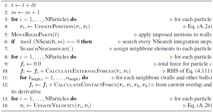
|
|
Algorithm. 9 Solve DEM function algorithm. These operations performed at every DEM time step. |
The equation of motion of the particles Eq.~4.1 must be modified to take into account the contact forces, as
|
|
(A.1) |
where runs over all the neighbouring particles, over all neighbouring triangular rigid walls, and where the binary parameter is introduced to easily turn off inter-particle interactions as required (such as in Section 4.7.8). The force is only actually computed if the neighbouring wall or particle center falls within the ball centred at the target particle's center and with radius equal to the search radius. The search radius is defined as the particle radius plus a tolerance that is tuned to optimize the computational cost. Such optimal cost is to be found as an ideal balance between the cost of running the search algorithm at every time step and having a larger number of neighbours per particle as a result of the enlarged search tolerance; see Section A.2.
A.1.1 Contact model
The contact model is the rheological model that relates the kinematics of a contacting pair with the force and moment between both particles involved (a plane can be seen as a degenerate particle). The kinematics in the DEM contain a number of subtleties that we will not cover here, but they can be roughly characterized by the evolution of three degrees of freedom (DOFs): the instantaneous values of the indentation and its derivative (normal motion; one DOF) and the complete history of the relative motion projected onto the plane that passes through the contact point and is orthogonal to the line joining the particles' centres (tangential motion, two DOFs).
Our contact model includes a Hertzian spring-dashpot model with no sticking [287] for the normal motion, with the particularity of having a constant coefficient of normal restitution (COR). This contact element is characterized by a spring constant and the COR. The tangential motion employs a Deresiewicz–Mindlin spring-dashpot model connected in series with a frictional element, characterized by a friction coefficient () (where and identify the material of the two particles involved) in addition to the tangential spring constant and a tangential dissipation coefficient.
The model was proposed by Thornton et al. [343], see also [64]. The COR is the ratio between the impact incident normal velocity (denominator) and the normal velocity immediately after contact (numerator), and is generally bounded between zero and one. It is a useful, engineering parameter to characterize the amount of energy dissipated by the impact of a given material. However, it must be kept in mind that the assumption of it being independent of the incident velocity is actually not entirely correct [210] and so the COR is not, strictly speaking, a material parameter, but only approximately so.
A.1.2 Time integration Scheme
To solve Eq.~4.1 (together with a suitable initial condition ), we can use a finite difference scheme. Several options are possible but we have run our simulations using the a version of the two-step Adams–Bashforth scheme, which has been extensively tested. The difference equations read as follows:
|
Where is the total force minus the terms proportional to the acceleration of the particle in the added mass force, which is treated implicitly by increasing the mass of the particle by . This two-step scheme can be started with the analogue, first step version of the same algorithm. A similar algorithm is used for the integration of the angular motion.
A.2 Scales
The introduction of DEM in point-particle methods implies that a new, (short) time scale is being resolved: the contact time scale. First of all, the fundamental reason 1 for introducing the DEM method in the first place is that collisions are regarded as playing a non-negligible role in the simulation. Therefore, it is always necessary to ensure the non-penetrability of the spheres through one another and, often, also through the walls.
The large majority of DEM simulations employ a contact model composed of an elastic element arranged in parallel with a dissipative element, commonly of viscous nature. This kind of arrangement is known as a spring-dashpot model. The role of the dissipative element is to ensure that a correct amount of energy is lost at each impact, since no real (macroscopic) system is perfectly elastic.
The energy-dissipating mechanism is in principle beneficial from the long-term numerical stability, since it helps to control energy build-ups, although it might also have the opposite effect in some situations, since dissipative contact models often place stronger limitations in the critical time step for numerical stability.
In any case, the intensity of the dissipation element cannot in general be tuned for numerical reasons, since the amount of energy dissipated at each impact is a crucial physical aspect that determines the macroscopic behaviour of the system, specially in collisional regimes (the motion is mostly formed of a succession of collisions alternated with contact-less, ballistic motion).
On the other hand, the action of the elastic element is typically less constrained by the physics. In many DEM simulations, specifically those dealing with moderately dense to disperse regimes, the role of the elastic element can be summarized as
- ensuring that sufficient repulsion is achieved in all circumstances to avoid excessive penetration and
- ensuring the separation of scales, in time and space, between those dynamic scales associated with free flight and those associated with the process of rebound.
Note that, in disperse simulations, it is often not relevant to resolve the actual rebound process with accuracy. In fact, in these situations the process is resolved only as a method to obtain a robust numerical technique, just as any penalty model in contact mechanics.
A.2.1 Choosing the time step size
The selection of a suitable time step is crucially important in any DEM simulation, since it has a proportional impact in the numerical cost of the simulations. As in any finite difference calculation, one would like to select the time step based on the required accuracy, so as to minimize the total number of time steps. However, the choice is also restricted by the need to preserve numerical stability and accuracy, which are both always conditional to the size of the time step, that must be kept small enough.
The analytical calculation of the time step can be attempted in some cases, mostly using approximations such as the linearisation of the nonlinear force models. However, such calculations are too complex in practice or lead to excessively rough estimates of little practical value. We base our choice of the time step on experience, often requiring a certain number of iterations in order to attain a good compromise between accuracy and cost.
Nonetheless, we do not proceed blindly, but actually apply a criterion that we next describe and that will also provide an argument to explain the high computational demands of this numerical approach. Our criterion is based on the following considerations:
- The smallest scales represented in our simulations correspond to the contact dynamics, and consequently it is the contact that dictates the maximum allowable time step, not the interactions with the fluid (only the added mass force, has a response time at a comparable time scale, but we are treating it implicitly).
- As discussed above, the stiffness of the contact model is considered a numerical parameter that can be softened to increase the critical time step for numerical stability. This practice is acceptable as long as the time scale of the contact is still properly separated (see [272] for a discussion on the issue of scales separation) and that the maximum indentations remain small, so as to not significantly affect the packing configuration and avoid going through obstacles.
- The contact must be properly resolved to avoid excessive numerical errors and spurious energy creation. This is guaranteed by dividing the contact duration in, at least 15, to 30 steps, depending on the numerical scheme.
According to this, we thus must first calculate the minimal expected contact duration. In order to do that, we may use the formula that can be found in [64] (see also [10]), valid for Hertzian contact. For Hertzian contact laws, the contact duration decreases with the impact velocity and thus the worse-case scenario is the largest estimated impact velocity. Once we have the minimal expected impact duration, we divide it into a large enough number, say, fifteen, and apply a security factor to further reduce it. We have observed that using this technique leads to robust estimations of the optimal time step with a limited need for trial-and-error.
(1) In absolute rigour, there exists the possibility of using the technique, almost unaltered, to simulate other types of close-range interactions, e.g.electric fields, that might not require strict impenetrability and for which the present discussion should be modified. These however fall out of the scope of the present work.
A.3 Wear
It would be interesting to predict the level of wear on the different surfaces of the drill bit under the repeated impact of the steel particles. While a quantitative prediction is certainly challenging, we believe there is a potential for the prediction of relevant qualitative trends, such as:
- the location of intense wear concentrations
- the sensitivity of the wear spread pattern upon changes in the design and operation parameters
- the identification of unexpected wear mechanisms
- the classification of frictional wear versus impact wear regions
We have implemented a simple wear model to illustrate these points. During the contact of a particle against a wall, an impact wear () contribution is calculated according to
|
|
(A.3) |
where is the normal relative velocity between the particle and the triangular surface. This quantity is then divided by the face area and distributed to the nodes using the triangle's shape functions. Note that while the factors in Eq.~A.3 surely contribute to the wear, their powers have been arbitrarily set to one for simplicity. A realistic model would require further investigations and is thus left for future work.
A.4 Analytic tools
Taking advantage of the object-oriented philosophy of Kratos Multiphysics, we have extended the notion of the discrete element to a generalized analytic discrete element. This type of element is designed to collect information during a simulation by increasing its associated data-structures in a trade-off of information vs. computational efficiency.
The key concept is to allow a (small) proportion of the discrete elements to be marked as analytic, behaving as the discrete element they generalize but performing a few extra operations and recording a few extra data. These discrete elements are constantly monitored by an external process that collects the information stored in each of the analytic elements, ignoring the rest. The concrete data stored in the data structures associated with these discrete elements are best understood by example. Here we give a brief account of two variants that we have implemented in our code.
A.4.1 Analytic particles
The analytic particle is a discrete element that interacts exactly identically with the rest of the particles but that keeps a record of the impact data associated with the contacting neighbours at a given time step. This means that the information is only related to a specific time step and thus must be collected at every time step or else it is lost. This design requires an operation to be added to the DEM solution with the same frequency as the DEM solution itself, but is only (relatively speaking) costly if the proportion of analytic particles is comparable to the total number of particles in the domain. The information collected from all the particles is stored in a database for later analysis. We use HDF5 files to store the information.
The reason of this design is to keep the data structures associated to the discrete elements as small as possible, so as to make the most out of the available cache. Having very heavy particles would result in extremely slow computations overall, spoiling the efficiency of the program. By limiting the total number of possible simultaneous impacts to a few (in our case, only four), the data structures are kept at a fixed size, avoiding allocation/deallocation on the fly. Note that it is extremely unlikely that more than four impacts occur at exactly the same time step.
The precise information kept per impact may vary, but a useful combination is to keep the impact velocity (normal and tangential to the particle surface), the ID of the other particle and the positions at the moment of impact. This information can be used in simulations to keep track of the impact frequency and violence [183] and other interaction such as chemical exchanges etc.
A.4.2 Analytic surfaces
By counting the triangular rigid faces as DEM elements too, one can generalize them in a similar way as we have explained with analytic particles. Such analogous surfaces could be used to track impact locations and wear [373] etc. But we have devised another type of analytic surface with the particularity of not affecting the contacting particles. Instead, these surfaces make measurements of the particles as those traverse them. This allows to measure fluxes of particles. The versatility of the DEM rigid faces is inherited by these flux-measuring particles, that may be meshed to cover any complicated cross-section. The information is again stored in appropriate HDF5 files for posterior analysis.
Appendix B. Quadrature substepping formulas
Daitche's method
Formulas Eq.~3.27 and Eq.~3.28 were given in Daitche [89]. A general formula was also derived in the same work which, it was claimed, contained Eq.~3.27 and Eq.~3.28 as special cases. This formula reads
|
|
(B.1) |
where is a function that returns the boolean truth value of the expression it evaluates (i.e., for true statements and otherwise) and where
|
|
(B.2) |
and where is the Lagrange polynomial that is equal to one at and zero at the remaining points in .
According to our calculations however, the direct application of Eq.~B.1, together with Eq.~B.2, does not in fact yield Eq.~3.28 for as it should. The origin of this inconsistency can be traced back to the way in which the interpolation points are positioned around a generic interval (Note that the notation in Daitche [89] was instead ), which was fixed according to different rules for the generic case and for the special cases in [89]. The derivation of Eq.~B.1 starts by considering the polynomial interpolation of in Eq.~3.2 with Lagrange polynomials in the interval . Daitche takes
|
|
(B.3) |
Which, particularized to order two () reads
|
|
(B.4) |
Figure 82 depicts the interpolation polynomials , and . In full line are represented the segments that are actually used for interpolation in . Fig. 83, meanwhile, depicts the interpolation term weighed by showing that its support is . In other words, this interval is the domain of influence of for the quadrature.
![Interpolation of f in a generic, away-from-the-boundary interval [ti, ti+1], according to the general formula proposed by [89].](/wd/images/thumb/e/ee/Draft_Samper_307425316-monograph-picture-57b127.png/400px-Draft_Samper_307425316-monograph-picture-57b127.png)
|
| Figure 82: Interpolation of in a generic, away-from-the-boundary interval , according to the general formula proposed by Daitche [89]. |
![Support of the interpolands weighed by f(ti), according to the general formula proposed by [89].](/wd/images/thumb/0/0f/Draft_Samper_307425316-monograph-picture-0e70d6.png/400px-Draft_Samper_307425316-monograph-picture-0e70d6.png)
|
| Figure 83: Support of the interpolands weighed by , according to the general formula proposed by Daitche [89]. |
We are going to show that, for second order, the interpolation scheme shown in Figs. 82 and 83 cannot lead to Eq.~3.28. Indeed, let us look at the central piece, i.e.for .
|
|
(B.5) |
Using , the formula becomes
|
|
(B.6) |
Now, remembering that is the coefficient of in the overall interpolation (see Eq.~3.26), it is clear that, according to Fig. 83, the influence of should be restricted to , and not to as in Eq.~B.6. This statement alone proves our claim without resorting to the a full calculation using the formula in Eq.~B.1. Our calculations show that however, this problem does not appear for order one or three. The reason is simple: Daitche chose to place the interpolating points as close as possible to the interval . For odd-order polynomials (even number of interpolation points), there arises a unique solution; i.e.a symmetric configuration with the interval in the middle. On the other hand, for even-order interpolations there are two possibilities: one having one more point to the left of the interval and the other having one more point to the right. The first option is implemented when using B.2. We propose to replace this equation by
|
|
(B.7) |
which implements the alternative option, that is, to have one more point to the right of the interval. Note that this formula is equivalent to B.2 for odd-order cases, while it moves one interval to the right the value of for the even-order ones (when possible, that is, away from the present-time boundary). Our calculations show that this solves the problem and that indeed Eq.~B.1, with the new definition of , holds and as special cases. Figs. 84 and 85 display the corrected configuration, consistent with Eq.~B.1 with Eq.~B.7 and, in particular, with Eq.~3.27 and Eq.~3.28.
![Interpolation of f in a generic, away-from-the-boundary interval [ti, ti+1], according to the corrected formula](/wd/images/thumb/a/a5/Draft_Samper_307425316-monograph-picture-055248.png/400px-Draft_Samper_307425316-monograph-picture-055248.png)
|
| Figure 84: Interpolation of in a generic, away-from-the-boundary interval , according to the corrected formula |
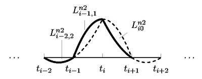
|
| Figure 85: Support of the second-order interpolands weighed by , according to the corrected formula |
First Order
The first-order interpolation polynomials are illustrated with full generality in Fig. 86. In order to compute the formula for , we remember that plays the role of the in the quadrature formula Eq.~3.26. Thus, only the Lagrange polynomial that are equal to one at contribute to this coefficient. Fig. 87 displays the different variations of the support of these polynomials. Let us calculate to illustrate the calculation of the different pieces of . The coefficient multiplies (see Eq.~3.26) and so we can rely on Fig. 87 to right
|
|
(B.8) |
so
|
|
(B.9) |
Similarly the rest of pieces are calculated, yielding the general formula Eq.~3.29.
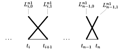
|
| Figure 86: Interpolation of . The distance between successive points is , except for the pair and , in which case it is . |

|
| Figure 87: Support of the first order interpolands |
Second Order
We will illustrate the calculation of the modified formulas by considering two cases: the central piece of the functions, that is, the analogue of Eq.~B.5 with a shortened last interval, which is only affected by the modified argument of the kernel; and the piece corresponding to and , representative of the formulas affected by the modification of the interpolation polynomials. The rest of the formulas are obtained similarly and only the final results will be included for the sake of brevity. We will proceed without resorting to the general formula Eq.~B.1. Instead, it is sufficient to refer to Fig. 85. The contribution of to the total integral is given by
|
|
(B.10) |
Substituting the formulas for the Lagrange polynomials and using and , we obtain
|
|
(B.11) |
Where now Eq.~B.5 is recovered for .
Let us now turn to the case where not only the kernel's argument changes, but also the definition of the interpolation polynomials. The case and requires the consideration of the situation displayed in Fig. 88. The general interpolation scheme has to be modified to avoid requiring points outside the domain (in this case future values). The contribution of is given by
|
|
(B.12) |
And again, substituting the formula for and using
|
|
(B.13) |
which again, for agrees with Eq.~3.28. Similar calculations can be performed for the rest of the cases, yielding the general expression Eq.~3.30.
![Interpolation of f at the interval [tₙ₋₂, tₙ]. The distance between tₙ₋₁ and tₙ is ϕh.](/wd/images/thumb/1/1f/Draft_Samper_307425316-monograph-picture-42a1df.png/400px-Draft_Samper_307425316-monograph-picture-42a1df.png)
|
| Figure 88: Interpolation of at the interval . The distance between and is . |
Appendix C. Alternative expression for the history force
We will first proof the relationship for kernels that are bounded in . We have that
|
|
(C.1) |
Now, when is not defined at , as in the case of the Basset kernel, the derivation above must be altered. We proceed by constructing a sequence of kernels that limit at the singular kernel to derive an analogous result. Consider
|
|
(C.2) |
where is a positive integer. The sequence of for all positive integers converges pointwise to the desired kernel . The result we are after will easily follow for if we can move the limit sign from the integrand on the LHS expression in Eq.~C.1 to outside the derivative, as we will show. Note that we are not interested in validity of the formula at exactly , since the impulse due to this infinite value at the initial time is zero anyway. Thus, mathematically, we want to show that for any
|
|
(C.3) |
First, the limit can me moved outside the integral by the Dominated Convergence theorem. All we must prove is that there exists an integrable function that is greater or equal to all the integrands in the sequence. But
|
|
(C.4) |
and the RHS is an integrable function, because
|
|
(C.5) |
On the other hand, to show that the limit can be moved outside the derivative as well, we use the following theorem [337, Theorem 3.7.1]:
Theorem 2: Let define a sequence of differentiable functions in a closed interval , for , and let be the corresponding sequence of derivatives, also defined in . Suppose that converges uniformly to some function , also defined in . Suppose also that there exists a point where the limit exists. Then converges uniformly to a differentiable function , and its derivative is .
We want to apply the theorem to the sequence of functions
|
|
(C.6) |
where is an arbitrary number in . We have already shown that
|
|
(C.7) |
To particularize Theorem 2 to these choices of and it is enough to show that the following hold:
a) Each is differentiable in . b) There exists a in , such that
|
|
(C.8) |
- exists.
c) The sequence converges uniformly to some function, , defined in .
The requirement a) follows immediately by the differentiability of the integrands. The requirement b) follows from the existence of the Basset force of all . Finally, let us consider
|
|
(C.9) |
which tends to zero as and tend to zero (assuming the derivative of to be well behaved). So the sequence is uniformly Cauchy and, thus, uniformly convergent to some function , defined in . We have proven that c) also holds. We can now apply Theorem 2 and write
|
|
(C.10) |
for all , where in the last equality we have used the Dominated Convergence theorem again to move the limit under the integral sign.
In summary, we have proved that the formula is valid in an interval , as long as ; thus proving Eq.~3.3, also for the Basset kernel.
Appendix D. Error bound for the kernel approximation
Let us define
|
|
(D.1) |
We want to establish an upper bound for Eq.~3.20. Ignoring the constant , we have that the RHS of this equation is
|
|
(D.2) |
Applying the change of variables , we obtain
|
|
(D.3) |
where and
|
|
(D.4) |
with defined as
|
|
(D.5) |
and
|
|
(D.6) |
In other words, is obtained from by substituting all the by their normalized counterparts. Now, from Eq.~D.3 and Eq.~D.1 we can immediately write
|
|
(9.7) |
where we have changed the dummy integration variable back to .
Appendix E. Quadratic character of the I2tH problem
In this Appendix, we outline the quadratic character of the minimization problem when bound is taken as the cost function. The values of bound must be given and we represent them by in as
|
|
(E.1) |
The kernel error with respect to can be written as
|
|
(E.2) |
Thus, the first term of bound can be expressed, using Einstein notation, as
|
|
(E.3) |
By defining the design variables as , the matrix, the vector and as
|
|
(E.4) |
the first term of is readily rewritten in matrix notation, as
|
|
(E.5) |
Similarly, the second term of has the following form
|
|
(E.6) |
Again defining matrix, the vector and as
|
|
(E.7) |
The second term of the bound can be compactly expressed as
|
|
(E.8) |
Collecting the first and the second terms, we obtain the final expression for the bound
|
|
(E.9) |
which stands for a standard quadratic minimization as
|
|
(E.10) |
where and are defined as and . Note that is suppressed from the expression since it does not play any role in the minimization problem.
Appendix F. Optimal ai and ti values
We provide the optimal and for each of the cost functions (Table F.1) and (Table F.2). Note the increasing distance between successive values, as was assumed by Hinsberg et al. [353]. Note also that for we obtained .
| 1.046347992 | 1.581186674 | 0.566192817 | 0.717656182 | 0.440072204 | 0.482318894 | 0.374397988 | 0.365083559 | 0.3450551877 | 0.3227320427 |
| 0.864298391 | 8.925153279 | 0.538287204 | 3.324763126 | 0.421322343 | 1.820334739 | 0.3762685526 | 1.4017593843 | ||
| 0.807797346 | 38.928376132 | 0.517872275 | 11.809488351 | 0.4383511621 | 7.3543952717 | ||||
| 0.761539469 | 127.109159354 | 0.5502868981 | 52.9058339347 | ||||||
| 0.7701813938 | 699.4337431732 | ||||||||
| 0.3227460255 | 0.2894856389 | 0.2931405176 | 0.2413624327 | 0.2718360249 | 0.2192620346 | 0.2570818336 | 0.1878604572 | 0.2520642358 | 0.1878604572 |
| 0.3446901326 | 1.1312690586 | 0.3053190176 | 0.8199848671 | 0.2685924185 | 0.662026818 | 0.2610118588 | 0.5420260992 | 0.254913066 | 0.5306382498 |
| 0.3924441164 | 5.1207861657 | 0.3394616674 | 3.0838532791 | 0.2871214552 | 2.0706383247 | 0.2799238451 | 1.6534881587 | 0.2638832071 | 1.5524873935 |
| 0.471576099 | 29.6345412934 | 0.3924532926 | 13.8047974118 | 0.3249589764 | 7.2825402363 | 0.3051985477 | 5.5204876302 | 0.2666445191 | 4.6517443725 |
| 0.5990063177 | 256.64908268 | 0.4794140412 | 80.9779742728 | 0.3805886345 | 31.0062809826 | 0.3418149337 | 20.8847203692 | 0.2806268115 | 14.2413555446 |
| 0.7695849793 | 4254.1241751139 | 0.5546383969 | 696.8320792921 | 0.4469592071 | 169.6857783353 | 0.3892337642 | 93.9005719593 | 0.344914608 | 50.7413819742 |
| 0.6207864425 | 6133.2449027098 | 0.5474439544 | 1226.001409491 | 0.4655655296 | 532.1532341216 | 0.4566204962 | 263.7561507819 | ||
| 0.7637048975 | 17271.9375778519 | 0.6107696402 | 4683.3937018005 | 0.5663046247 | 2146.211201895 | ||||
| 0.784623916 | 93277.7129340798 | 0.6253574036 | 26744.590748687 | ||||||
| 0.6932526975 | 348322.670028861 | ||||||||
| 0.9384724434 | 1.4300340551 | 0.5470597552 | 0.6666835275 | 0.430797005 | 0.4521461414 | 0.3714051613 | 0.3505056162 | 0.3335736291 | 0.2904610289 |
| 0.8449767491 | 8.3424872407 | 0.5319402016 | 3.0597097311 | 0.4221306386 | 1.7525741335 | 0.3629331173 | 1.203691574 | ||
| 0.8046471493 | 36.769402335 | 0.5248827638 | 11.6528756138 | 0.4197252519 | 5.9370324806 | ||||
| 0.7814317902 | 136.8864124598 | 0.520201698 | 39.1450598115 | ||||||
| 0.7661038702 | 452.8226228869 | ||||||||
| 0.3065928563 | 0.2504309713 | 0.2869667584 | 0.2229567355 | 0.2695926115 | 0.1998084724 | 0.2560766303 | 0.1826244466 | 0.2467020831 | 0.1711374102 |
| 0.3243480187 | 0.9103056758 | 0.297777436 | 0.7379950193 | 0.2751628513 | 0.6094217589 | 0.2580812359 | 0.5231166336 | 0.2464749444 | 0.4695384557 |
| 0.3615932545 | 3.7204976994 | 0.3249218804 | 2.6583099103 | 0.2954155007 | 1.9746292865 | 0.2739535236 | 1.5665809982 | 0.2597178682 | 1.3336047234 |
| 0.418122689 | 18.2727422761 | 0.3631687423 | 10.9237321521 | 0.3228159111 | 7.0527307887 | 0.2950977014 | 5.0639463936 | 0.2773405882 | 4.038729849 |
| 0.5168085735 | 119.760302387 | 0.420482447 | 54.149026921 | 0.3602702642 | 28.6942745173 | 0.3224941082 | 18.0664363914 | 0.2995010019 | 13.2686834339 |
| 0.7551149413 | 1369.9016377844 | 0.5207711634 | 360.6375769122 | 0.4159293673 | 140.1890961279 | 0.3598005017 | 73.4054449448 | 0.3282822047 | 48.3505553197 |
| 0.7554318595 | 4254.1243411105 | 0.5121568839 | 911.2555045811 | 0.4151331109 | 357.9494752882 | 0.3678821811 | 202.2013044128 | ||
| 0.7402280446 | 10263.3419763251 | 0.5104760265 | 2319.7684648904 | 0.4276240337 | 1029.0899279619 | ||||
| 0.7348997012 | 25980.6116922192 | 0.5335800139 | 7177.8752909387 | ||||||
| 0.7652665389 | 93277.7373733731 | ||||||||
Apppendix G. FEM Discretization of the CFD-DEM equations
We provide in this appendix the developed expressions for the elemental matrices for both the Q-OSS and the Q-ASGS formulations.
G.1 OSS FEM discretization
Let us now perform the space discretization of the problem. Putting together the abstract expression of the variational problem, given by Eq.~4.50, with the bilinear form from Eq.~4.142, the RHS Eq.~4.143 and the stabilization terms from Eq.~4.144 we obtain
|
|
(G.1) |
Let us now substitute in the standard finite element discretization in Eq.~4.20, taking one term at a time, to construct the elemental matrices. The first term is:
|
|
(G.2) |
Introducing the shape functions in the integral above yields the following expression. Here and in similar developments later on, the integration domain and the volume differential will often be suppressed for the sake of conciseness.
|
|
(G.3) |
where the time derivative of the nodal values will in practice generate terms that will depend on the old values, which will be sent to the RHS.
The elemental contribution to be assembled to the global stiffness matrix is obtained by considering the contribution to the above integral due to the elemental domain and considering the nodes belonging to that domain and their corresponding shape functions. The elemental mass matrix corresponding to the element is as follows
|
|
(G.4) |
where
|
|
(G.5) |
where the and indices run through the element nodes. Let us now look at the elemental contribution of the next term, that is, the convective term
|
|
(G.6) |
The associated elemental matrix is given by
|
|
(G.7) |
where
|
|
(G.8) |
The next term is of the form
|
|
(G.9) |
The elemental matrix contribution due to the third term is thus
|
|
(G.10) |
where
|
|
(G.11) |
Let us now look at the fourth term.
|
|
(G.12) |
so the associated elemental matrix is
|
|
(G.13) |
with
|
|
(G.14) |
The next term is developed as follows:
|
|
(G.15) |
The associated elemental matrix contribution is therefore
|
|
(G.16) |
with
|
|
(G.17) |
The gradient viscous terms are of the form (for the fluid equation)
|
|
(G.18) |
And the associated matrix (now including the particle phase contribution)
|
|
(G.19) |
with
|
|
(G.20) |
The divergence type viscous terms are of the form
|
|
(G.21) |
The associated matrix is (now including the particle phase contribution)
|
|
(G.22) |
with
|
|
(G.23) |
Let us now expand the contribution of the stabilization terms. The first term that we will develop is the one of the form .
|
|
(G.24) |
The elemental contribution looks as follows
|
|
(G.25) |
where
|
|
(G.26) |
Let us now look at the term structurally similar to .
|
|
(G.27) |
The elemental contribution is as follows
|
|
(G.28) |
where
|
|
(G.29) |
We next look at terms of the form
|
|
(G.30) |
The corresponding elemental contributions read
|
|
(G.31) |
where
|
|
(G.32) |
We now turn to the terms of the form .
|
|
(G.33) |
The elemental matrix turns out to be
|
|
(G.34) |
where
|
|
(G.35) |
We now turn to the set of terms multiplied by . The first is of the form
|
|
(G.36) |
The corresponding elemental matrix is
|
|
(G.37) |
where
|
|
(G.38) |
The last term is of the form , which has already shown up i the viscous term. Therefore the elemental matrix contribution is
|
|
(G.39) |
with
|
|
(G.40) |
In order to complete the matrix formulation, it is necessary to expand the RHS terms also. Let us now do this, again, taking it term by term and neglecting second-order derivatives within the element domains. The first type of terms to be added are of the form , where is a constant vector (with regards to integration).
|
|
(G.41) |
The corresponding matrix contributions are
|
|
(G.42) |
where
|
|
(G.43) |
The second standard Galerkin term is of the form .
|
|
(G.44) |
Therefore we have the following matrix contribution:
|
|
(G.45) |
where
|
|
(G.46) |
Let us now look at the stabilization terms. The first one is of the form
|
|
(G.47) |
Therefore, we have the following matrix terms
|
|
(G.48) |
where
|
|
(G.49) |
The last term multiplying is of the form .
|
|
(G.50) |
The corresponding matrix contribution is
|
|
(G.51) |
where
|
|
(G.52) |
There only remains to develop the the term multiplying either . It is of the form .
|
|
(G.53) |
Therefore we have the following matrix contribution
|
|
(G.54) |
where
|
|
(G.55) |
We will additionally compute the expression corresponding to the Neumann boundary terms:
|
|
(G.56) |
The matrix contribution is
|
|
(G.57) |
where
|
|
(G.58) |
Let us now assemble all these contributions as if only one element was present, so as to visualize the relationships between all the matrices.
|
|
(G.59) |
where the first terms on both sides LHS are the standard Galerkin contribution, while the second terms are the contribution of the stabilization terms.
G.2 ASGS FEM discretization
Next we derive the matrix contributions corresponding to the ASGS discretization, for the case of quasi-static subscales. The main difference with respect to the OSS method is the presence of the dynamic contribution in the stabilization terms on the LHS. This term can be developed into
|
|
(G.60) |
Let us now develop the finite element contributions corresponding to this expression, taking each term one by one. The first term is of the form
|
|
(G.61) |
The elemental contribution is therefore
|
|
(G.62) |
where
|
|
(G.63) |
The second term is of the form
|
|
(G.64) |
The elemental contribution in this case is
|
|
(G.65) |
where
|
|
(G.66) |
Finally, the RHS stabilization terms must be defined. Their structure is similar to those present in the OSS method, where only the constant vectors differ. The ASGS analogous matrix contributions are next listed
|
|
(G.67) |
where;
|
|
(G.68) |
|
|
(G.69) |
where; and
|
|
(G.70) |
|
|
(G.71) |
where
|
|
(G.72) |
Let us now assemble all the above elemental matrix contribution for the ASGS method
|
|
(G.73) |
Appendix H. Multicomponent theory fundamentals
H.1 The backward-coupled continuous problem
The theory of multicomponent flows can be understood as a generalization of (single-phase) continuum mechanics. The fundamental concepts defined in the latter are carried over in this generalization in a natural way. For this reason, a very concise summary of the most fundamental notions is next presented, also for the single-component case, so as to fix notation and terminology and facilitate the task of the reader unacquainted with the theory. In the exposition we mainly follow [109].
H.1.1 Single-component continuum theory: basic notions
Let the material body manifold describing the continuum be denoted as . A configuration is a differentiable map , where represents the classical affine Euclidean space of continuum mechanics. The motion of is a differential mapping, , defined by , defined, for each , as
|
|
(H.1) |
where the define a family of configurations parametrized by , to be interpreted as the time passed since some initial time. The Lagrangian description of the body motion is the differential mapping, , obtained as:
|
|
(H.2) |
where is the inverse of a configuration, referred to as the reference configuration, which is usually taken as
|
|
(H.3) |
In this case, the reference configuration is to be interpreted as a mapping between the points in body and their spatial positions at the initial time.
Balance of mass
We suppose the existence of an absolutely continuous function defined pointwise on , such that the mass measure is defined as
|
|
(H.4) |
where is any -measurable subset of .
The integral version of the postulate of balance of mass is
|
|
(H.5) |
The Dubois-Remond lemma implies its local counterpart, e.i.,
|
|
(H.6) |
Balance of momentum
Its integral version can be written as
|
|
(H.7) |
where (omitting explicit mention to functional dependences and volume integration domains, both coinciding with )
|
The point-wise expression of the momentum balance is:
|
|
(H.12) |
Balance of moment of momentum
Its integral version can be written as
|
|
(H.13) |
where (for non-polar materials with no momentum surface sources) and ting explicit mention to functional dependences and volume integration domains, both coinciding with )
|
where is the axial vector of tensor , i.e..
The point-wise expression of the moment of momentum balance is:
|
|
(H.18) |
Balance of energy
Its integral version can be written as
|
|
(H.19) |
where
|
The point-wise expression of the energy balance is:
|
|
(H.23) |
H.1.2 Multi-component continuum theory: basic notions
A sequence of body manifolds , (bodies) are considered. A motion is defined for each component:
|
|
(H.24) |
where each family of configurations is analogous to the corresponding families introduced for single-component motions.
Balance of mass
A mass measure is defined for each component:
|
|
(H.25) |
where is density-like variable defined as
|
|
(H.26) |
where each is the volume fraction, a continuous field with values in and such that
|
|
(H.27) |
The integral version of the postulate of balance of mass is
|
|
(H.28) |
The Dubois-Remond lemma implies its local counterpart, e.i.,
|
|
(H.29) |
Balance of momentum
Its integral version can be written as
|
|
(H.30) |
where (omitting explicit mention to functional dependences and volume integration domains, both coinciding with )
|
where analogously to Eq.~H.26 we define
|
and where is the momentum exchange with other components. The point-wise expression of the momentum balance is then:
|
|
(H.36) |
Balance of moment of momentum
Its integral version is expressed as
|
|
(H.37) |
where, for non-polar materials with no momentum surface sources) and omitting explicit mention to functional dependences and volume integration domains, both coinciding with
|
The point-wise expression of the balance of moment of momentum is:
|
|
(H.41) |
Balance of energy
Its integral version can be written as
|
|
(H.42) |
where
|
and where is the source to component due to the interaction with other components.
The point-wise expression of the energy balance is:
|
|
(H.46) |
H.1.3 An important particularization of the balance equations
Let us consider there are only two phases: one is a continuous phase, composed of an incompressible continuous, incompressible fluid and the other is a dispersed phase, also assumed to be incompressible. Let us further assume that the body forces are the effect of a constant gravity field . Let the subindex denote the continuous fluid phase while denotes the particles phase. The mass, momentum and energy local balance equations may be written as
|
where denotes the contribution of momentum from the fluid to the particles. Obviously, this set of differential equations must be accompanied by the restriction:
|
|
(H.53) |
at all points in the domain of definition.The momentum equations may, equivalently, be written, following what is done in [182] as
|
where a buoyancy force has now been subtracted from , such that may be refereed to hydrodynamic force density. Derksen and Sundaresan [97] have called this term the local fluid-particle interaction force per unit volume, as it is caused by effects of a small scale nature, as opposed to the larger-scale varying term .
Eqs.H.47 and H.52 are sometimes taken as an axiom (postulational approach, see, e.g. [359]), but they may also be obtained from single-phase continuum balance equations for each phase through averaging [109]. Several averaging methods have been devised for this matter, including time [179], volume [8] and ensemble averages [109], among others. All these approaches arrive at equations that conform to these (although the physical interpretations of the quantities involved are of course quite diverse). In order for the presented equations to define (along a suitable set of boundary conditions) a well-posed problem, closures (extra equations) must be provided for several of their terms, since the present number of scalar equations (1 + 1 + 3 + 3 + 1 + 1 = 11) is less than the number of scalar variables (33).
H.1.4 Filtering of a particle-laden flow
In this subsection we slightly generalize the equations in Anderson and Jackson [8] to obtain the analogous relations for a more general averaging procedure. We recast the problem in the language of filters, common in the field of turbulence modelling [303], unifying space and time averages in the same framework. We will focus on the problem of isotropic filters, ignoring for the moment the problem of boundaries, although this is also the case in [8].
The filtering operation is the convolution of a kernel function with the field that one wants to smooth out. We will from the start assume a kernel function defined in is of the following form , where are positive, monotonically decreasing functions that vanish at infinity. A necessary condition for the operation to yield a meaningful description of the system, it is required that the smallest characteristic scales , of the flow are such that there is separation of scales, that is
|
|
(H.56) |
where and are the characteristic scales for the variation of and respectively. Anderson and Jackson [8] propose the following condition for the definition of
|
|
(H.57) |
where is the ball centred at zero with radius . And, by analogy, one can take
|
|
(H.58) |
as the condition that defines .
Our goal is the construction of averaged fields, such as the ones reviewed in Section H.1.2. We do so by applying the following filter to any tensorial quantity of arbitrary order
|
|
(H.59) |
where is either (particles) or (fluid); is the indicator function of the spatial configuration of the component . For instance, is zero inside the particles and zero everywhere else.
Note that for , the Dirac delta function, we would recover the usual volume averaging, while would yield the usual time averaging.
This filter allows to define the volume fraction fields as
|
|
(H.60) |
Using the volume fractions, we can define the component-averaged quantities as follows
|
|
(H.61) |
Note that we choose to define the component-averaged variables as derived quantities in the theory, rather than in [8], where they are taken as fundamental. This allows us to define the averaging procedure as a filter and avoids the undefinition of the averaged variables in the regions of the domain where the volume fractions vanish.
Now, in order to derive the conservation equations, we first derive two relations involving derivatives of the filtered quantities.
|
|
(H.62) |
where is the subset of where we find the component and where in the third last equality we have used Reynolds' transport theorem and where the last approximate identity is true far from the boundaries. The second identity is (take to be an arbitrary component of )
|
|
(H.63) |
where in the last equality we have used Gauss' theorem.
The next step is filtering both sides of the equation of interest. Let us apply it to the mass conservation and momentum conservation equations. In order to do so, we must imagine that the values of all the fields extend throughout the domain (e.g.the fluid velocity is defined inside the particles). The value chosen for the fields in this extension is not important, since the indicator function weighs them with zero. A simple possibility is to set them to zero in the extended areas. Having done this, we can equate the filtered versions of both sides of the conservation equation in question. Let us start with the mass conservation equation
|
|
(H.64) |
where we have used Eq.~H.63 in the first equality and Eq.~H.62 in the second. Note that this expression can alternatively be written as
|
|
(H.65) |
which has the form of Eq.~H.29 for constant density.
For the momentum equation, let us first, using Eq.~H.62 we have
|
|
(H.66) |
While using Eq.~H.63 we have
|
|
(H.67) |
Then, filtering the LHS of Section H.1.1 and assuming a constant density we obtain
|
|
(H.68) |
The second term above is not defined in terms of the filtered variables and it i convenient to decompose it further to isolate the unclosed quantities. In order to do so, the next step, following [8], is to decompose into a sum of an average and a sub-scale component, like this
|
|
(H.69) |
In [8] this decomposition is performed at each point in the domain, and then the filtering operation is performed, leading to
|
|
(H.70) |
The approximation above is justified by taking the first averaged quantity out of the average and neglecting the second term above, based on the separation of scales.
Another option is to write
|
|
(H.71) |
Where some of the dependencies have not been made explicit for the sake of conciseness. Now the approximations have been avoided by splitting the field into the average evaluated at the target point. The price to pay is the introduction of the field , which depends on four variables and describes the difference of the unfiltered field with respect to the filtered field, where filter point and point of measure are independent.
In any case, applying the above decomposition to Eq.~H.68 we obtain
|
|
(H.72) |
which, using Eq.~H.65, can be simplified to
|
|
(H.73) |
where are to be interpreted as the components of the second term in the RHS of equation Eq.~H.70 or Eq.~H.71, depending on the approximation one wishes to work with. Models for this quantity are to be provided to express it in terms of the averaged variables.
Now let us apply the filter to the RHS Eq.~H.12. The result is
|
|
(H.74) |
The first term above offers no difficulties, especially when taking as the constant acceleration due to gravity. We can apply Eq.~H.63 for the second term, which yields
|
|
(H.75) |
Now, we may identify the first term as the average force per unit volume on the particles. The second term can be approximated as
|
|
(H.76) |
That is, by equating the average stress due to the interface force exchange on the particles with that on the fluid. Note that this is reasonable taking into account the small size of the particles. Note that this reasoning concentrates the approximation step in this single last operation, in contrast to what is done in [8]. The final form of the filtered momentum balance is (using Eqs.~H.73-H.76)
|
|
(H.77) |
where
|
|
(H.78) |
and where is the average force per unit volume felt by the disperse phase due to the surface momentum exchange with the continuous phase. Both quantities will need to be modelled, since no analytic closed model exists. Ignoring the stress tensor for a moment, note that is of the form of Eq.~H.49 as is readily seen after identifying the subindex with , with and removing the averaging notation. However, the same analogy does not appear to work with the stress tensor, since one would expect to identify with . Though, formally, the analogy works rather with it corresponding to above.
In reality, the difference appears from an alternative decomposition of the different contributions. Note that if one takes Eq.~H.74 and reinterprets the second term in this equation as , one obtains a perfect term-to-term match with Eq.~H.49. However this partition is arguably less consistent than the former. This is because this second interpretation is using the filter with the surface contributions and so one is mixing volume averages with surface averages. In the former interpretation it is the volume-averaged momentum exchange between phases that is used, which generates the two terms in Eq.~H.75. The first of these two terms is the consistent (volume-averaged) interpretation of the momentum exchange between phases, while the second is absorbed, after the single approximation Eq.~H.76 into the second term of Eq.~H.49, as it is of the same form. The nature of this difference has not been always recognized as such. See, for example, the oft-cited paper [355]. See also [182] for a well-exposed argument about the often wrongly interpreted differences between two-phase models for the balance equations.
In the end, it will be necessary to provide closures for both the stress tensor and the momentum inter-phase exchange terms, so the relative merit of each decomposition will depend on the adequacy of the closure model provided. Thanks to the analysis of the averaging procedure, we now have a more explicit meaning for each of the referred terms.
Document information
Published on 31/01/19
Submitted on 31/01/19
Licence: CC BY-NC-SA license
Share this document
claim authorship
Are you one of the authors of this document?
![Number of particles associated to cubic domains for a fixed proportion of volume occupied by the particles (1x10⁻¹) as a function of the equivalent side length of the domain. The curves corresponding to different numbers of particles are included, as well as the upper limit sizes for clay, silt and sand, as representative granular materials. The scattered points correspond to different industrial application examples: coal, salt and nuts pneumatic conveying (volume per linear meter for typical pipe diameters); fluidized bed experiments of [143], showing the different Geldart categories; and catalytic cracking (FCC) for the production of gasoline.](/wd/images/thumb/4/45/Draft_Samper_307425316_7710_scales_DEM.png/510px-Draft_Samper_307425316_7710_scales_DEM.png)
