m (Cinmemj moved page Draft Samper 863111864 to Onate et al 2019a) |
|||
| (58 intermediate revisions by the same user not shown) | |||
| Line 1: | Line 1: | ||
| − | + | Published in ''Engineering Computations'' Vol. 18 (3-4), pp. 642-662, 2001<br /> | |
| + | doi: 10.1108/02644400110387190 | ||
==Abstract== | ==Abstract== | ||
| Line 27: | Line 28: | ||
{| class="floating_imageSCP" style="text-align: center; border: 1px solid #BBB; margin: 1em auto; width: 100%;max-width: 100%;" | {| class="floating_imageSCP" style="text-align: center; border: 1px solid #BBB; margin: 1em auto; width: 100%;max-width: 100%;" | ||
|- | |- | ||
| − | |[[Image:Draft_Samper_863111864-test-fig1.png| | + | |[[Image:Draft_Samper_863111864-test-fig1.png|400px|Deformation process of a solid]] |
|- style="text-align: center; font-size: 75%;" | |- style="text-align: center; font-size: 75%;" | ||
| colspan="1" | '''Figure 1:''' Deformation process of a solid | | colspan="1" | '''Figure 1:''' Deformation process of a solid | ||
| Line 201: | Line 202: | ||
where <math display="inline">{\boldsymbol N}</math> and <math display="inline">{\boldsymbol a}</math> are the shape function matrix and the nodal displacement vector, respectively. | where <math display="inline">{\boldsymbol N}</math> and <math display="inline">{\boldsymbol a}</math> are the shape function matrix and the nodal displacement vector, respectively. | ||
| − | ''The incremental secant stiffness'' expression is now obtained by substituting equations (4), (5), (8), (9), (10), (11) and ([[#eq-15|15]]) into ([[#eq-13|13]]) and collecting the terms depending on <math display="inline">{\boldsymbol \Delta a}</math> in the following form: | + | ''The incremental secant stiffness'' expression is now obtained by substituting equations ([[#eq-4|4]]), ([[#eq-5|5]]), ([[#eq-8|8]]), ([[#eq-9|9]]), ([[#eq-10|10]]), ([[#eq-11|11]]) and ([[#eq-15|15]]) into ([[#eq-13|13]]) and collecting the terms depending on <math display="inline">{\boldsymbol \Delta a}</math> in the following form: |
<span id="eq-16"></span> | <span id="eq-16"></span> | ||
| Line 241: | Line 242: | ||
|} | |} | ||
| − | In eq.(16) <math display="inline">{}^{t + \Delta t}{\boldsymbol f}</math> is the equivalent nodal force vector deduced from eq.(14) and <math display="inline">{}^t_r{\boldsymbol B}_L</math> is the first order strain matrix relating first order strain increments <math display="inline">{}_r e_{ij}</math> and nodal displacements <math display="inline">\Delta u_i</math>. The expression of this matrix can be found in <span id='citeF-13'></span>[[#cite-13|[13]]] and <span id='citeF-15'></span>[[#cite-15|[15]]]. | + | In eq.([[#eq-16|16]]) <math display="inline">{}^{t + \Delta t}{\boldsymbol f}</math> is the equivalent nodal force vector deduced from eq.([[#eq-14|14]]) and <math display="inline">{}^t_r{\boldsymbol B}_L</math> is the first order strain matrix relating first order strain increments <math display="inline">{}_r e_{ij}</math> and nodal displacements <math display="inline">\Delta u_i</math>. The expression of this matrix can be found in <span id='citeF-13'></span>[[#cite-13|[13]]] and <span id='citeF-15'></span>[[#cite-15|[15]]]. |
Equation ([[#eq-16|16]]) is a non linear system of algebraic equations relating the increment of forces with the displacement increments. Indeed this secant equation can be used as a basis for deriving different non linear solution schemes to track the load–displacement pattern <span id='citeF-13'></span>[[#cite-13|[13]]], <span id='citeF-14'></span>[[#cite-14|[14]]]. An alternative procedure for deriving secant stiffness expressions can be found in <span id='citeF-16'></span>[[#cite-16|[16]]]. | Equation ([[#eq-16|16]]) is a non linear system of algebraic equations relating the increment of forces with the displacement increments. Indeed this secant equation can be used as a basis for deriving different non linear solution schemes to track the load–displacement pattern <span id='citeF-13'></span>[[#cite-13|[13]]], <span id='citeF-14'></span>[[#cite-14|[14]]]. An alternative procedure for deriving secant stiffness expressions can be found in <span id='citeF-16'></span>[[#cite-16|[16]]]. | ||
| Line 257: | Line 258: | ||
|} | |} | ||
| − | Figure 2 shows schematically the difference between the incremental and total secant approaches. Further details can be found in <span id='citeF-8'></span>[[#cite-8|[8]]], <span id='citeF-13'></span>[[#cite-13|[13]]]–<span id='citeF-15'></span>[[#cite-15|[15]]]. | + | Figure [[#img-2|2]] shows schematically the difference between the incremental and total secant approaches. Further details can be found in <span id='citeF-8'></span>[[#cite-8|[8]]], <span id='citeF-13'></span>[[#cite-13|[13]]]–<span id='citeF-15'></span>[[#cite-15|[15]]]. |
<div id='img-2'></div> | <div id='img-2'></div> | ||
{| class="floating_imageSCP" style="text-align: center; border: 1px solid #BBB; margin: 1em auto; width: 100%;max-width: 100%;" | {| class="floating_imageSCP" style="text-align: center; border: 1px solid #BBB; margin: 1em auto; width: 100%;max-width: 100%;" | ||
|- | |- | ||
| − | |[[Image:Draft_Samper_863111864-test-fig2.png| | + | |[[Image:Draft_Samper_863111864-test-fig2.png|500px|Total (left) and incremental (right) secant approaches]] |
|- style="text-align: center; font-size: 75%;" | |- style="text-align: center; font-size: 75%;" | ||
| colspan="1" | '''Figure 2:''' Total (left) and incremental (right) secant approaches | | colspan="1" | '''Figure 2:''' Total (left) and incremental (right) secant approaches | ||
| Line 279: | Line 280: | ||
|} | |} | ||
| − | Using <math display="inline">{}^t_r {\boldsymbol K}_T</math> the standard iteration techniques for the computation of stability points in structures can be obtained. For instance, the standard Newton–Raphson method is written from eq.(16) as | + | Using <math display="inline">{}^t_r {\boldsymbol K}_T</math> the standard iteration techniques for the computation of stability points in structures can be obtained. For instance, the standard Newton–Raphson method is written from eq.([[#eq-16|16]]) as |
<span id="eq-21"></span> | <span id="eq-21"></span> | ||
| Line 292: | Line 293: | ||
|} | |} | ||
| − | In our work this theory was implemented for | + | In our work this theory was implemented for two-node truss elements and 8 node solid elements. The detailed form of all the relevant matrices can be seen in <span id='citeF-8'></span>[[#cite-8|[8]]], <span id='citeF-13'></span>[[#cite-13|[13]]] and <span id='citeF-15'></span>[[#cite-15|[15]]]. |
===2.2 Computing the equilibrium path=== | ===2.2 Computing the equilibrium path=== | ||
| Line 298: | Line 299: | ||
In order to trace the equilibrium path the load terms have to be scalable. For this purpose, the scalar load parameter <math display="inline">{}^t \lambda </math> is introduced. This parameter leaves the pattern of the external loads unchanged, only the size is varied (i.e. <math display="inline">{}^t{\boldsymbol f}={}^t\lambda {\boldsymbol f}_0</math>). | In order to trace the equilibrium path the load terms have to be scalable. For this purpose, the scalar load parameter <math display="inline">{}^t \lambda </math> is introduced. This parameter leaves the pattern of the external loads unchanged, only the size is varied (i.e. <math display="inline">{}^t{\boldsymbol f}={}^t\lambda {\boldsymbol f}_0</math>). | ||
| − | The arc–length method is commonly used to calculate equilibrium solutions for different loads and displacements. Therefore the equation defining the load increment is formally extended by one equation <math display="inline">f({}^t\lambda ,{\boldsymbol {}^tu})=0</math>, which determines the load parameter <math display="inline">{}^t \lambda </math>. A variety of different control equations can be found in the literature <span id='citeF-4'></span>[[#cite-4|[4]]], <span id='citeF-6'></span>[[#cite-6|[6]]]. The ones used here are stated below in equation ([[#eq- | + | The arc–length method is commonly used to calculate equilibrium solutions for different loads and displacements. Therefore the equation defining the load increment is formally extended by one equation <math display="inline">f({}^t\lambda ,{\boldsymbol {}^tu})=0</math>, which determines the load parameter <math display="inline">{}^t \lambda </math>. A variety of different control equations can be found in the literature <span id='citeF-4'></span>[[#cite-4|[4]]], <span id='citeF-6'></span>[[#cite-6|[6]]]. The ones used here are stated below in equation ([[#eq-22|22]]). |
| − | <span id="eq- | + | <span id="eq-22"></span> |
{| class="formulaSCP" style="width: 100%; text-align: left;" | {| class="formulaSCP" style="width: 100%; text-align: left;" | ||
|- | |- | ||
| Line 308: | Line 309: | ||
| style="text-align: center;" | <math>f({}^t\lambda ,{\boldsymbol {}^tu}) \; = \begin{cases} \qquad {}^{t+\Delta t} u_i - c & \mbox{ displacement control}\\ ({\boldsymbol u_m} - {}^t {\boldsymbol u})^T ({}^{t+\Delta t}{\boldsymbol u}-{\boldsymbol u_m})+( \lambda _m - {}^t \lambda )({}^{t+\Delta t}\lambda - \lambda _m) & \mbox{ normal plane} \\ \\ \sqrt{\|{}^{t+\Delta t}{\boldsymbol u} - {}^t {\boldsymbol u}\| ^2 +({}^{t+\Delta t}\lambda - {}^t \lambda )^2} - ds & \mbox{ cylindrical}\end{cases} </math> | | style="text-align: center;" | <math>f({}^t\lambda ,{\boldsymbol {}^tu}) \; = \begin{cases} \qquad {}^{t+\Delta t} u_i - c & \mbox{ displacement control}\\ ({\boldsymbol u_m} - {}^t {\boldsymbol u})^T ({}^{t+\Delta t}{\boldsymbol u}-{\boldsymbol u_m})+( \lambda _m - {}^t \lambda )({}^{t+\Delta t}\lambda - \lambda _m) & \mbox{ normal plane} \\ \\ \sqrt{\|{}^{t+\Delta t}{\boldsymbol u} - {}^t {\boldsymbol u}\| ^2 +({}^{t+\Delta t}\lambda - {}^t \lambda )^2} - ds & \mbox{ cylindrical}\end{cases} </math> | ||
|} | |} | ||
| − | | style="width: 5px;text-align: right;white-space: nowrap;" | ( | + | | style="width: 5px;text-align: right;white-space: nowrap;" | (22) |
|} | |} | ||
| Line 315: | Line 316: | ||
===2.3 Prediction of instability points=== | ===2.3 Prediction of instability points=== | ||
| − | The main criterion for existance of a critical point is that the tangent stiffness matrix <math display="inline">{\boldsymbol K}_T</math> becomes singular at the point. Mathematically this means that equation ([[#eq- | + | The main criterion for existance of a critical point is that the tangent stiffness matrix <math display="inline">{\boldsymbol K}_T</math> becomes singular at the point. Mathematically this means that equation ([[#eq-23|23]]) below has nontrivial solutions. |
| − | <span id="eq- | + | <span id="eq-23"></span> |
{| class="formulaSCP" style="width: 100%; text-align: left;" | {| class="formulaSCP" style="width: 100%; text-align: left;" | ||
|- | |- | ||
| Line 325: | Line 326: | ||
| style="text-align: center;" | <math>{\boldsymbol K}_T({\boldsymbol a}_c) \Delta{\boldsymbol a} \; = \; 0 </math> | | style="text-align: center;" | <math>{\boldsymbol K}_T({\boldsymbol a}_c) \Delta{\boldsymbol a} \; = \; 0 </math> | ||
|} | |} | ||
| − | | style="width: 5px;text-align: right;white-space: nowrap;" | ( | + | | style="width: 5px;text-align: right;white-space: nowrap;" | (23) |
|} | |} | ||
| Line 334: | Line 335: | ||
The singularity of the tangent matrix <math display="inline">{\boldsymbol K}_T</math> has some further consequences. The determinant of <math display="inline">{\boldsymbol K}_T</math> is equal to <math display="inline">0</math> in the critical point, furthermore the smallest eigenvalue is <math display="inline">0</math>. This can be stated mathematically as | The singularity of the tangent matrix <math display="inline">{\boldsymbol K}_T</math> has some further consequences. The determinant of <math display="inline">{\boldsymbol K}_T</math> is equal to <math display="inline">0</math> in the critical point, furthermore the smallest eigenvalue is <math display="inline">0</math>. This can be stated mathematically as | ||
| − | <span id="eq- | + | <span id="eq-24.a"></span> |
{| class="formulaSCP" style="width: 100%; text-align: left;" | {| class="formulaSCP" style="width: 100%; text-align: left;" | ||
|- | |- | ||
| Line 345: | Line 346: | ||
|} | |} | ||
| − | <span id="eq- | + | <span id="eq-24.b"></span> |
{| class="formulaSCP" style="width: 100%; text-align: left;" | {| class="formulaSCP" style="width: 100%; text-align: left;" | ||
|- | |- | ||
| Line 356: | Line 357: | ||
|} | |} | ||
| − | Many indirect methods for the computation of critical points use condition (24a) to determine their location on the equilibrium path. Nevertheless, in order to verify if a point indeed is a critical point these criteria can serve as test functions. Plotting <math display="inline">det {\boldsymbol K}_T</math>, the curve should become <math display="inline">0</math> at the critical point according to eq.(24a). | + | Many indirect methods for the computation of critical points use condition ([[#eq-24.a|24a]]) to determine their location on the equilibrium path. Nevertheless, in order to verify if a point indeed is a critical point these criteria can serve as test functions. Plotting <math display="inline">det {\boldsymbol K}_T</math>, the curve should become <math display="inline">0</math> at the critical point according to eq.([[#eq-24.a|24a]]). |
| − | Furthermore eq.(24b) indicates that the smallest eigenvalue turns zero at <math display="inline">{\boldsymbol a}_c</math>. Keeping track of the number of negative diagonal elements of <math display="inline">{\boldsymbol K}_T</math> during the computation of equilibrium points on the path permits as well to detect critical points. | + | Furthermore eq.([[#eq-24.b|24b]]) indicates that the smallest eigenvalue turns zero at <math display="inline">{\boldsymbol a}_c</math>. Keeping track of the number of negative diagonal elements of <math display="inline">{\boldsymbol K}_T</math> during the computation of equilibrium points on the path permits as well to detect critical points. |
As a rather common method for critical point computation, the standard limit load analysis shall be mentioned briefly. This it is carried out by solving the following eigenvalue problem | As a rather common method for critical point computation, the standard limit load analysis shall be mentioned briefly. This it is carried out by solving the following eigenvalue problem | ||
| Line 400: | Line 401: | ||
where <math display="inline">{}^t{\boldsymbol a}</math> are the nodal displacements at the actual equilibrium configuration from which the prediction has to be made and <math display="inline">\Delta {\boldsymbol a}_c</math> is an estimate of the critical displacement increment pattern yielding structural instability at <math display="inline">t_c = t+\Delta t_c</math>. It is now assumed <math display="inline">\Delta {\boldsymbol a}_c</math> to be of the form <math display="inline">\Delta {\boldsymbol a}_c = \rho \Phi </math> with <math display="inline">\Phi </math> being an approximation for the critical displacement pattern and <math display="inline">\rho </math> a multiplier. As a convenient starting value of <math display="inline">\Phi </math> the last known value of the displacement pattern <math display="inline">{}^t{\boldsymbol a}</math> can be chosen (i.e. <math display="inline">\Phi ={}^t{\boldsymbol a}</math>). | where <math display="inline">{}^t{\boldsymbol a}</math> are the nodal displacements at the actual equilibrium configuration from which the prediction has to be made and <math display="inline">\Delta {\boldsymbol a}_c</math> is an estimate of the critical displacement increment pattern yielding structural instability at <math display="inline">t_c = t+\Delta t_c</math>. It is now assumed <math display="inline">\Delta {\boldsymbol a}_c</math> to be of the form <math display="inline">\Delta {\boldsymbol a}_c = \rho \Phi </math> with <math display="inline">\Phi </math> being an approximation for the critical displacement pattern and <math display="inline">\rho </math> a multiplier. As a convenient starting value of <math display="inline">\Phi </math> the last known value of the displacement pattern <math display="inline">{}^t{\boldsymbol a}</math> can be chosen (i.e. <math display="inline">\Phi ={}^t{\boldsymbol a}</math>). | ||
| − | Inserting this approximation in the expression for the tangent stiffness matrix (20) together with the condition (24a), leads to | + | Inserting this approximation in the expression for the tangent stiffness matrix (20) together with the condition ([[#eq-24.a|24a]]), leads to |
<span id="eq-28"></span> | <span id="eq-28"></span> | ||
| Line 413: | Line 414: | ||
|} | |} | ||
| − | where the tangent matrix at the critical point has been split into terms according to their dependence on <math display="inline">\Phi </math>. The detailed form of the matrices involved in eq.(28) can be seen in <span id='citeF-8'></span>[[#cite-8|[8]]] and <span id='citeF-15'></span>[[#cite-15|[15]]]. Note that the resultant equation ([[#eq-28|28]]) is a quadratic eigenvalue problem, that can be solved for <math display="inline">\rho </math>. | + | where the tangent matrix at the critical point has been split into terms according to their dependence on <math display="inline">\Phi </math>. The detailed form of the matrices involved in eq.([[#eq-28|28]]) can be seen in <span id='citeF-8'></span>[[#cite-8|[8]]] and <span id='citeF-15'></span>[[#cite-15|[15]]]. Note that the resultant equation ([[#eq-28|28]]) is a quadratic eigenvalue problem, that can be solved for <math display="inline">\rho </math>. |
Eq.([[#eq-28|28]]) can be simplified to the following standard linear eigenvalue problem by neglecting second order terms in <math display="inline">\rho </math> | Eq.([[#eq-28|28]]) can be simplified to the following standard linear eigenvalue problem by neglecting second order terms in <math display="inline">\rho </math> | ||
| Line 430: | Line 431: | ||
For the solution of eq.([[#eq-29|29]]) the Inverse Iteration method has proved to be the best <span id='citeF-1'></span>[[#cite-1|[1]]], <span id='citeF-4'></span>[[#cite-4|[4]]]. The Rayleigh quotient <math display="inline">\rho </math> is used here as an approximation for the first eigenvalue. The convergence of this procedure can be enhanced by shifting the terms of matrix <math display="inline">{\boldsymbol K}_T</math>. The Jacobi iteration method as an alternative is very time consuming and thus not very suitable for large problems. | For the solution of eq.([[#eq-29|29]]) the Inverse Iteration method has proved to be the best <span id='citeF-1'></span>[[#cite-1|[1]]], <span id='citeF-4'></span>[[#cite-4|[4]]]. The Rayleigh quotient <math display="inline">\rho </math> is used here as an approximation for the first eigenvalue. The convergence of this procedure can be enhanced by shifting the terms of matrix <math display="inline">{\boldsymbol K}_T</math>. The Jacobi iteration method as an alternative is very time consuming and thus not very suitable for large problems. | ||
| − | Having obtained the smallest eigenvalue <math display="inline">\rho </math>, the critical displacements are predicted from equation ([[#eq-27|27]]) with <math display="inline">{\boldsymbol \Delta a}_c = \rho {\boldsymbol \Phi }</math>. For the determination of the corresponding critical loads <math display="inline">{\boldsymbol f}_c</math> these displacements are inserted into the incremental secant stiffness matrix (see eq.(16)), which gives the prediction for the critical load as | + | Having obtained the smallest eigenvalue <math display="inline">\rho </math>, the critical displacements are predicted from equation ([[#eq-27|27]]) with <math display="inline">{\boldsymbol \Delta a}_c = \rho {\boldsymbol \Phi }</math>. For the determination of the corresponding critical loads <math display="inline">{\boldsymbol f}_c</math> these displacements are inserted into the incremental secant stiffness matrix (see eq.([[#eq-16|16]])), which gives the prediction for the critical load as |
<span id="eq-30"></span> | <span id="eq-30"></span> | ||
| Line 447: | Line 448: | ||
|} | |} | ||
| − | The total secant stiffness matrix of eq.(19) can be used to directly calculate <math display="inline">{}^{t_c}{\boldsymbol f}</math> as shown in Figure 2. Further details can be found in <span id='citeF-8'></span>[[#cite-8|[8]]], <span id='citeF-13'></span>[[#cite-13|[13]]]–<span id='citeF-15'></span>[[#cite-15|[15]]]. | + | The total secant stiffness matrix of eq.([[#eq-19|19]]) can be used to directly calculate <math display="inline">{}^{t_c}{\boldsymbol f}</math> as shown in Figure [[#img-2|2]]. Further details can be found in <span id='citeF-8'></span>[[#cite-8|[8]]], <span id='citeF-13'></span>[[#cite-13|[13]]]–<span id='citeF-15'></span>[[#cite-15|[15]]]. |
The approach proposed above can be applied in different ways so as to obtain the different approximations for the critical load value. For the prediction of critical points the following strategy has been used: | The approach proposed above can be applied in different ways so as to obtain the different approximations for the critical load value. For the prediction of critical points the following strategy has been used: | ||
| Line 454: | Line 455: | ||
<li>A point on the equilibrium path is computed using any standard iterative procedure. As above mentioned, arc-length method based on a normal plane iteration has been chosen in this work. </li> | <li>A point on the equilibrium path is computed using any standard iterative procedure. As above mentioned, arc-length method based on a normal plane iteration has been chosen in this work. </li> | ||
| − | <li>Starting from the displacements <math display="inline">{}^t {\boldsymbol a}</math>, the critical displacements <math display="inline">{}^{t_c}{\boldsymbol a}</math> are found by solving equation (29) and using eq.(27) with <math display="inline">\Delta {\boldsymbol a}_c=\rho ^t {\boldsymbol a}</math>. </li> | + | <li>Starting from the displacements <math display="inline">{}^t {\boldsymbol a}</math>, the critical displacements <math display="inline">{}^{t_c}{\boldsymbol a}</math> are found by solving equation ([[#eq-29|29]]) and using eq.([[#eq-27|27]]) with <math display="inline">\Delta {\boldsymbol a}_c=\rho ^t {\boldsymbol a}</math>. </li> |
| − | <li>The corresponding critical load is obtained from equations ([[#eq- | + | <span id="point2"></span> |
| + | <li>The corresponding critical load is obtained from equations ([[#eq-20|20]]) and ([[#eq-31|31]]) </li> | ||
<li>A further point on the equilibrium path is computed </li> | <li>A further point on the equilibrium path is computed </li> | ||
| − | <li>Go to 2. </li> | + | <li>Go to [[#point2|2]]. </li> |
</ol> | </ol> | ||
| Line 523: | Line 525: | ||
{| class="floating_imageSCP" style="text-align: center; border: 1px solid #BBB; margin: 1em auto; width: 100%;max-width: 100%;" | {| class="floating_imageSCP" style="text-align: center; border: 1px solid #BBB; margin: 1em auto; width: 100%;max-width: 100%;" | ||
|- | |- | ||
| − | |[[Image:Draft_Samper_863111864-test-pic08.png| | + | |[[Image:Draft_Samper_863111864-test-pic08.png|300px|Constitutive plot for the single parameter damage model]] |
|- style="text-align: center; font-size: 75%;" | |- style="text-align: center; font-size: 75%;" | ||
| colspan="1" | '''Figure 3:''' Constitutive plot for the single parameter damage model | | colspan="1" | '''Figure 3:''' Constitutive plot for the single parameter damage model | ||
| Line 553: | Line 555: | ||
|} | |} | ||
| − | + | The damage model is described in an algorithmic form. | |
| − | + | ||
| − | + | ||
| − | + | ||
| − | + | ||
| − | + | ||
| − | + | ||
| − | + | ||
| − | + | ||
| − | + | ||
{| class="formulaSCP" style="width: 100%; text-align: left;" | {| class="formulaSCP" style="width: 100%; text-align: left;" | ||
| Line 568: | Line 561: | ||
| | | | ||
{| style="text-align: left; margin:auto;width: 100%;" | {| style="text-align: left; margin:auto;width: 100%;" | ||
| + | |- | ||
| + | |Compute: <math>\overline{\sigma }^{m+1} \; = \; \sqrt{\epsilon ^{m+1}:{\boldsymbol D}:\epsilon ^{m+1} }</math> | ||
| + | |- | ||
| + | |if <math>\overline{\sigma } \le r^m</math> | ||
|- | |- | ||
| style="text-align: center;" | <math>\begin{array}{l} r^{m+1} \; & = & \; r^m \\ d^{m+1} \; & = & \; d^m \\ \sigma ^{m+1} \; & = & \; (1-d^{m+1}) {\boldsymbol D} \epsilon ^{m+1} \\ {\boldsymbol C}^{m+1} \; & = & \; (1-d^{m+1}) {\boldsymbol D} \\ \end{array}</math> | | style="text-align: center;" | <math>\begin{array}{l} r^{m+1} \; & = & \; r^m \\ d^{m+1} \; & = & \; d^m \\ \sigma ^{m+1} \; & = & \; (1-d^{m+1}) {\boldsymbol D} \epsilon ^{m+1} \\ {\boldsymbol C}^{m+1} \; & = & \; (1-d^{m+1}) {\boldsymbol D} \\ \end{array}</math> | ||
| − | |||
| − | |||
| − | |||
| − | |||
| − | |||
| − | |||
|- | |- | ||
| − | | | + | |else <math>\overline{\sigma } > r^m</math> |
| − | { | + | |
|- | |- | ||
| style="text-align: center;" | <math>\begin{array}{l} r^{m+1} \; & = & \; \overline{\sigma }^{m+1} \\ d^{m+1} \; & = & \; d(r^{m+1}) \\ \sigma ^{m+1} \; & = & \; (1-d^{m+1}) {\boldsymbol D} \epsilon ^{m+1} \\ {\boldsymbol C}^{m+1} \;& = &\; (1-d^{m+1}) {\boldsymbol D} - \frac{r_0}{(1+H)} \; \frac{1}{\overline{\sigma } \;^3} ({\boldsymbol D} \epsilon ) \otimes ({\boldsymbol D}\epsilon ) \end{array}</math> | | style="text-align: center;" | <math>\begin{array}{l} r^{m+1} \; & = & \; \overline{\sigma }^{m+1} \\ d^{m+1} \; & = & \; d(r^{m+1}) \\ \sigma ^{m+1} \; & = & \; (1-d^{m+1}) {\boldsymbol D} \epsilon ^{m+1} \\ {\boldsymbol C}^{m+1} \;& = &\; (1-d^{m+1}) {\boldsymbol D} - \frac{r_0}{(1+H)} \; \frac{1}{\overline{\sigma } \;^3} ({\boldsymbol D} \epsilon ) \otimes ({\boldsymbol D}\epsilon ) \end{array}</math> | ||
| Line 584: | Line 574: | ||
|} | |} | ||
| − | As a next step the critical load is obtained from eqs.(30) and (31) For this purpose the incremental secant stiffness matrix has to be constructed. It is desirable to perform this computation taking into account that at the critical point elements might be in a further damaged state. The solution to this problem lies in the use of a critical damage parameter <math display="inline">d_c</math>. Calculating first the critical Green stresses <math>\epsilon _c</math>, the stress norm <math display="inline">\overline{\sigma }</math> is obtained as | + | |
| + | Note that initially the trial stresses <math display="inline">\overline{\sigma }^{m+1}</math> are computed and then compared with the actual threshold value <math display="inline">r^m</math>. Following this comparison the values <math display="inline">r^{m+1}</math> and <math display="inline">d^{m+1}</math> are updated (damage, if–case) or not (undamaged, else–case). Index <math display="inline">m</math> indicates here the different load levels. | ||
| + | |||
| + | ==4 Prediction of instability points with the CDM and a damage model== | ||
| + | |||
| + | Having computed an equilibrium point with this algorithm a prediction of the critical load is made with the CDM as described in a previous section. When the approximate tangent stiffness matrix is assembled the damaged constitutive tangent matrix <math display="inline">{\boldsymbol C}^{m+1}</math> in order to solve equation (29). Index <math display="inline">m</math> is used here to emphasize that the damage parameter of the current time load step corresponding to the last convergent solution in the equilibrium path is chosen. Solution of eq.([[#eq-29|29]]) gives the critical displacemente pattern as previously explained. | ||
| + | |||
| + | As a next step the critical load is obtained from eqs.([[#eq-30|30]]) and ([[#eq-31|31]]) For this purpose the incremental secant stiffness matrix has to be constructed. It is desirable to perform this computation taking into account that at the critical point elements might be in a further damaged state. The solution to this problem lies in the use of a critical damage parameter <math display="inline">d_c</math>. Calculating first the critical Green stresses <math>\epsilon _c</math>, the stress norm <math display="inline">\overline{\sigma }</math> is obtained as | ||
<span id="eq-38"></span> | <span id="eq-38"></span> | ||
| Line 614: | Line 611: | ||
==5 Examples== | ==5 Examples== | ||
| − | In this section examples of critical point predictions using the CDM and the damage model previously described will be presented. The first two examples use | + | In this section examples of critical point predictions using the CDM and the damage model previously described will be presented. The first two examples use two-node truss elements and the last two ones eight-node solid elements to illustrate the potential of the method. |
===5.1 Simple arc structure with bar elements=== | ===5.1 Simple arc structure with bar elements=== | ||
| − | An outline of the first example is shown in Figure [[#img-4|4]]. The product of Young's modulus with the cross area of the bar is <math display="inline">E A = 5.0 \times 10^3</math>. A unit load <math display="inline">P = 1</math> is applied at the top node. All the displacements plotted in Figures [[#img-5|5]]-[[#img-8|8]] are the vertical displacements of node | + | An outline of the first example is shown in Figure [[#img-4|4]]. The product of Young's modulus with the cross area of the bar is <math display="inline">E A = 5.0 \times 10^3</math>. A unit load <math display="inline">P = 1</math> is applied at the top node. All the displacements plotted in Figures [[#img-5|5]]-[[#img-8|8]] are the vertical displacements of node four. The values are multiplied by <math display="inline">-1</math> |
<div id='img-4'></div> | <div id='img-4'></div> | ||
{| class="floating_imageSCP" style="text-align: center; border: 1px solid #BBB; margin: 1em auto; width: 100%;max-width: 100%;" | {| class="floating_imageSCP" style="text-align: center; border: 1px solid #BBB; margin: 1em auto; width: 100%;max-width: 100%;" | ||
|- | |- | ||
| − | |[[Image:Draft_Samper_863111864-test-pic05.png| | + | |[[Image:Draft_Samper_863111864-test-pic05.png|400px|Discretization of the arc structure into tow node bar element]] |
|- style="text-align: center; font-size: 75%;" | |- style="text-align: center; font-size: 75%;" | ||
| colspan="1" | '''Figure 4:''' Discretization of the arc structure into tow node bar element | | colspan="1" | '''Figure 4:''' Discretization of the arc structure into tow node bar element | ||
| Line 635: | Line 632: | ||
{| class="floating_imageSCP" style="text-align: center; border: 1px solid #BBB; margin: 1em auto; width: 100%;max-width: 100%;" | {| class="floating_imageSCP" style="text-align: center; border: 1px solid #BBB; margin: 1em auto; width: 100%;max-width: 100%;" | ||
|- | |- | ||
| − | |[[Image:Draft_Samper_863111864-test-picture-9b3149.png| | + | |[[Image:Draft_Samper_863111864-test-picture-9b3149.png|400px|Arc structure. Equilibrium path and critical load prediction for nondamaged material]] |
|- style="text-align: center; font-size: 75%;" | |- style="text-align: center; font-size: 75%;" | ||
| colspan="1" | '''Figure 5:''' Arc structure. Equilibrium path and critical load prediction for nondamaged material | | colspan="1" | '''Figure 5:''' Arc structure. Equilibrium path and critical load prediction for nondamaged material | ||
| Line 643: | Line 640: | ||
{| class="floating_imageSCP" style="text-align: center; border: 1px solid #BBB; margin: 1em auto; width: 100%;max-width: 100%;" | {| class="floating_imageSCP" style="text-align: center; border: 1px solid #BBB; margin: 1em auto; width: 100%;max-width: 100%;" | ||
|- | |- | ||
| − | |[[Image:Draft_Samper_863111864-test-picture-888c36.png| | + | |[[Image:Draft_Samper_863111864-test-picture-888c36.png|400px|Arc with damage: r₀= 0.1, H = 1]] |
|- style="text-align: center; font-size: 75%;" | |- style="text-align: center; font-size: 75%;" | ||
| colspan="1" | '''Figure 6:''' Arc with damage: <math>r_0 = 0.1</math>, <math>H = 1</math> | | colspan="1" | '''Figure 6:''' Arc with damage: <math>r_0 = 0.1</math>, <math>H = 1</math> | ||
| Line 651: | Line 648: | ||
{| class="floating_imageSCP" style="text-align: center; border: 1px solid #BBB; margin: 1em auto; width: 100%;max-width: 100%;" | {| class="floating_imageSCP" style="text-align: center; border: 1px solid #BBB; margin: 1em auto; width: 100%;max-width: 100%;" | ||
|- | |- | ||
| − | |[[Image:Draft_Samper_863111864-test-picture-30306b.png| | + | |[[Image:Draft_Samper_863111864-test-picture-30306b.png|400px|Arc with damage: r₀= 0.1, H = 0.5]] |
|- style="text-align: center; font-size: 75%;" | |- style="text-align: center; font-size: 75%;" | ||
| colspan="1" | '''Figure 7:''' Arc with damage: <math>r_0 = 0.1</math>, <math>H = 0.5</math> | | colspan="1" | '''Figure 7:''' Arc with damage: <math>r_0 = 0.1</math>, <math>H = 0.5</math> | ||
| Line 659: | Line 656: | ||
{| class="floating_imageSCP" style="text-align: center; border: 1px solid #BBB; margin: 1em auto; width: 100%;max-width: 100%;" | {| class="floating_imageSCP" style="text-align: center; border: 1px solid #BBB; margin: 1em auto; width: 100%;max-width: 100%;" | ||
|- | |- | ||
| − | |[[Image:Draft_Samper_863111864-test-picture-c8d086.png| | + | |[[Image:Draft_Samper_863111864-test-picture-c8d086.png|400px|Arc with damage: r₀= 0.05, H = 1]] |
|- style="text-align: center; font-size: 75%;" | |- style="text-align: center; font-size: 75%;" | ||
| colspan="1" | '''Figure 8:''' Arc with damage: <math>r_0 = 0.05</math>, <math>H = 1</math> | | colspan="1" | '''Figure 8:''' Arc with damage: <math>r_0 = 0.05</math>, <math>H = 1</math> | ||
| Line 668: | Line 665: | ||
===5.2 Curved bridge=== | ===5.2 Curved bridge=== | ||
| − | The next example is a curved bridge formed by 35 bar elements connecting 19 nodes. (Figure [[#img-9|9]]) The arrow at node | + | The next example is a curved bridge formed by 35 bar elements connecting 19 nodes. (Figure [[#img-9|9]]) The arrow at node ten symbolizes again a unit load. A value of <math display="inline">E A = 3.0 \times 10^6</math> is used. In all figures the vertical displacements of node ten multiplied by <math display="inline">-1</math> versus the applied load are plotted. |
<div id='img-9'></div> | <div id='img-9'></div> | ||
{| class="floating_imageSCP" style="text-align: center; border: 1px solid #BBB; margin: 1em auto; width: 100%;max-width: 100%;" | {| class="floating_imageSCP" style="text-align: center; border: 1px solid #BBB; margin: 1em auto; width: 100%;max-width: 100%;" | ||
|- | |- | ||
| − | |[[Image:Draft_Samper_863111864-test-pic07.png| | + | |[[Image:Draft_Samper_863111864-test-pic07.png|400px|Schematic picture of the bridge]] |
|- style="text-align: center; font-size: 75%;" | |- style="text-align: center; font-size: 75%;" | ||
| colspan="1" | '''Figure 9:''' Schematic picture of the bridge | | colspan="1" | '''Figure 9:''' Schematic picture of the bridge | ||
| Line 683: | Line 680: | ||
{| class="floating_imageSCP" style="text-align: center; border: 1px solid #BBB; margin: 1em auto; width: 100%;max-width: 100%;" | {| class="floating_imageSCP" style="text-align: center; border: 1px solid #BBB; margin: 1em auto; width: 100%;max-width: 100%;" | ||
|- | |- | ||
| − | |[[Image:Draft_Samper_863111864-test-picture-01ffa2.png| | + | |[[Image:Draft_Samper_863111864-test-picture-01ffa2.png|400px|Curved bridge. Equilibrium path and critical load prediction for nondamaged material]] |
|- style="text-align: center; font-size: 75%;" | |- style="text-align: center; font-size: 75%;" | ||
| colspan="1" | '''Figure 10:''' Curved bridge. Equilibrium path and critical load prediction for nondamaged material | | colspan="1" | '''Figure 10:''' Curved bridge. Equilibrium path and critical load prediction for nondamaged material | ||
|} | |} | ||
| − | Introducing damage (see Figure [[#img-11|11]]) the critical point is shifted to a lower load value of <math display="inline">P_{crit} = 83</math>. | + | Introducing damage (see Figure [[#img-11|11]]) the critical point is shifted to a lower load value of <math display="inline">P_{crit} = 83</math>. <math display="inline">(\log \det ({\boldsymbol K_T})</math> becomes negative at a load level of <math display="inline">P_1 = 82.8</math> and again positive at <math display="inline">P_2 = 83.4</math>). The CDM prediction path converges to an intermediate value between these two points. The initial critical load prediction from the the undeformed configuration is <math display="inline">P_c = 60</math> which is <math display="inline">\sim 38 % </math> deviated from the actual critical load value. Progressing on the equilibrium path the predictions of the critical load and the critical displacement become more exact. |
<div id='img-11'></div> | <div id='img-11'></div> | ||
{| class="floating_imageSCP" style="text-align: center; border: 1px solid #BBB; margin: 1em auto; width: 100%;max-width: 100%;" | {| class="floating_imageSCP" style="text-align: center; border: 1px solid #BBB; margin: 1em auto; width: 100%;max-width: 100%;" | ||
|- | |- | ||
| − | |[[Image:Draft_Samper_863111864-test-picture-fd728b.png| | + | |[[Image:Draft_Samper_863111864-test-picture-fd728b.png|400px|Curved bridge with damage: r₀= 0.5, H = 5]] |
|- style="text-align: center; font-size: 75%;" | |- style="text-align: center; font-size: 75%;" | ||
| colspan="1" | '''Figure 11:''' Curved bridge with damage: <math>r_0 = 0.5</math>, <math>H = 5</math> | | colspan="1" | '''Figure 11:''' Curved bridge with damage: <math>r_0 = 0.5</math>, <math>H = 5</math> | ||
| Line 700: | Line 697: | ||
===5.3 Shallow circular arc=== | ===5.3 Shallow circular arc=== | ||
| − | The shallow arc of Figure [[#img-12|12]] has been studied with 2D solid elements. For symmetry reasons only one half of the arc was discretised using 10 eigth node solid elements and 53 nodes. A point load acts vertically in the middle of the arc. Both ends of the arc are clamped. The diagrams of Figures 13–16 show a plot of the negative vertical displacement of the upper node in the apex of the arc versus the applied load. | + | The shallow arc of Figure [[#img-12|12]] has been studied with 2D solid elements. For symmetry reasons only one half of the arc was discretised using 10 eigth node solid elements and 53 nodes. A point load acts vertically in the middle of the arc. Both ends of the arc are clamped. The diagrams of Figures Figures [[#img-13|13]]–[[#img-16|16]]) show a plot of the negative vertical displacement of the upper node in the apex of the arc versus the applied load. |
<div id='img-12'></div> | <div id='img-12'></div> | ||
{| class="floating_imageSCP" style="text-align: center; border: 1px solid #BBB; margin: 1em auto; width: 100%;max-width: 100%;" | {| class="floating_imageSCP" style="text-align: center; border: 1px solid #BBB; margin: 1em auto; width: 100%;max-width: 100%;" | ||
|- | |- | ||
| − | |[[Image:Draft_Samper_863111864-test-pic15.png| | + | |[[Image:Draft_Samper_863111864-test-pic15.png|300px|Geometry of the arc structure]] |
|- style="text-align: center; font-size: 75%;" | |- style="text-align: center; font-size: 75%;" | ||
| colspan="1" | '''Figure 12:''' Geometry of the arc structure | | colspan="1" | '''Figure 12:''' Geometry of the arc structure | ||
|} | |} | ||
| + | |||
| + | The equilibrium path in Figure [[#img-13|13]] shows a limit point at a load level of <math display="inline">P_{crit}= 161</math>. After the two first predictions the CDM approximates this value almost exactly. | ||
| + | |||
| + | A characteristic phenomena of all the diagrams with damage (Figures [[#img-14|14]] - [[#img-16|16]]) is that the critical point is situated on the declining path after the maximum load has been reached. The value of the current stiffness parameter in these points indicates a critical point corresponding to a singularity of the tangent stiffness matrix. | ||
<div id='img-13'></div> | <div id='img-13'></div> | ||
{| class="floating_imageSCP" style="text-align: center; border: 1px solid #BBB; margin: 1em auto; width: 100%;max-width: 100%;" | {| class="floating_imageSCP" style="text-align: center; border: 1px solid #BBB; margin: 1em auto; width: 100%;max-width: 100%;" | ||
|- | |- | ||
| − | |[[Image:Draft_Samper_863111864-test-picture-fcad2f.png| | + | |[[Image:Draft_Samper_863111864-test-picture-fcad2f.png|400px|Shallow circular arc. Equilibrium path and critical load prediction for non damaged material]] |
|- style="text-align: center; font-size: 75%;" | |- style="text-align: center; font-size: 75%;" | ||
| colspan="1" | '''Figure 13:''' Shallow circular arc. Equilibrium path and critical load prediction for non damaged material | | colspan="1" | '''Figure 13:''' Shallow circular arc. Equilibrium path and critical load prediction for non damaged material | ||
|} | |} | ||
| − | |||
| − | |||
| − | |||
| − | |||
<div id='img-14'></div> | <div id='img-14'></div> | ||
{| class="floating_imageSCP" style="text-align: center; border: 1px solid #BBB; margin: 1em auto; width: 100%;max-width: 100%;" | {| class="floating_imageSCP" style="text-align: center; border: 1px solid #BBB; margin: 1em auto; width: 100%;max-width: 100%;" | ||
|- | |- | ||
| − | |[[Image:Draft_Samper_863111864-test-picture-5c4599.png| | + | |[[Image:Draft_Samper_863111864-test-picture-5c4599.png|400px|Shallow circular arc with damage: r₀= 0.3, H = 0.5]] |
|- style="text-align: center; font-size: 75%;" | |- style="text-align: center; font-size: 75%;" | ||
| colspan="1" | '''Figure 14:''' Shallow circular arc with damage: <math>r_0 = 0.3</math>, <math>H = 0.5</math> | | colspan="1" | '''Figure 14:''' Shallow circular arc with damage: <math>r_0 = 0.3</math>, <math>H = 0.5</math> | ||
| Line 733: | Line 730: | ||
{| class="floating_imageSCP" style="text-align: center; border: 1px solid #BBB; margin: 1em auto; width: 100%;max-width: 100%;" | {| class="floating_imageSCP" style="text-align: center; border: 1px solid #BBB; margin: 1em auto; width: 100%;max-width: 100%;" | ||
|- | |- | ||
| − | |[[Image:Draft_Samper_863111864-test-picture-bdc55f.png| | + | |[[Image:Draft_Samper_863111864-test-picture-bdc55f.png|400px|Shallow circular arc with damage: r₀= 0.2, H = 1]] |
|- style="text-align: center; font-size: 75%;" | |- style="text-align: center; font-size: 75%;" | ||
| colspan="1" | '''Figure 15:''' Shallow circular arc with damage: <math>r_0 = 0.2</math>, <math>H = 1</math> | | colspan="1" | '''Figure 15:''' Shallow circular arc with damage: <math>r_0 = 0.2</math>, <math>H = 1</math> | ||
| Line 741: | Line 738: | ||
{| class="floating_imageSCP" style="text-align: center; border: 1px solid #BBB; margin: 1em auto; width: 100%;max-width: 100%;" | {| class="floating_imageSCP" style="text-align: center; border: 1px solid #BBB; margin: 1em auto; width: 100%;max-width: 100%;" | ||
|- | |- | ||
| − | |[[Image:Draft_Samper_863111864-test-picture-ddcdf9.png| | + | |[[Image:Draft_Samper_863111864-test-picture-ddcdf9.png|400px|Shallow circular arc with damage: r₀= 0.2, H = 0.5]] |
|- style="text-align: center; font-size: 75%;" | |- style="text-align: center; font-size: 75%;" | ||
| colspan="1" | '''Figure 16:''' Shallow circular arc with damage: <math>r_0 = 0.2</math>, <math>H = 0.5</math> | | colspan="1" | '''Figure 16:''' Shallow circular arc with damage: <math>r_0 = 0.2</math>, <math>H = 0.5</math> | ||
| Line 755: | Line 752: | ||
{| class="floating_imageSCP" style="text-align: center; border: 1px solid #BBB; margin: 1em auto; width: 100%;max-width: 100%;" | {| class="floating_imageSCP" style="text-align: center; border: 1px solid #BBB; margin: 1em auto; width: 100%;max-width: 100%;" | ||
|- | |- | ||
| − | |[[Image:Draft_Samper_863111864-test-pic16.png| | + | |[[Image:Draft_Samper_863111864-test-pic16.png|300px|Geometry of the hollow arc]] |
|- style="text-align: center; font-size: 75%;" | |- style="text-align: center; font-size: 75%;" | ||
| colspan="1" | '''Figure 17:''' Geometry of the hollow arc | | colspan="1" | '''Figure 17:''' Geometry of the hollow arc | ||
|} | |} | ||
| − | In the diagrams the vertical displacements of the lower apex node versus the applied load is plotted. Figure [[#img-18|18]] shows results for the non damaged model. A bifurcation point is found at a load level of <math display="inline">P_{bif}= | + | In the diagrams the vertical displacements of the lower apex node versus the applied load is plotted. Figure [[#img-18|18]] shows results for the non damaged model. A bifurcation point is found at a load level of <math display="inline">P_{bif}=1'070</math> and a limit load point at <math display="inline">P_{limit}=1'263</math>. The first one is predicted quite accurately by the CDM even for the initial undeformed configuration (<math display="inline">\sim 25 %</math> error). |
<div id='img-18'></div> | <div id='img-18'></div> | ||
{| class="floating_imageSCP" style="text-align: center; border: 1px solid #BBB; margin: 1em auto; width: 100%;max-width: 100%;" | {| class="floating_imageSCP" style="text-align: center; border: 1px solid #BBB; margin: 1em auto; width: 100%;max-width: 100%;" | ||
|- | |- | ||
| − | |[[Image:Draft_Samper_863111864-test-diag121.png| | + | |[[Image:Draft_Samper_863111864-test-diag121.png|350px|Hollow arc. Equilibrium path and critical load predictions for non damaged material]] |
|- style="text-align: center; font-size: 75%;" | |- style="text-align: center; font-size: 75%;" | ||
| colspan="1" | '''Figure 18:''' Hollow arc. Equilibrium path and critical load predictions for non damaged material | | colspan="1" | '''Figure 18:''' Hollow arc. Equilibrium path and critical load predictions for non damaged material | ||
| Line 772: | Line 769: | ||
{| class="floating_imageSCP" style="text-align: center; border: 1px solid #BBB; margin: 1em auto; width: 100%;max-width: 100%;" | {| class="floating_imageSCP" style="text-align: center; border: 1px solid #BBB; margin: 1em auto; width: 100%;max-width: 100%;" | ||
|- | |- | ||
| − | |[[Image:Draft_Samper_863111864-test-picture-80689a.png| | + | |[[Image:Draft_Samper_863111864-test-picture-80689a.png|400px|Hollow arc. Equilibrium path and critical load predictions for non damaged material]] |
|- style="text-align: center; font-size: 75%;" | |- style="text-align: center; font-size: 75%;" | ||
| colspan="1" | '''Figure 19:''' Hollow arc. Equilibrium path and critical load predictions for non damaged material | | colspan="1" | '''Figure 19:''' Hollow arc. Equilibrium path and critical load predictions for non damaged material | ||
| Line 780: | Line 777: | ||
{| class="floating_imageSCP" style="text-align: center; border: 1px solid #BBB; margin: 1em auto; width: 100%;max-width: 100%;" | {| class="floating_imageSCP" style="text-align: center; border: 1px solid #BBB; margin: 1em auto; width: 100%;max-width: 100%;" | ||
|- | |- | ||
| − | |[[Image:Draft_Samper_863111864-test-picture-cffac3.png| | + | |[[Image:Draft_Samper_863111864-test-picture-cffac3.png|400px|Hollow arc with damage: r₀= 8., H = 1]] |
|- style="text-align: center; font-size: 75%;" | |- style="text-align: center; font-size: 75%;" | ||
| colspan="1" | '''Figure 20:''' Hollow arc with damage: <math>r_0 = 8.</math>, <math>H = 1</math> | | colspan="1" | '''Figure 20:''' Hollow arc with damage: <math>r_0 = 8.</math>, <math>H = 1</math> | ||
| Line 788: | Line 785: | ||
{| class="floating_imageSCP" style="text-align: center; border: 1px solid #BBB; margin: 1em auto; width: 100%;max-width: 100%;" | {| class="floating_imageSCP" style="text-align: center; border: 1px solid #BBB; margin: 1em auto; width: 100%;max-width: 100%;" | ||
|- | |- | ||
| − | |[[Image:Draft_Samper_863111864-test-picture-1a8d00.png| | + | |[[Image:Draft_Samper_863111864-test-picture-1a8d00.png|400px|Hollow arc with damage: r₀= 8., H = 0.5]] |
|- style="text-align: center; font-size: 75%;" | |- style="text-align: center; font-size: 75%;" | ||
| colspan="1" | '''Figure 21:''' Hollow arc with damage: <math>r_0 = 8.</math>, <math>H = 0.5</math> | | colspan="1" | '''Figure 21:''' Hollow arc with damage: <math>r_0 = 8.</math>, <math>H = 0.5</math> | ||
|} | |} | ||
| − | Results accounting for the effect of damage (Figures | + | Results accounting for the effect of damage (Figures [[#img-19|19]] and [[#img-20|20]]) show that the critical point again lies on the declining path after the maximum load. The behavior of the structure has changed and the limit and bifurcation points are closer together now. The critical load path shows a deviation when damage occurs. Note again that the CDM yielded the correct critical load value in all cases studied. |
==6 Conclusions== | ==6 Conclusions== | ||
Latest revision as of 13:34, 10 January 2019
Published in Engineering Computations Vol. 18 (3-4), pp. 642-662, 2001
doi: 10.1108/02644400110387190
Abstract
The paper describes the extension of the critical displacement method (CDM), presented by Oñate and Matias in 1996, to the instability analysis of structures with non-linear material behaviour using a simple damage model. The extended CDM is useful to detect instability points using a prediction of the critical displacement field and a secant load-displacement relationship accounting for material non-linearities. Examples of application of CDM to the instability analysis of structures using bar and solid finite elements are presented.
Keywords: Finite element method, Structural defects
1 Introduction
Mathematical phenomena such as bifurcation and limit points, commonly known as critical points, have received considerable attention in the computational structural community [3], [4], [6], [17]–[25]. In a practical context the occurrence of those points in equilibrium paths of load–deflection diagrams has serious consequences, as it means a loss of stability and a form change of the whole structure. Typical examples are the buckling of rods, plates and shell structures, diffuse necking bifurcation problems and the formation of shear bands in elastic-plastic solids. A detection and localization of critical points is therefore crucial as it permits a safe dimensioning of structures according to the expected loads.
Numerical methods for computation of critical points can be grouped into two categories, namely indirect and direct methods. With indirect methods the encounter of the critical point is judged with the help of a detection parameter, while the equilibrium path is being traced [3]. In direct methods the condition for occurrence of a critical point is included in the system to be solved [24], [25] . Arc–length methods, essentially a particular class of continuation methods, provide a useful tool for the tracking of the equilibrium path [4].
A blending of direct and indirect methods to compute critical points named as the critical displacement method (CDM) was developed recently for linear elastic bar and solid finite elements [8], [14], [15]. The basic idea of the CDM is to predict first the critical displacement pattern. This is done by using the tangent stiffness singularity condition at the critical point using a predicted perturbation of the last converged displacement field. The resulting eigenvalue problem is then linearized and solved. Via the secant load–displacement stiffness relationship the critical load is finally obtained [12]–[16].
In this paper the application of the CDM to the stability analysis of structures using a simple isotropic damage model will be presented. The damage model allows to estimate structural failure due to geometrical and material non linearities under different stress and strain conditions. After a short introduction to the CDM and the damage model chosen the efficiency of the CDM is evaluated in the stability analysis of structures using truss and solid elements.
2 Theoretical background of the CDM
In this section a short introduction on the Critical Displacement Method (CDM) will be given. The approach follows closely the ideas presented in [8], [14], [15].
2.1 Derivation of the secant stiffness matrix
The secant stiffness equation relating total (or incremental) displacements and forces is derived via the principle of virtual work (PVW). In order to express the full incremental form of the PVW, a body in its initial configuration with volume is considered as a starting point (Figure 1). The body is submitted to different load levels, here denoted by the superscript , in a quasi-static analysis. Starting from a known actual configuration the solution for an updated configuration at load level is sought. Furthermore, the body is described in a generalized Lagrange formulation with respect to an arbitrary reference configuration at load level . This can be made coincident with the initial configuration (total Lagrange approach) or the current configuration (updated Lagrange approach)[1], [6], [13]. The configuration at the time corresponds to a variation of the known configuration at the time .
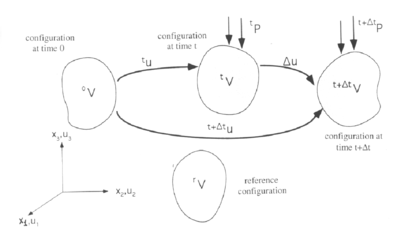
|
| Figure 1: Deformation process of a solid |
The displacements at the time are written as the sum of the known displacements and the sought displacement increments , i.e.
|
|
(1) |
Substituting the displacements in the Green strain tensor given by equation (2) and sorting the terms according to their dependence on the incremental displacements, leads to equation (3), where the strain increment vector is split into first and second order parts
|
|
(2) |
|
|
(3) |
In above and contain terms with linear and quadratic dependence on the incremental displacements , respectively, i.e.
|
A comma in a lower right index denotes a derivative with respect to the Cartesian coordinate referred to by the index following ( with ). A similar expression can be deduced for the virtual displacements. Taking into account the fact that leads to the following expressions:
|
The first and second order virtual strain increments are
|
The Piola-Kirchoff stress vector at is obtained incrementally by
|
|
(10) |
The constitutive equation chosen assumes a linear dependence between the second Piola-Kirchhoff stress increments and the Green-Lagrange strain increments as
|
|
(11) |
where is a fourth order constitutive tensor.
The expression of the PVW at time can be written as
|
|
(12) |
where are the second Piola–Kirchhoff stress and , denote the volume and surface forces, respectively. As usual and denote the volume and the boundary of the reference configuration.
Inserting equations (3) and (11) into (12) gives the full incremental form of the PVW as
|
|
(13) |
where
|
|
(14) |
Eq.(13) is the point of departure for the derivation of the secant stiffness matrix [8], [11]–[13].
As a next step the displacements and their increments are discretised in the standard finite element manner [26]
|
|
(15) |
where and are the shape function matrix and the nodal displacement vector, respectively.
The incremental secant stiffness expression is now obtained by substituting equations (4), (5), (8), (9), (10), (11) and (15) into (13) and collecting the terms depending on in the following form:
|
|
(16) |
where the incremental secant stiffness matrix is given by
|
|
(17) |
Note that the secant matrix is split in terms according to their dependence on the incremental nodal displacements . The form of the different matrices in equation (17) for truss and solid elements con be found in [8], [13] and [15] .
In eq.(16) is the residual force vector given by
|
|
(18) |
In eq.(16) is the equivalent nodal force vector deduced from eq.(14) and is the first order strain matrix relating first order strain increments and nodal displacements . The expression of this matrix can be found in [13] and [15].
Equation (16) is a non linear system of algebraic equations relating the increment of forces with the displacement increments. Indeed this secant equation can be used as a basis for deriving different non linear solution schemes to track the load–displacement pattern [13], [14]. An alternative procedure for deriving secant stiffness expressions can be found in [16].
Note that a “total” secant stiffness matrix can be obtained by making . In a total Lagrangean description (i.e. ) the total secant matrix is given by [13]
|
|
(19) |
Figure 2 shows schematically the difference between the incremental and total secant approaches. Further details can be found in [8], [13]–[15].
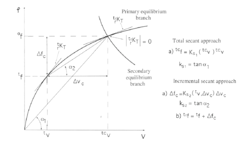
|
| Figure 2: Total (left) and incremental (right) secant approaches |
It is important to note that in the limiting case of the secant stiffness matrix reduces to the tangent stiffness matrix, i.e.
|
|
(20) |
Using the standard iteration techniques for the computation of stability points in structures can be obtained. For instance, the standard Newton–Raphson method is written from eq.(16) as
|
|
(21) |
In our work this theory was implemented for two-node truss elements and 8 node solid elements. The detailed form of all the relevant matrices can be seen in [8], [13] and [15].
2.2 Computing the equilibrium path
In order to trace the equilibrium path the load terms have to be scalable. For this purpose, the scalar load parameter is introduced. This parameter leaves the pattern of the external loads unchanged, only the size is varied (i.e. ).
The arc–length method is commonly used to calculate equilibrium solutions for different loads and displacements. Therefore the equation defining the load increment is formally extended by one equation , which determines the load parameter . A variety of different control equations can be found in the literature [4], [6]. The ones used here are stated below in equation (22).
|
|
(22) |
For the control equation the normal plane iteration was found to be rather stable and reliable in this work. Note however that the type of control equation can be problem dependent.
2.3 Prediction of instability points
The main criterion for existance of a critical point is that the tangent stiffness matrix becomes singular at the point. Mathematically this means that equation (23) below has nontrivial solutions.
|
|
(23) |
where is the critical displacement vector.
This situation corresponds to either bifurcation points, where the equilibrium path splits into a second branch, or limit points, where a snap through occurs.
The singularity of the tangent matrix has some further consequences. The determinant of is equal to in the critical point, furthermore the smallest eigenvalue is . This can be stated mathematically as
|
|
(24a) |
|
|
(24b) |
Many indirect methods for the computation of critical points use condition (24a) to determine their location on the equilibrium path. Nevertheless, in order to verify if a point indeed is a critical point these criteria can serve as test functions. Plotting , the curve should become at the critical point according to eq.(24a).
Furthermore eq.(24b) indicates that the smallest eigenvalue turns zero at . Keeping track of the number of negative diagonal elements of during the computation of equilibrium points on the path permits as well to detect critical points.
As a rather common method for critical point computation, the standard limit load analysis shall be mentioned briefly. This it is carried out by solving the following eigenvalue problem
|
|
(25) |
The estimated critical load is then obtained as a multiple of the known load at the equilibrium point.
|
|
(26) |
The approach termed as the Critical Displacement Method (CDM) [8], [14]–[16] is based on approximating the tangent matrix singularity condition at the critical point in terms of known values at the last converged solution. The unknown critical displacement field is expressed as
|
|
(27) |
where are the nodal displacements at the actual equilibrium configuration from which the prediction has to be made and is an estimate of the critical displacement increment pattern yielding structural instability at . It is now assumed to be of the form with being an approximation for the critical displacement pattern and a multiplier. As a convenient starting value of the last known value of the displacement pattern can be chosen (i.e. ).
Inserting this approximation in the expression for the tangent stiffness matrix (20) together with the condition (24a), leads to
|
|
(28) |
where the tangent matrix at the critical point has been split into terms according to their dependence on . The detailed form of the matrices involved in eq.(28) can be seen in [8] and [15]. Note that the resultant equation (28) is a quadratic eigenvalue problem, that can be solved for .
Eq.(28) can be simplified to the following standard linear eigenvalue problem by neglecting second order terms in
|
|
(29) |
For the solution of eq.(29) the Inverse Iteration method has proved to be the best [1], [4]. The Rayleigh quotient is used here as an approximation for the first eigenvalue. The convergence of this procedure can be enhanced by shifting the terms of matrix . The Jacobi iteration method as an alternative is very time consuming and thus not very suitable for large problems.
Having obtained the smallest eigenvalue , the critical displacements are predicted from equation (27) with . For the determination of the corresponding critical loads these displacements are inserted into the incremental secant stiffness matrix (see eq.(16)), which gives the prediction for the critical load as
|
The total secant stiffness matrix of eq.(19) can be used to directly calculate as shown in Figure 2. Further details can be found in [8], [13]–[15].
The approach proposed above can be applied in different ways so as to obtain the different approximations for the critical load value. For the prediction of critical points the following strategy has been used:
- A point on the equilibrium path is computed using any standard iterative procedure. As above mentioned, arc-length method based on a normal plane iteration has been chosen in this work.
- Starting from the displacements , the critical displacements are found by solving equation (29) and using eq.(27) with .
- The corresponding critical load is obtained from equations (20) and (31)
- A further point on the equilibrium path is computed
- Go to 2.
Compared to the standard limit load analysis where the critical load is obtained directly, the CDM predicts the critical displacements first. Then in an additional step the critical load is determined. Note however that the cost of the CDM is similar to that of the standard limit load computations as both involve the solution of an eigenvalue problem.
When assembling the secant stiffness matrices special care has to be taken if a damage model is included. As it will be shown next the critical displacements might belong to a damaged region in the load–deflection diagram, so that a different constitutive relation has to be applied.
3 Combination of the CDM with a damage model
In order to study the behavior of the CDM when a more complex constitutive model is used, a damage model has been implemented. Such a model permits to reproduce material failure under different stress or strain conditions. For simplicity reasons the single parameter isotropic damage model is chosen [10]. Indeed more sophisticated damage models can be used [9].
The damage parameter is a measure of the loss of secant stiffness of the material. It ranges from (undamaged material) to (fully de-gradated material). The constitutive law is now written as
|
|
(32) |
where is the damage constitutive matrix.
Similar to plasticity analysis, a damage initiation criterion and damage evolution laws have to be defined.
A damage criterion is formulated in terms of a stress norm and a damage threshold value as .
|
|
(33) |
In our work we have taken
|
In eq.(35) is the initial damage tdshreshold value and the hardening modulus. The stress norm is the square root of the product of the undamaged stress tensor with the strain tensor. For the simplest one dimensional form of this damage model, the stress–strain curve is shown in Figure 3.

|
| Figure 3: Constitutive plot for the single parameter damage model |
If inequality (33) is violated, damage occurs. The damage parameter is then updated according to the following evolution law
|
|
(36) |
which can be deduced from (35) and the damage criterion (33) when the equality sign is applied. In a damage case is no longer constant, which affects the tangent stiffness matrix . Using equations (32) and (35) the tangent constitutive matrix is obtained as
|
|
(37) |
The damage model is described in an algorithmic form.
|
Note that initially the trial stresses are computed and then compared with the actual threshold value . Following this comparison the values and are updated (damage, if–case) or not (undamaged, else–case). Index indicates here the different load levels.
4 Prediction of instability points with the CDM and a damage model
Having computed an equilibrium point with this algorithm a prediction of the critical load is made with the CDM as described in a previous section. When the approximate tangent stiffness matrix is assembled the damaged constitutive tangent matrix in order to solve equation (29). Index is used here to emphasize that the damage parameter of the current time load step corresponding to the last convergent solution in the equilibrium path is chosen. Solution of eq.(29) gives the critical displacemente pattern as previously explained.
As a next step the critical load is obtained from eqs.(30) and (31) For this purpose the incremental secant stiffness matrix has to be constructed. It is desirable to perform this computation taking into account that at the critical point elements might be in a further damaged state. The solution to this problem lies in the use of a critical damage parameter . Calculating first the critical Green stresses , the stress norm is obtained as
|
|
(38) |
The critical damage parameter is now chosen according to the following scheme:
|
|
(39) |
The option means that the damage level of the last equilibrium position is applied. Alternatively a new damage parameter is computed using the stress norm from eq.(38). The value of is then used to estimate the secant stiffness matrix at the critical point. As the critical point prediction is independent from the computation of equilibrium points on the load–deflection path, by no means an update of the damage parameter or the threshold value should be made at this prediction step.
5 Examples
In this section examples of critical point predictions using the CDM and the damage model previously described will be presented. The first two examples use two-node truss elements and the last two ones eight-node solid elements to illustrate the potential of the method.
5.1 Simple arc structure with bar elements
An outline of the first example is shown in Figure 4. The product of Young's modulus with the cross area of the bar is . A unit load is applied at the top node. All the displacements plotted in Figures 5-8 are the vertical displacements of node four. The values are multiplied by

|
| Figure 4: Discretization of the arc structure into tow node bar element |
Figure 5 shows the equilibrium path giving a limit load and a bifurcation load of . This path has been obtained by a standard incremental load process using a normal plane iteration control procedure. The detailed results correspond to values of the critical displacement and the critical load predicted from different points of the equilibrium path using the CDM with a standard (undamaged) linear elastic constitutive model. Note that a value of ( error) is predicted from the undeformed configuration.
Figures 6–8 show that introducing the damage model of previous section diminishes the value of the critical load of the structure while the values of the critical displacement are not so different. For a better comparison of results, the undamaged equilibrium path is drawn as a dotted line.
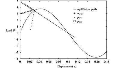
|
| Figure 5: Arc structure. Equilibrium path and critical load prediction for nondamaged material |
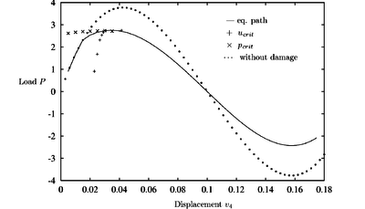
|
| Figure 6: Arc with damage: , |
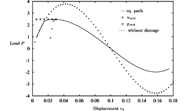
|
| Figure 7: Arc with damage: , |
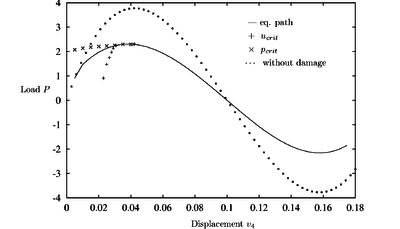
|
| Figure 8: Arc with damage: , |
The plots for different damage threshold values and hardening modulus demonstrate that the prediction follows well the new equilibrium path. The critical point predicted by the CDM is now the maximum load point. It is quite remarkable that the values of the critical load are predicted very accurately from the undeformed configurations in all cases. This is very useful for practical purposes as ideally a single computation from the original configuration should provide a good estimate of the instability load.
5.2 Curved bridge
The next example is a curved bridge formed by 35 bar elements connecting 19 nodes. (Figure 9) The arrow at node ten symbolizes again a unit load. A value of is used. In all figures the vertical displacements of node ten multiplied by versus the applied load are plotted.

|
| Figure 9: Schematic picture of the bridge |
Figure 10 shows that the CDM detects a critical point at a load level of . This bifurcation point is very close to the maximum (limit) load point .
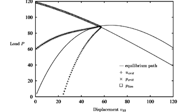
|
| Figure 10: Curved bridge. Equilibrium path and critical load prediction for nondamaged material |
Introducing damage (see Figure 11) the critical point is shifted to a lower load value of . becomes negative at a load level of and again positive at ). The CDM prediction path converges to an intermediate value between these two points. The initial critical load prediction from the the undeformed configuration is which is deviated from the actual critical load value. Progressing on the equilibrium path the predictions of the critical load and the critical displacement become more exact.
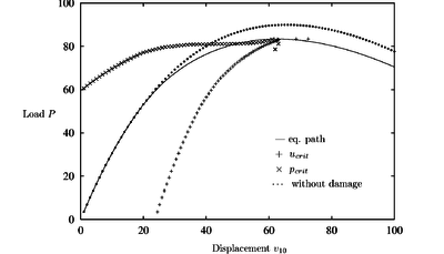
|
| Figure 11: Curved bridge with damage: , |
5.3 Shallow circular arc
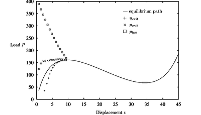
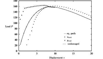
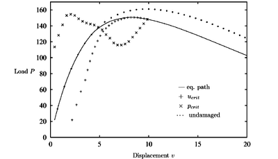
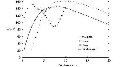
The shallow arc of Figure 12 has been studied with 2D solid elements. For symmetry reasons only one half of the arc was discretised using 10 eigth node solid elements and 53 nodes. A point load acts vertically in the middle of the arc. Both ends of the arc are clamped. The diagrams of Figures Figures 13–16) show a plot of the negative vertical displacement of the upper node in the apex of the arc versus the applied load.

|
| Figure 12: Geometry of the arc structure |
The equilibrium path in Figure 13 shows a limit point at a load level of . After the two first predictions the CDM approximates this value almost exactly.
A characteristic phenomena of all the diagrams with damage (Figures 14 - 16) is that the critical point is situated on the declining path after the maximum load has been reached. The value of the current stiffness parameter in these points indicates a critical point corresponding to a singularity of the tangent stiffness matrix.
|
| Figure 13: Shallow circular arc. Equilibrium path and critical load prediction for non damaged material |
|
| Figure 14: Shallow circular arc with damage: , |
|
| Figure 15: Shallow circular arc with damage: , |
|
| Figure 16: Shallow circular arc with damage: , |
The CDM results confirm the critical points identified by standard limit point procedures. A comparison with the undamaged predictions demonstrate the influence of the damage model in the CDM in the early states of the equilibrium path.
5.4 Hollow arc
The last example is a hollow arc with a radius of and a span of , analyzed using 10 eight node solid elements. The exact geometrical and material data can be seen in Figure 17. A vertical load is placed in the apex of the arc.

|
| Figure 17: Geometry of the hollow arc |
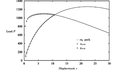
In the diagrams the vertical displacements of the lower apex node versus the applied load is plotted. Figure 18 shows results for the non damaged model. A bifurcation point is found at a load level of and a limit load point at . The first one is predicted quite accurately by the CDM even for the initial undeformed configuration ( error).

|
| Figure 18: Hollow arc. Equilibrium path and critical load predictions for non damaged material |
|
| Figure 19: Hollow arc. Equilibrium path and critical load predictions for non damaged material |
|
| Figure 20: Hollow arc with damage: , |
|
| Figure 21: Hollow arc with damage: , |
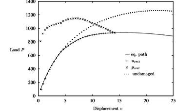
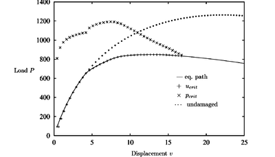
Results accounting for the effect of damage (Figures 19 and 20) show that the critical point again lies on the declining path after the maximum load. The behavior of the structure has changed and the limit and bifurcation points are closer together now. The critical load path shows a deviation when damage occurs. Note again that the CDM yielded the correct critical load value in all cases studied.
6 Conclusions
In this paper the extension of the Critical Displacement Method with a damage constitutive model for structural instability analysis using truss and solid elements was presented.
The results using the CDM were quite good for the undamaged and damaged material models and the critical point was always encountered with high precision. The values of the critical load predicted from the undeformed configuration at the cost of a single eignvalue analysis were quite accurate in most problems, with deviation in the worst case. This value can be a useful first estimate of the instability load for practical purposes.
7 Acknowledgment
The authors acknowledge the help of Dr. W.T. Matias in providing advice and the initial code for implementation of the damage model in the CDM.
REFERENCES
[1] Bathe, K. J.: Finite element procedures, Prentice Hall, Englewood Cliffs, New Jersey, 1996 [2] Bertsekas, D. P.: Constrained optimisation and Lagrange multiplier methods, Academic Press, 1982 [3] Choong, K. K., Hangai, Y.: “Review on methods of bifurcation analysis for geometrically nonlinear structures”, Bulletin of IASS, Vol. 34, no. 112, p. 133-149 [4] Crisfield, M. A.: Non–linear finite element analysis of solids and structures, Vol1, John Wiley & Sons, 1991 [5] Dawe, D.J.: “Finite deflection analysis of shallow arches by discrete element method”, International Journal of Numerical Methods in Engineering, Vol. 3 (1971) [6] Kleiber, M.: Incremental Finite Element modeling in non-linear mechanics of solids and structures, Ellis Horwood Limited, Chichester [7] Lueneberger, D. G.: Linear and nonlinear programming, Addison–Wesley, Massachusetts, 1984 [8] Matias, W.T.: The critical displacement method for structural instability analysis (in Spanish), PhD Thesis, Universitat Politecnica de Catalunya, 1996 [9] Oñate, E.: “Reliability analysis of concrete structures and numerical experimental studies”, Research Report no. 107, CIMNE, Barcelona, 1997 [10] Oliver, J., Cervera, M., Oller, S., Lubliner, J.: “Isotropic damage models and smeared crack analysis of concrete”, Second International Conference on Computer Aided Analysis and Design of Concrete Structures, Zell am See (Austria), 1990, Vol. 2, p.945-958 [11] Oñate, E., Oliver, J., Miquel, J., Suárez, B.: “A finite element formulation for geometrically nonlinear problems using a secant matrix”, Proceedings of International Conference on Computational Mechanics, Tokyo May 25-29, Springer Verlag (1986) [12] Oñate, E.: “Possibilities of the secant stiffness matrix of non linear finite element analysis”, Non Linear Engineering Computations, N. Bicanic et al. (Ed.), Pineridge Press, 1991 [13] Oñate, E.: “On the derivation and possibilities of the secant stiffness matrix for non linear finite element analysis”, Computational Mechanics, Vol.15, p. 572-593, 1995 [14] Oñate, E., Matias, W. T.: “Enhanced prediction of structural instability points using a critical displacement method”, Advances in finite element technology, N.–E. Wiberg (Eds.), CIMNE, Barcelona, 1995 [15] Oñate, E., Matias, W. T.: “A critical displacement approach for predicting structural instability”, Computer Methods in Applied Mechanics and Engineering, 134 (1996), p. 135-161 [16] Moran, A., Oñate, E. and Miquel, J., “A general procedure for deriving symmetric expressions for the secant and tangent stiffness matrices in finite element analysis”, International Journal for Numerical Methods in Engineering, Vol. 42 , pp. 219–236, 1998 [17] Riks, E.: “An incremental approach to the solution of snapping and buckling problems”, in International Journal of Solids and Structures, Vol. 15 (1979), p. 529-551 [18] Riks, E.: “Some computational aspects of the stability analysis of nonlinear structures”, in Computer Methods in Applied Mechanics and EngineeringVol. 47 (1984), p. 219-259 [19] Riks, E.: “Bifurcation and stability, a numerical approach”, in Proceedings on Innovaive Methods for Nonlinear Problems, Eds. Liu, Belytschko and Park, Pineridge Presss, p. 313-344, 1984 [20] Seydel, R.: “Numerical computation of branch points in nonlinear structural analysis”, Num. Math., Vol. 33 (1979), p. 339-352 [21] Skeie, G., Felippa, C.A.: “Detecting and traversing bifurcation points in nonlinear structural analysis”, International Journal of Space Structures, Vol. 6 (1991), p. 77-98 [22] Waszczysztn, Z.: “Numerical problems of nonlinear stability analysis of elastic structures”, Computers and Structures, Vol. 17 (1983), p. 13-24 [23] Wagner, W.: Zur Behandlung von Stabilitätsproblemen der Elastostatik mit der Methode der Finiten Elemente, Habilitation Thesis, IBNM Universität Hannover, 1990 [24] Wriggers, P., Wagner, W., Miehe, C.: “A quadratically convergent procedure for the calculation of stability points in finite element analysis”, Computer Methods in Applied Mechanics and Engineering, 70 (1988), p. 329-347 [25] Wriggers, P., Simo, J.C.: “A general procedure for the direct computation of turning and bifurcation points”, International Journal for Numerical Methods in Engineering, Vol. 30 (1990), p. 155-176[26] Zienkiewicz, O. C., Taylor: The Finite Element Method,Vol. I (1989) and Vol. II (1991), McGraw–Hill
Document information
Published on 01/01/2001
DOI: 10.1108/02644400110387190
Licence: CC BY-NC-SA license
Share this document
Keywords
claim authorship
Are you one of the authors of this document?